Exploring the Spatial Pattern and Influencing Factors of Land Carrying Capacity in Wuhan


1
School of Remote Sensing and Information Engineering, Wuhan University, Wuhan 430079, China
2
Monitoring of Wuhan Geographical Conditions group in Wuhan Geomatics Institute, Wuhan 430079, China
3
School of Public Health, University of Maryland, College Park, MD 20742-2611, USA
*
Author to whom correspondence should be addressed.
Sustainability 2019, 11(10), 2786; https://doi.org/10.3390/su11102786
Submission received: 8 April 2019
/
Revised: 5 May 2019
/
Accepted: 8 May 2019
/
Published: 15 May 2019
(This article belongs to the Special Issue Spatial Analysis and Geographic Information Systems)
Abstract
:Land carrying capacity is an important factor for urban sustainable development. It provides essential insights into land resource allocation and management. In this article, we propose a framework to evaluate land carrying capacity with multiple data sources from the first geographical census and socioeconomic statistics. In particular, an index, Land Resource Pressure (LRP), is proposed to evaluate the land carrying capacity, and a case study was carried out in Wuhan. The LRP of Wuhan was calculated on 250 m * 250 m grids, and showed a circularly declining pattern from central to outer areas. We collected its influencing factors in terms of nature resources, economy, transportation and urban construction, and then analyzed its causes via geographically weighted (GW) models. Firstly, pair-wise correlations between LRP and each influencing factor were explored via the GW correlation coefficients. These local estimates provide an important precursor for the following quantitative analysis via the GW regression (GWR) technique. The GWR coefficient estimates interpret the influences on LRP in a localized view. Results show that per capita gross domestic product (PerGDP) showed a higher absolute estimate among all factors, which proves that PerGDP has a relieving effect on LRP, especially in the southwestern areas. Overall, this study provides a technical framework to evaluate land carrying capacity with multi-source data sets and explore its localized influences via GW models, which could provide practical guidance for similar studies in other cities.
1. Introduction
Rapid industrialization and urbanization in China have led to various contradictions particularly between increasing demands for socio-economic development and critical resource reserves [1,2,3]. Therefore, excessive resource consumption and environmental sacrifice have been frequently studied [4,5,6]. In particular, land utilization and carrying capacity have always been crucial components of urban sustainable development [7,8]. Studies on urban land carrying capacity can involve carriers (including residential land, industrial land and transportation land), objects (i.e., population and industry), and influencing factors (including locational properties, geological conditions, human production and living demands) [9,10].
Land carrying capacity is traditionally defined to explore relationships between land resources and its maximum population capacity [11]. It is usually used in cities as a research object on a really coarse scale [12,13]. Attempts to evaluate land carrying capacity at finer scales have yet to be made. The first national geographic census in China started in 2013 and provides an ideal data support for this purpose. During this activity, natural objects and man-made objects were widely collected with high-resolution remote sensing images and related surveying products, including digital orthophoto map (DOM), digital elevation model (DEM), digital line graphic (DLG) and digital raster graphic (DRG) [14,15]. These data products are characterized by high accuracy and abundant information. For example, land cover classification data (LCA) contain ten top categories and more than 100 sub-categories [16]; the house building data include not only shape and location but also the number of floors. These products provide essential data sources for evaluating land carrying capacity.
From the perspective of development and utilization, a number of methods have been proposed to evaluate land carrying capacity. Land-use intensity and population aggregation are the most important components of land carrying capacity. The influencing factors have been studied variously, with natural resources including vegetation [17], water [18], economy including gross domestic product (GDP) [19], urban economic structure [20], and transportation [21,22].
To analyse the local influences of those factors on land carrying capacity, we introduce geographically weighted (GW) techniques, including GW summary statistics and GW regression (GWR) [23,24]. In this study, we preliminarily explored pair-wise GW correlation coefficients between LRP and its influence variables, and we then applied the GWR technique to explore the localized relationships between it and multiple exploratory variables in order to better understand it [25]. The results reflect the heterogeneous characteristics of the land carrying capacity in Wuhan, and are helpful for the sustainable use of land resources.
2. Data and Methodologies
2.1. Study Area
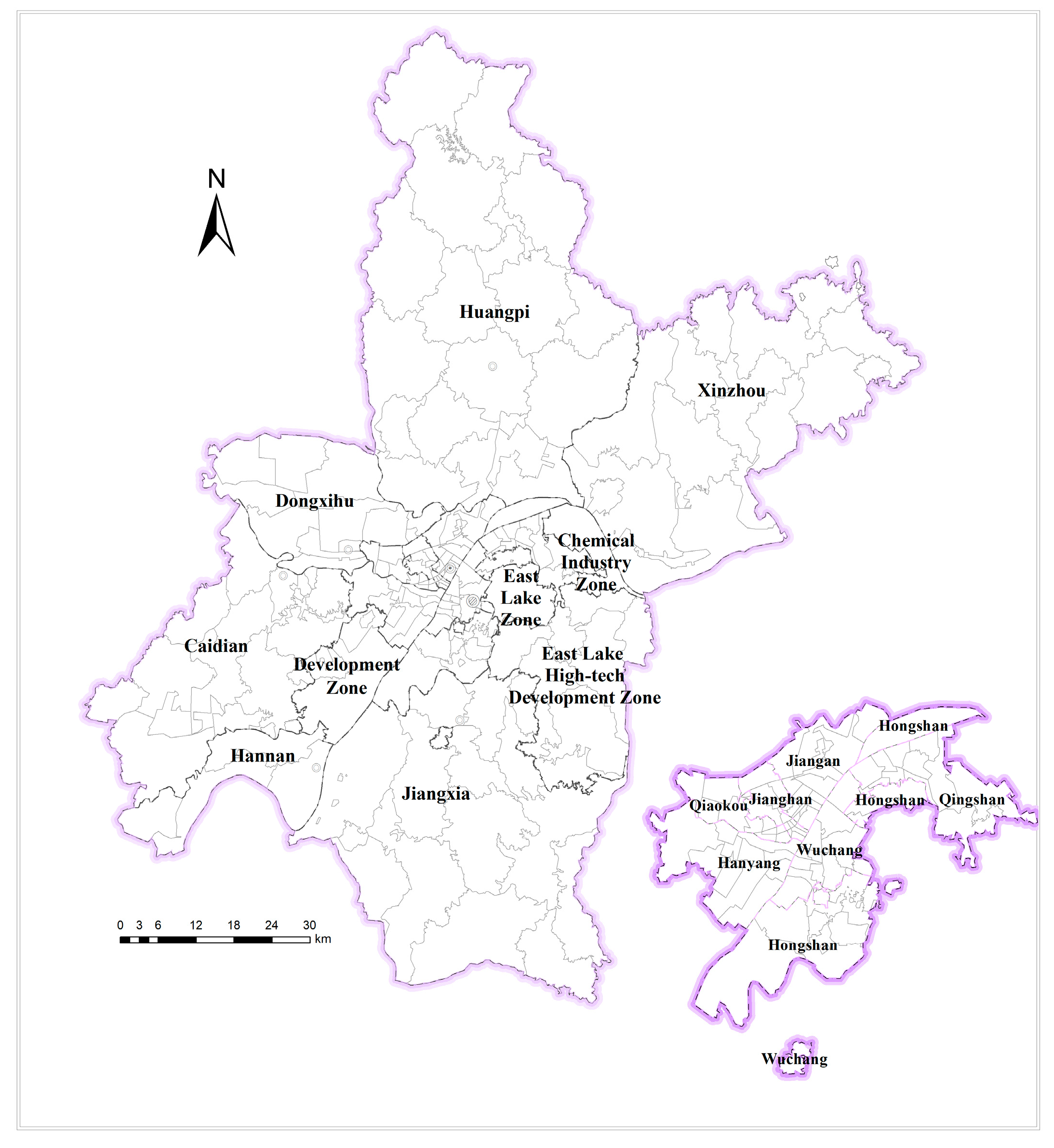
As one of the most important cities in central China, Wuhan acts as an important base for industry, science, education and transportation hubs [26]. There are four levels of administrative divisions in Wuhan: city, municipal districts, townships and communities. It is composed of 13 municipal districts and three state-level development zones, with a total area of 8494.41 km2. Its population is 10,766,200 in 2016, and the urbanization rate is 79.77% [27]. Figure 1 shows the location of Wuhan. It consists primarily of undulating landforms alternating between hills and plains, with mountains in the north and water in the south. With an area of 1862.43 km2, Wuhan is rich in water, ranking top of 334 cities in China. Due to its natural conditions, the development and utilization of Wuhan started and clustered in the central plain areas.
2.2. Data Geo-Processing and Influencing Factors
2.2.1. Data Geo-Processing
Data collected for this study contains two main parts. (i) One is the spatial datasets from the first geographical census in 2016, including DEM, digital terrain model (DTM), LCA, urban road network, and bus lines. (ii) The other part includes annual statistics on the economy of the district level and demographic data of the community level. To facilitate the multi-source data fusion, spatialization was performed for the latter part of the data sets. We associated the annual statistics with the corresponding administrative districts by name. In particular, GDP data was divided into three parts from the primary, secondary and tertiary industries, as shown in Table 1.
For a finer-scaling spatial analysis, it was necessary to construct a grid based on demographic data. Li et al. [28] indicated that the 250 m * 250 m population grid shows a higher accuracy with the same datasets from the National Earth System Science Data Sharing Infrastructure (http://www.geodata.cn). Therefore, we also used a 250 m * 250 m fishnet of Wuhan City in this study. The theoretical number of people per building could be calculated on the base of the number of dwellings and the average population of each dwelling [29]. Accordingly, the theoretical number of people per grid could be calculated with the residential areas and the average population density.
2.2.2. Influencing Factors
In this study, ten influencing factors were collected in terms of nature resources, economy, transportation and urban construction, as interpreted in Table 2. These variables cover the key concerns of government management in terms of LRP, which are important for decision-making. They could be extracted from the collected datasets. Particularly, the yearly updating strategy of these datasets would provide strong support for the subsequent studies on LRP. In particular, the spatial datasets are provided annually by the Monitoring of Wuhan Geographical Conditions group, and the socioeconomic statistics are published yearly by Wuhan Bureau of Statistics.
Variables grouped in nature resources describe the natural conditions of each grid, including the ratio of vegetation (Vegetation) and the ratio of water (Water). The two variables were extracted from the LCA data. In detail, Vegetation includes land covers of woodland and grassland, and Water refers to rivers, lakes and ponds. Variables of the economy group include the added values of primary industry (PrimaryIndustry), secondary industry (SecondaryIndustry) and tertiary industry (TertiaryIndustry). We also calculated the per capita gross domestic product (PerGDP) of each township. In addition, transportation was considered as another important affecting factor on land development [30]. Variables of this group include road network density (RoadDensity), bus line density (BusDensity) and ratio of the 500 m subway buffer (SubCover) within each township. Finally, the proportion of urban construction lands (Construction), like commercial services and public facilities, were also prepared at grid level. Note that all these variables could be sampled on different units, grids or administrative hierarchies. The multi-level data structures might potentially affect the results of local models due to their distinctive features in spatial dependence [31], which forms an interesting topic to be studied further.
2.3. Land Resource Pressure Index
In this study, we proposed a land resource pressure index (LRP) to evaluate the current status of land carrying capacity. It was calculated with both land development degree and population. Land development usually promotes population agglomeration. Meanwhile, population concentration implies intensive resource consumption [32]. Land development and population are indivisible and work jointly on land carrying capacity. The status of land development degree reflects the current utilization level of land resources. In this study, the land development degree of each grid was evaluated by considering both land used and land suitable for construction. We computed the ratios of the population density of each grid and the average population density of Wuhan city, and used them as population factors.
Firstly, the suitable land for construction can be calculated via the following formula:
where represents the suitable land for construction, means slope, means elevation, and represents areas unsuitable to be developed. The ‘’, ‘-’ and ‘’ symbols in Equation (1) represent the intersection, subtraction and union geoprocessing operations, respectively.
With an increasing slope, land becomes more difficult for construction, and could be more prone to geological disasters. We reclassified and weighted the and classes. After subtracting , we chose areas with scores above 80 as suitable land for construction. The adapted criteria is presented in Table 3 [33,34].
A small piece of land cover merged into its surrounding larger areas in the data production process of the first geographical census, for example, ridges with area less than 400 m2 would be merged with the cultivated field. Meanwhile, the combination with the population grid was important for calculating LRP. This is the other reason why we choose a 250 m * 250 m grid for this study. The Modifiable Areal Unit Problem (MAUP) is worth noting [35]; aggregation scales may bring about different messages, but the distributions of the results should have some commonality.
The land development degree for each grid can be expressed as follows:
where is the development degree of the land in the ith grid, and represents used land for construction.
The population factor is standardized as follows:
where is the population density of each grid, and is the average population density of Wuhan city. Note that we normalized the to a range of 0.00–1.00.
Finally, we can calculate the LRP index via the following formula:
2.4. Geographically Weighted Models
In this study, we used GW models, including GW summary statistics and GWR to explore the localized relationships between LRP and its influence factors, including natural resources, economy, and transportation. Specifically, relative functions in the R package GWmodel were used here.
2.4.1. GW Summary Statistics
GW summary statistics provide local views in exploratory spatial data analysis and can be an important precursor for the following GWR analysis. In detail, GW summary statistics include GW mean (Equation (5)), GW standard deviation (Equation (6)), GW covariance (Equation (7)), and GW correlation coefficient (Equation (8)). They can be expressed as follows:
where represents the spatial coordinate at location i, and refer to attributes, and is the weight calculated via a kernel function. A kernel function is defined as a decreasing function of distance with values ranging from 0.00 to 1.00 [36]. In this study, we selected the Bi-square function to calculate .
2.4.2. Geographically Weighted Regression
A GWR model can be generally expressed as follows:
where is the dependent variable at location , is the value of the kth independent variable, m is the number of the independent variables, is the intercept parameter at location i, is the local regression coefficient of the kth independent variable at location i, and is random error.
GWR makes location-wise calibrations via the weighted least squares method, and its matrix expression is as follows:
where X is the matrix of the independent variables with the fist column of 1s for the intercept, y is the dependent variable vector, is a vector of m + 1 local regression coefficients, and is an diagonal matrix denoting the geographical weighting of each observed data for location i. In particular, we chose Gaussian kernel function via several attempts and optimized an adaptive bandwidth via the corrected Akaike information criterion (AICC) approach.
3. Results and Discussion
3.1. Spatial Pattern of the Land Resource Pressure
In total, there are 3774.42 km2 of land suitable for construction, and 1484.12 km2 has been developed up until 2016. Figure 2a,b map the suitable land, used and unused land of Wuhan. In the Huangpi and Xinzhou districts, there is 319.34 km2 of suitable land, i.e., 33.10%, but higher suitability scores appear in southwestern areas, like the Hannan district with a score up to 100.
Figure 3 presents the population and development degree map of Wuhan in 250 m * 250 m grids. The population apparently clusters in the central area along the Yangtze River and the Han River, while it shows a decreasing trend from the central part to the outer areas. In Figure 3b, we also present the grid-level development degree (DL) within Wuhan. It could be expected that the central areas are highly developed, which is confirmed by the population distributions as shown in Figure 3a.
With the data processed, we calculated the LRP index for each grid via the method proposed in Section 2.3, of which the map is shown in Figure 4a. It shows a very similar distribution as to the population (Figure 3a), which indicates that population could be the most important driving force of the LRP. The highest pressure appears in the Jianghan district (Figure A1 maps the districts in Wuhan), where the LRP index reaches 1, and its population density is 61.97 times higher than the average density of Wuhan. The lowest pressure appears in the Tianxing community of the Hongshan district, where the LRP index is only 0.10, and its population density is only 1/20 of the average density of Wuhan.
In view of its typically circular pattern, we also plotted LRP versus the distance from the geometric center of Wuhan city to each township (Figure 4b). Figure 4b shows that extremely high values of LRP appear in townships within 15 km from the city center, while much lower values distribute in the outer areas. Red, green and blue colors represent three different categories of administrative districts, respectively: central, functional and new urban districts. Townships located in central urban districts have the smallest average area but the highest LRP, while the difference of LRP between functional districts and new urban districts is not significant.
3.2. GW Correlation Coefficients
The LRP index is closely related to land development and population agglomeration. Specifically, areas of gentle topography tend to be developed in the first place due to low cost of construction, for residence, transportation or industry. People settle in these areas, which results in high pressures on land resources. In this section, we explore the relationships between the LRP index and its influencing factors with regard to natural resources, economy, transportation and urban construction via GW correlation coefficients with the GWmodel package. We present the summarized GW correlation coefficients in Table 4, and their density plots in Figure 5. Results show that most of the influencing factors are highly related to LRP.
In terms of natural resources, most values are negative, suggesting that vegetation and water make development more difficult. For Vegetation, the GW correlation coefficients are relatively even with both negative and positive values, while negative correlations appear more. LRP and Water present negative correlations in most places, where 80% of the GW correlation coefficients are negative.
For economic factors, pair-wise correlated relationships between industrial categories and LRP are explored. The PrimaryIndustry index shows negative correlations with LRP in most areas, which indicates that the rural areas in Wuhan have great potential for future development. In contrast, both SecondaryIndustry and TertiaryIndustry present positive GW correlation coefficients with LRP in most places, and tertiary industries particularly show much stronger effects on LRP. These results are in line with Wuhan playing a role as one of the core cities within central China during rapid urbanization. Surprisingly, the GW correlation coefficients between PerGDP and LRP are negative in most areas, which demonstrates that the industrial level is not dependent on the production factors. The advancement of science and technology reduces the demand for land in the economy.
From the perspective of transportation factors, most GW correlation coefficients are positive, which indicates that high pressures on land resources are always accompanied by well-developed transportation facilities. Figure 5c shows that there are more positive values for RoadDensity and BusDensity, because subway merely covers the central part of Wuhan, while urban road and bus lines cover most areas with gradual expansions to the suburbs.
With respect to urban constructions, the GW correlation coefficients of Construction index present similar patterns as those of Vegetation. Negative coefficients appear more frequently. High-efficiency land use, such as Construction, might have a certain impact on reducing LRP.
3.3. GWR Results
To explore the relationships between LRP and its influence factors (as shown in Table 2) quantitatively, we used the GWR technique and compared it with the ordinary least squares (OLS) technique. Specifically, the candidate exploratory variables were counted in a 1 km grid. To avoid the multicollinearity problem, variance inflation factors (VIF) were calculated. Variables were eliminated if the VIF value is suspiciously large (for example, greater than 7.5) [37]. We used a final model with eight independent variables, including Vegetation, Water, PrimaryIndustry, TertiaryIndustry, PerGDP, RoadDensity, BusDensity and Construction. In this model, all the VIF values of independent variables did not exceed 7.5. The GWR model was then calibrated with an optimized adaptive bandwidth.
We have summarized the results in Table 5. The GWR model performs much better than the OLS model by increasing the adjusted R2 value from 0.5457 to 0.6157 and reducing the AICc value from −38,296.94 to −39,774.340. We also produced a map of the local R2 values from the GWR results in Figure 6. The higher the local R2, the better the local model performs [38,39]. High local R2 values mostly appear in the central areas, while the GWR model shows poorer fits in north and south, particularly in Huangpi and Hannan districts.
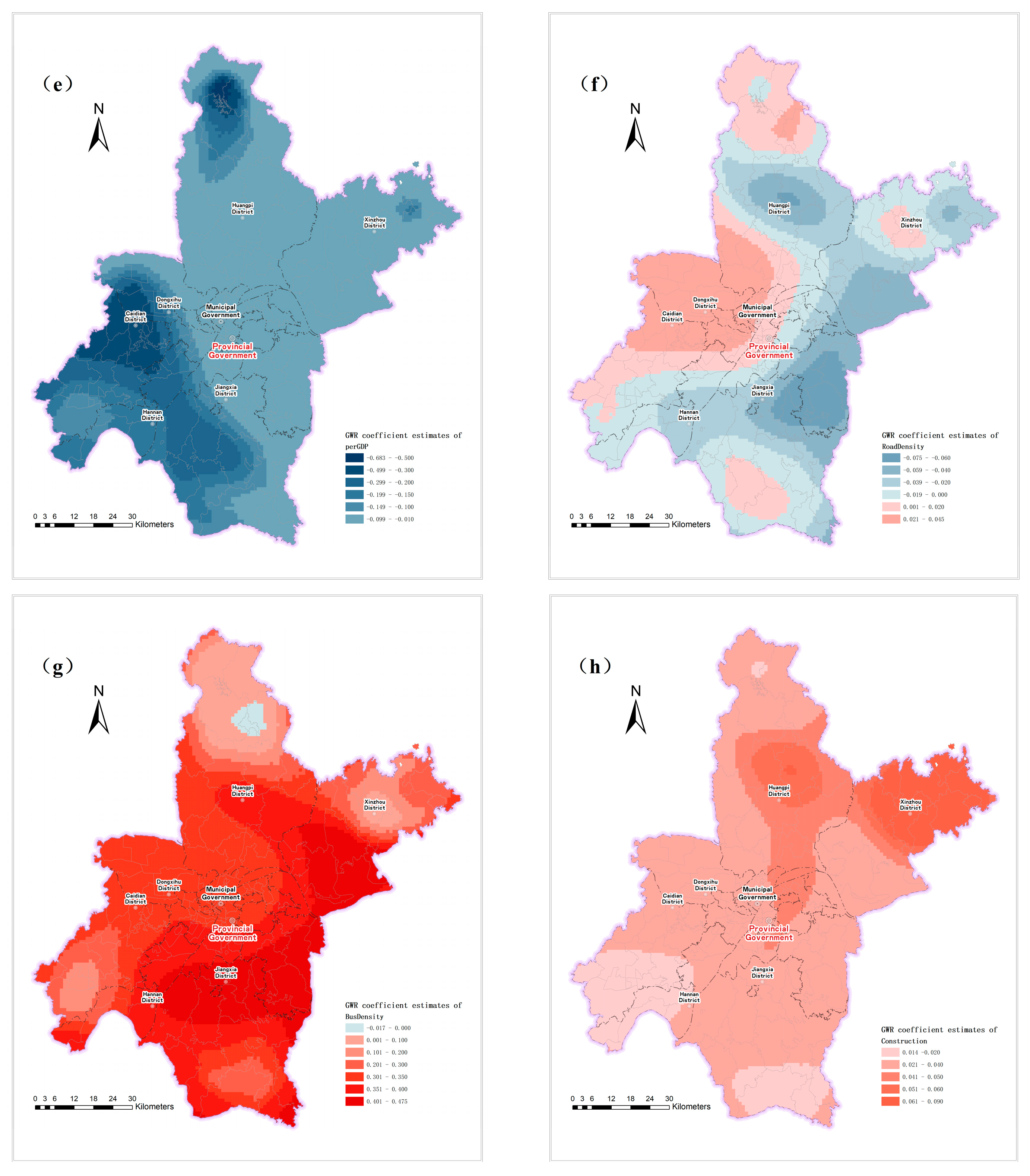
The data classification of a map affect its readability [40]. According to the distribution of the GWR coefficient estimates, constant intervals were used for manual classification with 0, including 0.02, 0.04, 0.06, 0.10, 0.15, 0.20, 0.30 and 0.50. Figure 7a–h map the GWR coefficient estimates. Red hue indicates a positive symbol, while blue hue indicates a negative symbol on LRP; greater saturation corresponds to larger absolute values of the regression coefficient. As shown in Figure 7a–h, the GWR coefficient estimates present spatially varying patterns in a quantitative view.
Natural conditions could essentially affect regional developments. In this study, Vegetation and Water were incorporated to analyze their influences on the LRP index, and negative relationships were mostly found (Figure 7a,b). In particular, strong negative coefficients are acquired in the central part, like the Jianghan, Hanyang and Hongshan districts. The negative estimates could be rationally caused by the restrictions of water bodies and reserving policies of vegetation in land development. Note that the estimates of Vegetation are of higher absolute values, which might indicate stronger impacts than those of water bodies.
Figure 7c,d map the GWR coefficient estimates of economic industrial structure. PrimaryIndustry and TertiaryIndustry show positive effects on LRP in most areas. High values of PrimaryIndustry appear in the Dongxihu and Hanyang districts, which have a large population. The more farmland there is, the less land available for living. This will result in a high population concentration within fragmenting small areas. Especially in the Xinzhou district, the coefficient estimates of TertiaryIndustry show negative values. This phenomenon could be related to the industrial structure that SecondaryIndustry is much higher than TertiaryIndustry in this area.
PerGDP is an effective indicator to reflect daily living level and social development degree. The values are negative in Figure 7e, which suggest that both the living improvement and social progress can relieve LRP. Note that the GWR estimates of PerGDP are of the highest absolute values.
The estimates of RoadDensity are presented in Figure 7f. RoadDensity mostly shows positive impacts in the western areas, where residential land accounts for a large proportion. The migrations caused by traffic development could be an oblique reason why the LRP is increased. However, the estimates are negative in the eastern areas of Wuhan. Note that production industries and enterprises gather in these areas, and transportation facilities mostly work for manufacture and construction. Figure 7g,h map the estimates of BusDensity and Construction. Positive impacts on LRP could be found for both, and high values could be found in Jiangxia, Xinzhou and the East Lake High-tech Development Zone, which indicate typical relations between land development and LRP.
4. Conclusions
In this article, we proposed an index, LRP, to evaluate the pressure of current land resources, as a status indicator of land carrying capacity with considerations of influence factors in nature resources, economy, transportation and urban construction. A case study of Wuhan city was conducted. Restricted by topographic conditions and development policies of Wuhan, construction and population mainly concentrate in the central area of Wuhan. This leads to a typically declining circular distribution of LRP.
We explored the spatially varying relationships between the LRP and its influence factors via calculating pair-wise GW correlation coefficients and the GWR technique, which provided a basis for the sustainable development of land resources. GW correlation results indicate that most of the influencing factors are highly related to LRP and provide an important precursor for the GWR calibration. The results show that GWR provides a better fit than the OLS according to their diagnostic information, and the causes of LRP could be also interpreted at a finer scale, i.e., spatially varying patterns.
The LRP and its potential causes explored in this study could provide strong support in future policy making. Note that over 60% of the total population settle in an area that is only 7% of the whole of Wuhan city (Figure 3a), and the LRP shows a typically declining circular distribution (Figure 4a). The unbalances in urban development of Wuhan, reflected by the social-economic factors, lead to a typical distribution of LRP within Wuhan. A polycentric development strategy could be preferable for the urban development of Wuhan in the future, like promoting the development of Guanggu and the East Lake High-tech Development Zone, to prompt a more balancing LRP distribution. In addition, specific policies could be made accordingly with the estimates of natural resource and transportation variables.
Furthermore, we took the first geographical census data of high spatial and attribute accuracies as the main data source in this study. The integration with socio-economic data, however, is still open to be investigated. For instance, the process of building extraction may include non-residential or demolished houses, which could impact the accuracy of population density. To solve the above mentioned problems, residential areas from building survey or point of interest (POI) data can be used in future studies. They can be helpful in removing improper types of buildings, such as shopping malls, libraries, offices, etc. The population data used here were drawn from the government census data, of which the scale is rarely coarse on our studied level. With the development of spatio-temporal big data, cellular data or social-media data can be adopted to produce finer scaled population data. The present study can be regarded as a preliminary exploration of the relationships between LRP and its influencing factors via the GW techniques. Future work can focus on more accurate methodologies by considering hierarchical data structures [31], multi-scale [41,42] or collinearity [43,44,45] issues with a considerable number of exploratory variables.
Author Contributions
Methodology, J.L. and B.L.; data curation, N.Y. and L.L.; writing—original draft, N.Y.; revising draft, B.L and M.L.
Funding
National Key Research and Development Program of China (No. 2018YFC0407804); Natural Science Foundation of China grant number [NSFC: U1833201; 41871287]; Jointly funded by the Wuhan Geomatics Institute.
Acknowledgments
The spatial data (such as LCA, the urban road, the bus line, etc.) of geographical census in 2016 were supported by the Monitoring of Wuhan Geographical Conditions group in Wuhan Geomatics Institute. We would like to thank ZiLong Jiang at the College of Urban & Environment Sciences, Central China Normal University, and YiLin Shi at the School of Remote Sensing and Information Engineering, Wuhan University for their expertise that helped us complete this research.
Conflicts of Interest
The authors declare no conflict of interest.
Appendix A
Figure A1.
Territorial division of Wuhan—districts.
References
- Jung, H.B. Nutrients and heavy metals contamination in an urban estuary of northern new jersey. Geosciences 2017, 7, 108. [Google Scholar] [CrossRef]
- Zhang, J.; Fu, M.; Zhang, Z.; Tao, J.; Fu, W. A trade-off approach of optimal land allocation between socio-economic development and ecological stability. Ecol. Model. 2014, 272, 175–187. [Google Scholar] [CrossRef]
- Shao, W.W.; Zhou, Z.H.; Liu, J.H.; Yang, G.Y.; Wang, J.H.; Xiang, C.Y.; Cao, X.L.; Liu, H.Z. Changing mechanisms of agricultural water use in the urbanization and industrialization of China. Water Policy 2017, 19, 908–935. [Google Scholar] [CrossRef]
- Cairns, R.D.; Martinet, V. An environmental-economic measure of sustainable development. Eur. Econ. Rev. 2014, 69, 4–17. [Google Scholar] [CrossRef] [Green Version]
- Rydzewski, P. The implementation of sustainable development vs. environmental attitudes in international comparative studies. Probl. Ekorozw. 2013, 8, 125–137. [Google Scholar]
- Tong, Y.Q. Bureaucracy meets the environment: Elite perceptions in six Chinese cities. China Q. 2007, 189, 100–121. [Google Scholar] [CrossRef]
- Ye, L.M.; Van Ranst, E. Population carrying capacity and sustainable agricultural use of land resources in Caoxian County. J. Sustain. Agric. 2002, 19, 75–94. [Google Scholar] [CrossRef]
- Lane, M. The carrying capacity imperative: Assessing regional carrying capacity methodologies for sustainable land-use planning. Land Use Policy 2010, 27, 1038–1045. [Google Scholar] [CrossRef] [Green Version]
- Yang, L.; Lv, Y.; Zheng, H.Y. Review on research of urban land carrying capacity. Prog. Geogr. 2010, 29, 593–600. [Google Scholar]
- Wei, Y.G.; Huang, C.; Lam, P.T.I.; Yuan, Z.Y. Sustainable urban development: A review on urban carrying capacity assessment. Habitat Int. 2015, 46, 64–71. [Google Scholar] [CrossRef]
- UNESCO; FAO. Carrying Capacity Assessment with a Pilot Study of Kenya: A Resource Accounting Methodology for Exploring National Options for Sustainable Development; UNESCO: Paris, France; FAO: Rome, Italy, 1985. [Google Scholar]
- Lin, W.; Chen, Y. The impact of urbanization on land carrying capacity in Beijing-Tianjin-Hebei region. Argo Food Ind. Hitech 2017, 28, 3747–3751. [Google Scholar]
- Yan, H.M.; Liu, F.; Liu, J.Y.; Xiao, X.M.; Qin, Y.W. Status of land use intensity in China and its impacts on land carrying capacity. J. Geogr. Sci. 2017, 27, 387–402. [Google Scholar] [CrossRef]
- Zhang, J.X.; Liu, J.P.; Zhai, L.; How, W. Implementation of geographical conditions monitoring in Beijing-Tianjin-Hebei, China. ISPRS Int. J. Geo-Inf. 2016, 5, 89. [Google Scholar] [CrossRef]
- Li, D.R.; Ding, L.; Shao, Z. Considerations on several issues concerning monitoring of geo-graphical conditions. Geomat. Inf. Sci. Wuhan Univ. 2016, 41, 144–147. [Google Scholar]
- Zhang, J.; Li, W.; Zhai, L. Understanding geographical conditions monitoring: A perspective from china. Int. J. Digit. Earth 2015, 8, 38–57. [Google Scholar] [CrossRef]
- Pozzi, F.; Small, C. Exploratory analysis of suburban land cover and population density in the USA. In Proceedings of the IEEE/ISPRS Joint Workshop on Remote Sensing and Data Fusion over Urban Areas (Cat. No.01EX482), Rome, Italy, 8–9 November 2001; pp. 250–254. [Google Scholar]
- Xu, Y.Q.; Li, Y.H.; Zhao, F.F. Simulation of land use change under the restriction of water resource in ecologically fragile region: A case study of Zhangbei County, Hebei Province. J. China Agric. Univ. 2015, 20, 214–223. [Google Scholar]
- Peng, C.; Song, M.L.; Han, F. Urban economic structure, technological externalities, and intensive land use in China. J. Clean. Prod. 2017, 152, 47–62. [Google Scholar] [CrossRef]
- Liu, N.; Shi, P.J.; Li, B. Space difference and correlation between population and economy in Gansu Province. Arid Land Geogr. 2014, 37, 179–187. [Google Scholar]
- Zhang, R.S.; Pu, L.J.; Zhu, M. Impact of transportation arteries on land use patterns in urban-rural fringe: A comparative gradient analysis of Qixia District, Nanjing City, China. Chin. Geogr. Sci. 2013, 23, 378–388. [Google Scholar] [CrossRef]
- Song, G.B.; Li, Z.H.; Bao, Y.J.; Lu, H.Y.; Gao, J.X.; Wang, H.M.; Xu, T.; Cheng, Y. Spatial distribution regularity and influence factors of population density in the LRGR. Chin. Sci. Bull. 2007, 52, 90–97. [Google Scholar] [CrossRef]
- Brunsdon, C.; Fotheringham, A.S.; Charlton, M. Geographically weighted summary statistics—A framework for localised exploratory data analysis. Computers. Environ. Urban Syst. 2002, 26, 501–524. [Google Scholar] [CrossRef]
- GolliniI, I.; Lu, B.; Charlton, M.; Brunsdon, C.; Harris, P. GWmodel: An R package for exploring spatial heterogeneity using geographically weighted models. J. Stat. Softw. 2015, 63, 1–50. [Google Scholar] [CrossRef]
- Fotheringham, A.S.; Brunsdon, C.; Charlton, M. Geographically Weighted Regression: The Analysis of Spatially Varying Relationships; Wiley: Chichester, UK, 2002. [Google Scholar]
- Han, S.S.; Wu, X.A. City profile Wuhan. Cities 2004, 21, 349–362. [Google Scholar] [CrossRef]
- Wuhan Statistics Bureau. Wuhan National Economic and Social Development Statistical Bulletin in 2016. Available online: http://www.whtj.gov.cn/details.aspx?id=3439 (accessed on 31 March 2017).
- Li, L.; Li, J.; Jiang, Z.; Zhao, L.; Zhao, P. Methods of population spatialization based on the classification information of buildings from china’s first national geoinformation survey in urban area: A case study of Wuchang district, Wuhan city, China. Sensors 2018, 18, 2558. [Google Scholar] [CrossRef] [PubMed]
- Szombara, S. Automation of Dot Maps Production Supported by BDOT10k Database. In Proceedings of the 2017 Baltic Geodetic Congress (BGC Geomatics), Gdansk, Poland, 22–25 June 2017; pp. 100–104. [Google Scholar]
- Li, S.J.; Zhou, C.S.; Wang, S.J.; Gao, S.; Liu, Z.T. Spatial Heterogeneity in the Determinants of Urban Form: An Analysis of Chinese Cities with a GWR Approach. Sustainability 2019, 11, 479. [Google Scholar] [CrossRef]
- Dong, G.P.; Richard, H. Spatial Autoregressive Models for Geographically Hierarchical Data Structures. Geogr. Anal. 2015, 47, 173–191. [Google Scholar] [CrossRef]
- Schneider, A.; Mertes, C.M. Expansion and growth in Chinese cities, 1978–2010. Environ. Res. Lett. 2014, 9, 024008. [Google Scholar] [CrossRef] [Green Version]
- Xu, Y.; Tang, Q.; Fan, J. Available land index items and their calculational methods for major function oriented regionalization. Geogr. Res. 2010, 29, 1223–1232. [Google Scholar]
- Xu, X.R.; Xu, Y. Potential of available construction land in the Yangtze River economic belt. Resour. Environ. Yangtze Basin 2016, 25, 1789–1795. [Google Scholar]
- Openshaw, S. The Modifiable Areal Unit Problem; Geo Books: Norwich, UK, 1984; p. 3. [Google Scholar]
- Lu, B.; Charltion, M.; Harris, P.; Fotheringham, A.S. Geographically weighted regression with a non-euclidean distance metric: A case study using hedonic house price data. Int. J. Geogr. Inf. Sci. 2014, 28, 660–681. [Google Scholar] [CrossRef]
- Pak, M.; Gulci, S.; Okumus, A. A study on the use and modeling of geographical information system for combating forest crimes: An assessment of crimes in the eastern Mediterranean forests. Environ. Monit. Assess. 2018, 190, 62. [Google Scholar] [CrossRef] [PubMed]
- Lewandowska-Gwarda, K. Geographically Weighted Regression in the Analysis of Unemployment in Poland. ISPRS Int. J. Geo-Inf 2018, 7, 17. [Google Scholar] [CrossRef]
- Török, I. Qualitative Assessment of Social Vulnerability to Flood Hazards in Romania. Sustainability 2018, 10, 3780. [Google Scholar] [CrossRef]
- Całka, B. Comparing continuity and compactness of choropleth map classes. Geod. Cartogr. 2018, 67, 21–34. [Google Scholar]
- Lu, B.; Brunsdon, C.; Charlton, M.; Harris, P. Geographically weighted regression with parameter-specific distance metrics. Int. J. Geogr. Inf. Sci. 2017, 31, 982–998. [Google Scholar] [CrossRef]
- Fotheringham, A.S.; Yang, W.; Kang, W. Multiscale Geographically Weighted Regression (MGWR). Ann. Am. Assoc. Geogr. 2017, 107, 1247–1265. [Google Scholar] [CrossRef]
- Brunsdon, C.; Charlton, M.; Harris, P. Living with collinearity in Local Regression Models. In Proceedings of the Accuracy 2012—10th International Symposium on Spatial Accuracy Assessment in Natural Resources and Environmental Sciences, Florianópolis, Brazil, 10–13 July 2012. [Google Scholar]
- Fotheringham, A.S.; Oshan, T.M. Geographically weighted regression and multicollinearity: Dispelling the myth. J. Geogr. Syst. 2016, 18, 303–329. [Google Scholar] [CrossRef]
- Comber, A.; Chi, K.; Huy, M.Q.; Nguyen, Q.; Lu, B.; Phe, H.H.; Harris, P. Distance metric choice can both reduce and induce collinearity in geographically weighted regression. Environ. Plan. B Urban Anal. City Sci. 2018. [Google Scholar] [CrossRef]
Figure 1.
Map of Wuhan.


Figure 2.
Map of (a) suitable land (E), (b) used land (S) and unused but suitable land in Wuhan.

Figure 3.
Map of (a) resident population, (b) development degree (DL) (250 m * 250 m grid) in Wuhan. Note: we zoom in on the top right to show the result for the central area.
Figure 3.
Map of (a) resident population, (b) development degree (DL) (250 m * 250 m grid) in Wuhan. Note: we zoom in on the top right to show the result for the central area.
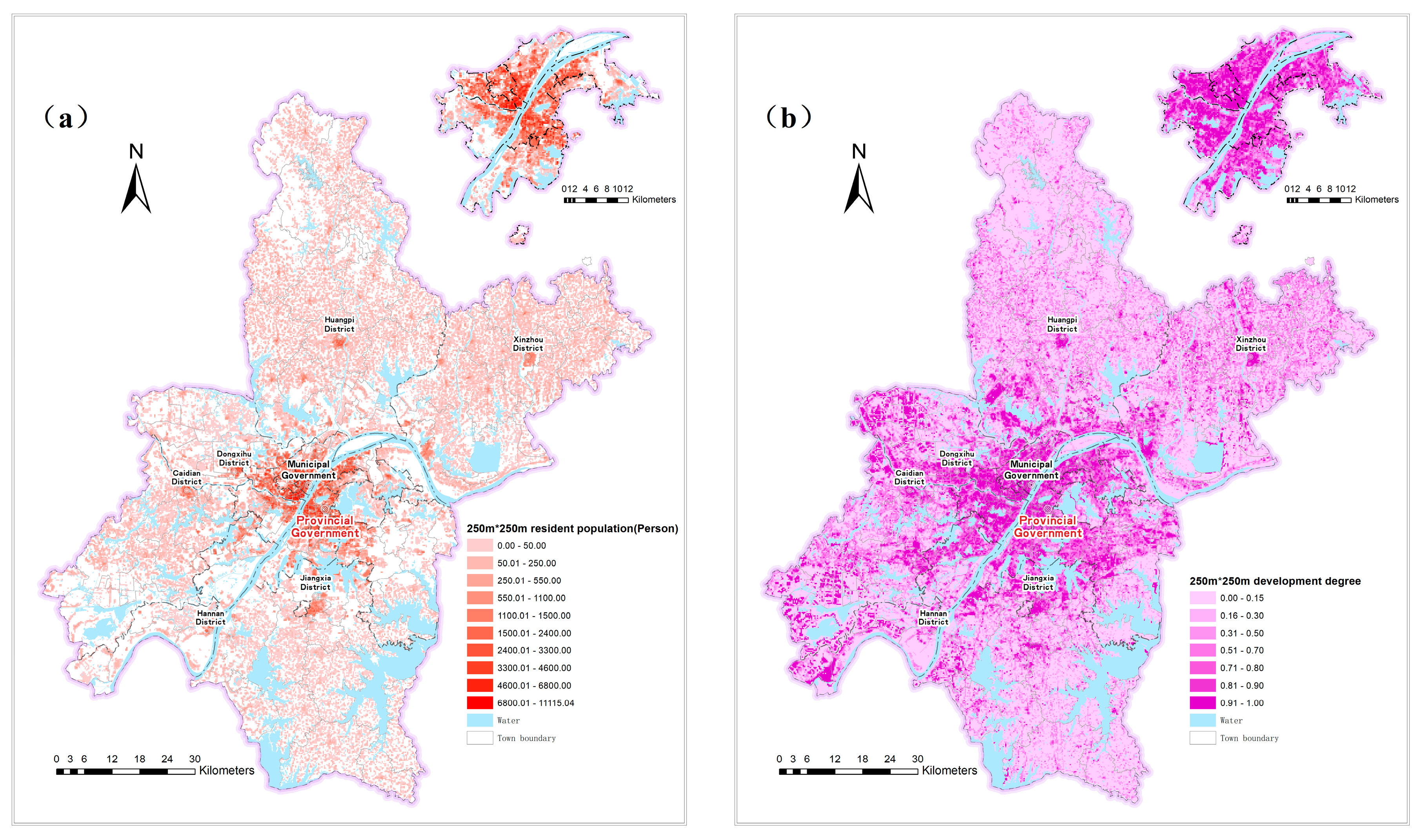
Figure 4.
(a) LRP, (b) scatter plot of LRP between the distances of each township from the city center. Note: we zoom in on the top right of Figure 4a to show the result for the central area.
Figure 4.
(a) LRP, (b) scatter plot of LRP between the distances of each township from the city center. Note: we zoom in on the top right of Figure 4a to show the result for the central area.

Figure 5.
Density of GW correlation coefficients between LRP and its influence factors in (a) natural resources; (b) economy; (c) transportation; (d) urban construction.
Figure 5.
Density of GW correlation coefficients between LRP and its influence factors in (a) natural resources; (b) economy; (c) transportation; (d) urban construction.

Figure 6.
Local R2 of the GWR model (1 km * 1 km grid).
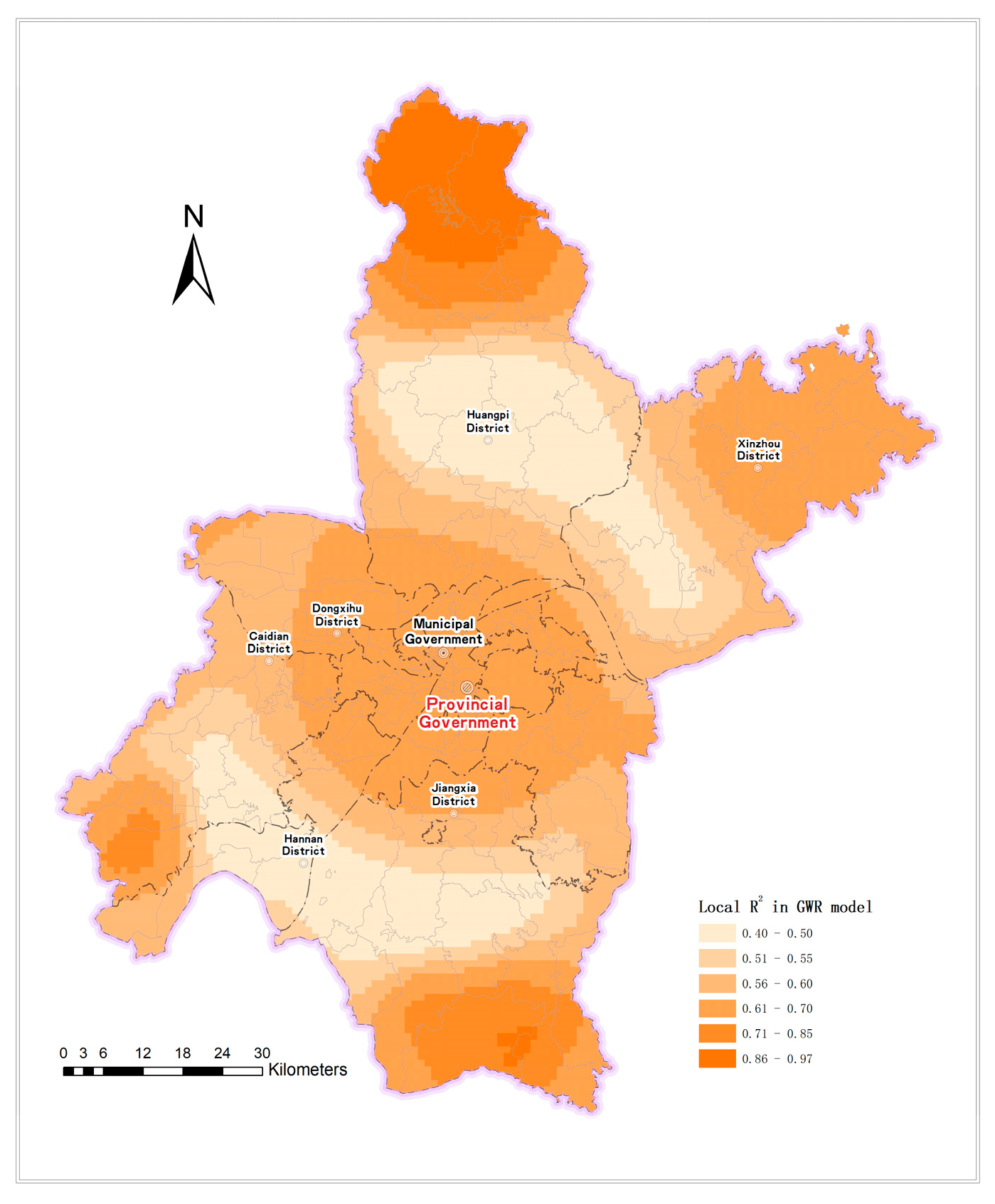
Figure 7.
GWR coefficient estimates of (a) Vegetation, (b) Water, (c) PrimaryIndustry, (d) TertiaryIndustry, (e) PerGDP, (f) RoadDensity, (g) BusDensity, (h) Construction.
Figure 7.
GWR coefficient estimates of (a) Vegetation, (b) Water, (c) PrimaryIndustry, (d) TertiaryIndustry, (e) PerGDP, (f) RoadDensity, (g) BusDensity, (h) Construction.


Table 1.
Classification of three industrial lands.
| Type of Industrial Land | Description |
|---|---|
| Primary Industry | Farmland in LCA |
| Secondary Industry | Industrial enterprises in urban intergrated functional units (BUCA) |
| Tertiary Industry | Service industry facilities, logistics and storage land in BUCA; construction sites in LCA |
Table 2.
Variable descriptions and statistics.
| Variable | Description | Unit | Min. | Max | |
|---|---|---|---|---|---|
| LRP | The land resource pressure index of each grid | 0.00 | 1.00 | ||
| Nature resources | Vegetation | Ratio of vegetation | 0.00 | 1.00 | |
| Water | Ratio of water | 0.00 | 1.00 | ||
| Economy | PrimaryIndustry | Added value of primary industry | 100 million/km2 | 0.00 | 0.99 |
| SecondaryIndustry | Added value of secondary industry | 1 billion/km2 | 0.00 | 1.02 | |
| TertiaryIndustry | Added value of tertiary industry | 1 billion/km2 | 0.00 | 3.41 | |
| PerGDP | Per capita gross domestic product | 10 million/person | 0.00 | 2.86 | |
| Transportation | RoadDensity | Road network density | 10 km/km2 | 0.00 | 1.43 |
| BusDensity | Bus lines density | 100 km/km2 | 0.00 | 0.96 | |
| SubCover | Ratio of 500-m subway buffer | 0.00 | 1.00 | ||
| Urban construction | Construction | Ratio of urban construction lands | 0.00 | 1.00 |
Table 3.
Classification criteria for suitable land.
| ID | Variable | Classification | Score | |
|---|---|---|---|---|
| 1 | SL | ≤3° | 100 | |
| 2 | 3°~8° | 80 | ||
| 3 | 8°~15° | 60 | ||
| 4 | 15~25° | 40 | ||
| 5 | >25° | 20 | ||
| 6 | EL | ≤500 m | 100 | |
| 7 | 500~1000 m | 80 | ||
| 8 | 1000~2000 m | 60 | ||
| 9 | 2000~3000 m | 40 | ||
| 10 | >3000 m | 20 | ||
| 11 | Basic farmland | 0 | ||
| 12 | Water or wetland | 0 | ||
| 13 | Lake reserve | 0 | ||
Table 4.
Summaries of GW correlation coefficients between LRP and its influence factors.
| Variables | Min. | Median | Max. | Max-Min | Mean |
|---|---|---|---|---|---|
| Vegetation | −0.919 | −0.286 | 0.490 | 1.408 | −0.252 |
| Water | −0.779 | −0.278 | 0.570 | 1.349 | −0.260 |
| PrimaryIndustry | −0.809 | −0.294 | 0.554 | 1.363 | −0.270 |
| SecondaryIndustry | −0.852 | 0.058 | 0.724 | 1.576 | −0.022 |
| TertiaryIndustry | −0.648 | 0.326 | 0.940 | 1.588 | 0.294 |
| PerGDP | −0.841 | −0.328 | 0.447 | 1.288 | −0.318 |
| RoadDensity | −0.186 | 0.611 | 0.897 | 1.082 | 0.596 |
| BusLinesDensity | −0.209 | 0.641 | 0.949 | 1.158 | 0.601 |
| SubCover | −0.415 | 0.388 | 0.967 | 1.382 | 0.352 |
| Construction | −0.877 | −0.143 | 0.670 | 1.547 | −0.142 |
Table 5.
Summarized information of the OLS and GWR results.
| Variables | GWR | OLS | ||
|---|---|---|---|---|
| Min. | Median | Max. | ||
| Intercept | −0.015 | 0.000 | 0.051 | −0.002 |
| Vegetation | −0.183 | −0.010 | 0.003 | −0.013 |
| Water | −0.093 | −0.001 | 0.009 | −0.007 |
| PrimaryIndustry | −0.004 | 0.006 | 0.034 | 0.010 |
| TertiaryIndustry | −0.223 | 0.029 | 0.213 | 0.038 |
| PerGDP | −0.683 | −0.065 | −0.016 | −0.037 |
| RoadDensity | −0.075 | −0.011 | 0.045 | −0.024 |
| BusDensity | −0.017 | 0.335 | 0.475 | 0.383 |
| Construction | 0.014 | 0.029 | 0.090 | 0.032 |
| AIC | −39,844.03 | −38,296.97 | ||
| AICc | −39,774.34 | −38,296.94 | ||
| R2 | 0.6197 | 0.5461 | ||
| Adjusted R2 | 0.6157 | 0.5457 | ||
© 2019 by the authors. Licensee MDPI, Basel, Switzerland. This article is an open access article distributed under the terms and conditions of the Creative Commons Attribution (CC BY) license (http://creativecommons.org/licenses/by/4.0/).
Share and Cite
MDPI and ACS Style
Yang, N.; Li, J.; Lu, B.; Luo, M.; Li, L. Exploring the Spatial Pattern and Influencing Factors of Land Carrying Capacity in Wuhan. Sustainability 2019, 11, 2786. https://doi.org/10.3390/su11102786
AMA Style
Yang N, Li J, Lu B, Luo M, Li L. Exploring the Spatial Pattern and Influencing Factors of Land Carrying Capacity in Wuhan. Sustainability. 2019; 11(10):2786. https://doi.org/10.3390/su11102786
Chicago/Turabian StyleYang, Nana, Jiansong Li, Binbin Lu, Minghai Luo, and Linze Li. 2019. "Exploring the Spatial Pattern and Influencing Factors of Land Carrying Capacity in Wuhan" Sustainability 11, no. 10: 2786. https://doi.org/10.3390/su11102786
Note that from the first issue of 2016, this journal uses article numbers instead of page numbers. See further details here.