Electricity Forecasting Improvement in a Destination Using Tourism Indicators


1
Departamento de Estadística e Investigación Operativa Aplicadas y Calidad, Universitat Politècnica de València, E46022 Valencia, Spain
2
Departamento de Dirección y Organización de Empresas, Universitat Politècnica de València, E46022 Valencia, Spain
*
Author to whom correspondence should be addressed.
Sustainability 2019, 11(13), 3656; https://doi.org/10.3390/su11133656
Submission received: 25 April 2019
/
Revised: 26 June 2019
/
Accepted: 28 June 2019
/
Published: 3 July 2019
(This article belongs to the Special Issue Sustainable Directions in Tourism)
Abstract
:The forecast of electricity consumption plays a fundamental role in the environmental impact of a tourist destination. Poor forecasting, under certain circumstances, can lead to huge economic losses and air pollution, as prediction errors usually have a large impact on the utilisation of fossil fuel-generation plants. Due to the seasonality of tourism, consumption in areas where the industry represents a big part of the economic activity follows a different pattern than in areas with a more regular economic distribution. The high economic impact and seasonality of the tourist activity suggests the use of variables specific to it to improve the electricity demand forecast. This article presents a Holt–Winters model with a tourism indicator to improve the effectiveness on the electricity demand forecast in the Balearic Islands (Spain). Results indicate that the presented model improves the accuracy of the prediction by 0.3%. We recommend the use of this type of model and indicator in tourist destinations where tourism accounts for a substantial amount of the Gross Domestic Product (GDP), we can control a significant amount of the flow of tourists and the electrical balance is controlled mainly by fossil fuel power plants.
1. Introduction
Tourism is growing worldwide, as is its environmental impact on tourist destinations. Evaluating the impact of tourism goes further than evaluating the economic facet; it must also take into account both its environmental and social dimensions [1,2]. Among the environmental dimensions, positive and negative impacts on biodiversity, erosion and physical damage, pollution, resources or landscape change have been reported [3]. The extent and nature of the environmental impact of tourism is related to the magnitude of the development and the volume of visitors, but also to the spatial and temporal concentration of tourism activities [4]. Thus, accurate forecasting of visitors allows to allocate the appropriate resources benefiting the sustainable development of tourism destinations [5]. Specifically, in the Balearic Islands, one of the main resources to manage is electricity. The vast majority of services require it to function, and have great economic and environmental impact.
Electricity demand management is a key factor—its development and use are increasing, both in terms of production and distribution. The efficiency of managing such resources has a big economic impact, as electricity powers a large amount of devices of any kind used. Energy cannot be stored in large quantities; rather, it must be produced on demand. Losses are generated when there is a mismatch between production and consumption. As energy is produced based on consumption prediction, reducing losses necessitates improving demand forecasts. A better prediction model will improve electricity production management.
The main objective of this paper is to present a new short-term prediction model for energy consumption that incorporates tourism indicators as a predictor. More precisely, we propose a new model that improves consumption prediction in an area where the tourism industry accounts for a big amount of the Gross Domestic Product (GDP), the Balearic Islands. Following Bakhat and Roselló [6], we incorporated Daily Human Pressure Indicator (DHPI). DHPI considers the variation on the population due to the increase or decrease of tourists. We hypothesised that the variation of the population in the tourism area is impacting the amount of electric energy consumed while other factors, such as temperature, remain constant. Therefore, introducing DHPI in a prediction model will improve significantly the energy consumption prediction.
The paper is structured as follows: in Section 2, we review the literature concerning the worked topics, in Section 3, we study the electrical demand in the Balearic Islands, and the associated emissions; in Section 4, we introduce the new model including a touristic indicator; in Section 5 we analyse the results and discuss them. Section 6 reflects on the conclusions and limitations of the study.
2. Literature Review
Research into the environmental impact of the tourism industry [7,8,9] has been focused primarily on determining the impact of transportation utilisation subserving it. Indeed, air transportation alone is believed to account for more than 60% of this impact. Scott et al. [10,11,12] analysed the tourism impact on Climate Change and Paris Agreement effects for the tourism industry.
Becken and Simmons [13] and Gössling [14,15] have described the potential environmental damage caused by tourism activities. Tourism impact on emissions has been reported by several authors (Meng et al. [16], Lee y Brahmasrene [17] Paramati et al. [18]). Specifically, tourism contributes approximately 5% to the global emissions of CO2 [19]. Important here is the increasing concern across countries about global warming, as is impacted by the latter. Such concerns extend to the energetic impact of tourism activities [20,21] as the industry represents one of the greatest energy consumers [7,13,15,22,23,24,25], especially in the European Union where travel and tourism represents the highest contributor to the GDP and visitors’ exports [26].
Studies have also paid attention to the hospitality industry ([16] Becken et al. [23,27]), a subsegment of tourism, as a primary energy consumer. World Tourism Organization and the United Nations Environment Programme estimated that accommodation accounts for 21% of tourism’s total greenhouse gas emissions [26].
Despite these worrisome indicators, the broadscale energy consumption and environmental pollution caused by tourism have not declined since the 1990s [10,11,28,29,30,31]. Pablo-Romero et al. [32], in fact, found an increasingly positive relationship between electricity consumption of the hospitality sector and overnight stays, and Katircioglu et al. [29] reported a positive relationship between tourist arrivals and energy consumption. Consequently, they recommended energy-efficiency measures, such as the adoption of renewable energy systems and the development of energy management capabilities. Moreover, the electricity consumption elasticity values of the hospitality sector (with respect to tourist overnight stays) have the highest values in touristic areas, indicating that for the same overnight stays the impact on electricity consumption is higher in these areas and, thus negatively affecting sustainability [33]. Other researchers [31,34,35] have indicated that provision of quality hotel service can produce increases in energy consumption.
The increase of tourism in certain areas is expected to increase the environmental impact on tourist destinations. Several initiatives have recently been undertaken by destination stakeholders to reduce its negative effects. These actions have focused mainly on governments setting environmental policy measures, setting objectives and providing financial support to reduce their carbon footprint [36] and tourism companies reducing energy and water consumption [37,38]. Following this line, there is still room for improvement within the actual technological system. More precisely, improving energy consumption prediction is able to reduce the environmental impact of energy utilisation and, at the same time, lower its overall cost.
Production management is also affected by generation units. Generation units are distributed between the available electrical production technologies that enable the electricity source to control the amount of production. Lags between demand and production turn out to be harmful to the environment, as they typically cause a higher use of fossil fuel-generation plants. When this occurs, carbon dioxide production from electricity production is increased, as is the cost of the energy. Hobbs [39] pointed out that a 1% prediction improvement can save thousands, even millions of dollars. More precisely, Hong [40] estimated that a 1% improvement in the short-term demand forecasting in an electrical system (based on 1GW peak demand) can save approximately $600,000 per year. Unfortunately, there is a research gap related to the evaluation of the environmental impact of this prediction inefficiency. However, using the Balearic Islands (Spain) consumption and emissions data from Red Eléctrica de España (Transmission system operator in Spain), we estimated that a 2% prediction error might be generating 1 T CO2/hour additional emissions.
3. Data
3.1. Electricity Demand and Their Emissions
Electricity management is a key factor in the Balearic Islands. Resources are limited, and a full power supply to citizens and industries must be ensured. The responsibility of this electricity distribution, as well as the operational planning of the production units and demand forecasting, is the responsibility of the Transmission System Operator (TSO). For that reason, Red Eléctrica de España (REE), the unique TSO in Spain, is always endeavouring to improve forecasting models to obtain more accurate predictions. REE continuously provides electricity demand in the Balearic Islands through the website www.ree.es. The overall electricity demand, forecasts and emissions can be obtained for each Island separately. They are provided in intervals of 10 min. In this paper, we developed the research model using an hourly resolution; this information was therefore cropped. We used available data from May 2013 to October 2015. Figure 1 shows the hourly electricity demand in Mallorca. Menorca’s demand provided similar results, but different from the peninsula.
The series shows effects that are highly influenced by the seasons, with maximum peaks occurring in summer and at the Easter holiday. This seasonality is mainly caused by tourism activity, as it is the main economic driver of the region. A comparison of the Islands’ Gross Domestic Product (GDP) and that of Spain, provided by Instituto Nacional e Estadística (INE) and Exceltur (main tourism non-profit group formed by 28 leading Spanish tourist groups), is shown in Figure 2. This accounts for the direct, indirect and induced effect on the GDP [41]. It can be easily shown how the tourism activity reaches up to 45% of the GDP in the Islands, whereas in Spain it only reaches 11%. In addition, the figure shows an increasing trend of this activity in the GDP from 2010. Thus, the more people coming into the Islands, the more consumption of electricity, as explained in the introduction.
Herce [42] analysed the economy in the Balearic Islands, as well as its electricity generation. He highlighted how between 1990 and 2005, CO2 emissions increased to 62.2%. This increase was due to the power usage of fossil fuel stations (which reached up to 97% of the produced energy in the Islands). The “Plan Director Sectorial Energético de la Illes Balears” [43], a sectorial energetic plan, promoted the construction of an interconnexion cable between the peninsula and the archipelago, as well as integration of renewables within the energy-generation system. However, as shown in Figure 3, the evolution of emissions is not yet under control. Emissions of CO2 are increasing as overall demand grows. However, more importantly, the emission factor (in T CO2/MWh) is also increasing (although its slope is less steep). The factor, altogether, reflects a worsening in the emissions objectives.
Figure 4 elucidates some of the primary factors causing emissions to continue their upward climb. Coal power stations represent half of the electrical generation. They are generally used as the main source, although other alternatives with less negative environmental impact are available. Renewables have a low generation ratio and, despite the green-focused policies, the ratio is still about 5%. The way to reduce this trend is to make greater investments in renewable energies [44]. In addition, a more useful and accurate electricity demand forecast would help to program the generation units (thereby enabling a change in the ratio of energy sources in favour of those that are renewable [45,46]).
The evolution of emissions and electricity demand shown in the previous figures reveal that the increasing trend is directly related to economic growth, and in particular to tourism activity. This is not an isolated case. Pfenninger and Keirstead [47] analysed several scenarios combining all kinds of energy sources in the UK. They concluded that there is no clear direction to be taken. There are still many constraints making fossil fuel power plants a source that needs to be exploited.
3.2. Daily Human Presure Indicator (DHPI)
Figure 5 shows data regarding arrivals and departures to and from the Islands, through both air- and seaports. It can be seen that tourist arrivals by ship and airplane exceed 20,000,000 passengers. The plot shows an increasing trend, due in part to local government policies [48,49]. Tourism can be expected to remain the main economic activity in the Island in the ensuing years.
However, these data cannot be directly integrated into a model. Both variables are dependent and cannot be worked separately. Nevertheless, the Institut d’Estadística de les Illes Balears (IBSTAT) publishes annual data regarding visitors to the Islands, obtained from data provided by the Balearic government (through an indicator named Daily Human Pressure Indicator; DHPI). This indicator measures the quantity of people in the Islands each day, incorporating tourists’ movements in the data. Riera and Mateu [50] explain how this indicator has been designed and the data are collected. The DHPI is defined according to a formula wherein (1),
where refers to the year of analysis; refers to the day of analysis. stands for the population on 1 January of the year ; represents the total arrivals (per sea and airport) to the Islands, whereas represents the departures. is the result of the difference between the year and the year . Finally, is considered the probability of making an error while estimating the arrivals. Figure 6 shows the evolution on within the years 1997 to 2017 for the main Islands Mallorca and Menorca.
The DHPI shows a high seasonal behaviour, with maximum peaks during summer, as the tourism in Balearic Islands is closely related to weather conditions [48]. An in-depth analysis of the indicator can reveal that the seasonality of electrical demand and DHPI are closely related. This point permits the DHPI to be integrated as part of an electricity demand model.
4. Model Development
Most TSOs use time series to model the behaviour of the electricity demand and price. This kind of tools have turned out to be very powerful as they provide very accurate predictions, although sometimes they are complex. Time series use the observed data in the past to fit a model, and later predict new values. Weron [51] gathers the state of the art of the techniques used for this purpose [52]. This author organises the forecasting methods in statistical methods, artificial intelligence and others. For the first group, representative methods are ARIMA models, exponential smoothing, including Holt–Winters methods, state space models and AR-models. The second group includes neural networks and support vector machines. Some other naïve methods are also available; however, their use is minor. TSOs usually develop their own models as a combination of all the former. In Spain, REE uses its own model in which 24 hourly subsets are forecasted each hour, and there is a daily forecast for medium-term purposes [53,54]. This model is based on the decomposition, for each hour of demand, in basic load (where trend and seasonality are included) and load modifiers due to special days or climatic factors. The basic load is adjusted to an ARIMA time series model, while the modifiers are dummy variables. Usually, TSOs do not publish their own forecasting models; they use a combination of several time series techniques, as described by Suganthi [55]. Electricité de France developed its own model based on regression models and Fourier decomposition of the seasonality [56,57], whereas TERNA (Italy’s TSO) uses a model more similar to REE’s [58,59].
This paper focuses on Holt–Winters’ methods, as they are very efficient in electricity demand forecasting, due to their simplicity and accuracy on time series with a strong seasonal effect [60].
4.1. Basic Holt–Winters Methods
The Holt–Winters exponential smoothing methods (HW) were introduced by P.R Winters [61] in the 1960s. These methods consist of several smoothing equations, which model the level, trend and seasonal components in the observed data. A final equation uses the information of smoothing equations to provide forecasts, and thus, it is named forecasting equation. In all models, there is at least one level equation. The other equations can be avoided if no trend or no seasonality is considered. Equations (2)–(5) show the Holt–Winters model.
where is the level equation with a smoothing parameter α, stands for the trend equation, with smoothing parameter γ and is the seasonal indices of cycle length and smoothing parameter δ. is the observed data whereas is the k-ahead predictions; is the adjustment factor related to the first autocorrelation error (). Gardner et al. [62] and latterly Taylor [63] include a damping factor in the trend. Williams and Miller [64] propose a new model in which interventions are modelled as level adjustments. The most important evolution is introduced by J.W. Taylor by including the double [65] and triple seasonal [66] Holt–Winters (HWT), and an adjustment using the first autocorrelation error (AR1), that improves the forecasts [67]. Trull et al. use discrete-interval moving seasonalities to model Easter holidays [68].
The equations in the model can be combined using different methods: additive and multiplicative. The previous methods used an additive method for trends, while seasonal indices were included using a multiplicative one. García-Díaz and Trull [69] generalise these methods to n seasonalities and apply them using three factors followed by the seasonal cycle length. The first factor stands for the trend method, the second for the seasonal method, and the third describes whether the model has been adjusted with AR1. Table 1 summarises all possible combinations. As an example, a 24 h-length multiplicative trend, multiplicative seasonality including AR1 adjustment will expressed as MMC24.
The parameters are obtained through an optimisation algorithm, by minimising the error of a one-step-ahead forecast compared to observed values. The Holt–Winters methods are recursive; it is thus mandatory to obtain at the beginning the initial values of each model. The level was obtained as the moving average of the first two cycles. The trend was calculated by averaging the difference between the first and the second cycle. The seasonal indices were obtained by dividing each value of the first cycle by moving average. The minimisation algorithm is then launched, with the smoothing parameters bounded between 0 and 1. The root of the mean of the squared error (RMSE) is used to measure the error. RMSE is defined in Equation (6).
where is the number of observed values in the time series used to fit the model.
4.2. New Holt–Winters with the DHPI Model
The first autocorrelation error obtained during the model fit, as a result of the optimisation, reflects the variability of the series itself, but also could be related to another exogenous variable. The addition of the AR1 adjustment improves the forecasting accuracy, but some information could be lost. The innovation proposed in this paper consists in splitting this error into two components: one due to the effect of the variability by tourism indicators and the other due to the variability of the series itself. It is possible to perform this action because, as explained in the introductory section, the energy use of the Balearic Islands is highly related to tourism; it is also geographically aisled.
The air temperature is an exogenous variable that is commonly integrated into the model(s) used [70], but, for very short-term forecasting, it is not necessary. The demand itself captures the temperature transitions [71]. Only abrupt changes in the climate conditions could have influence on the model; however, the temperature in Balearic Islands is relatively smooth and thus can be considered constant. In the same way, GDP is a variable that must be kept out of the model. While it may have influence in the long term [72], it is not possible to include it in the model. The series correspond to the aggregate demand of all energy of the islands, and not only that related to tourism. However, the fact that tourism has such a high percentage of GDP means that demand must be associated with tourism components, such as the DHPI, contrary to other places where the weight of tourism is not so high, and its effect is diluted among other sectors. A good sample is the peninsula, where the industrial sector exerts its influence.
The procedure to integrate the indicator in the model was as follows: First, we obtained a simple Holt–Winters model for the DHPI without AR1 adjustment, as the error will be used in the main model. We used the Holt–Winters model for DHPI because the time series shows a high seasonal component and is proportional to the demand model. The DHPI model is described by Equations (7)–(10).
where , and are the equations for level, trend and seasonal indices with smoothing parameters , and for the DIPH. are the k-ahead prediction values for DHPI. The error made by the forecasts of (10) is a very important information. The model defined by (2)–(5) does not react to forecasts produced by (10) because that information is latent in the model. However, a big difference between the forecast of (10) and DHPI means a special situation, that the model (2)–(5) cannot adequately describe or account for. We tried using covariates, as explained by Bermúdez [73], but the results were not positive. The way to relate mismatches in the both forecasting equations—demand and DHPI—is through a linear combination, as shown in (11).
Here, is the relation factor between both models. The complete model is thus expressed as in Equations (12)–(19).
In order to exploit the model, variables should match on the resolution. Electricity demand is provided hourly, while DHPI is daily. This discrepancy is solved by using 24 hourly models for electricity demand, one for each hour, that share the same DHPI. That is, we used 24-h models to forecast every day.
5. Results
In order to check the effectiveness of the new proposed model, we tested all methods in Table 1. An analysis was carried out, in which the forecasts for the electricity demand for Mallorca and Menorca were validated. We split the available data into two subsets: we used 90% of the observed values to fit the models and obtain the parameters, and the rest to perform an out-of-sample validation, making forecasts and comparing with real values.
To obtain the new parameter , we tested two different methods, as it was not clear which one could be more efficient:
- two-step process, where both models were fit separately to obtain the parameters. Then, parameters were combined to obtain .
- The DHPI was initially fit, as the electricity demand model requires its error. After obtaining DHPI parameters and error, the complete model is simultaneously adjusted, including .
The forecast accuracy for m-ahead forecasts was measured using the Mean Average Percentage Error (MAPE) defined in (20).
The validation process of the method consists in making forecasts for a specific horizon, and comparing them with the real data obtained a posteriori during a period. This period is chosen according to whether it is sufficiently representative [74,75]. We used a forecast horizon of 24 h (typical for the short-term forecasting) during a period of 7 days, as tourists’ average stay in the Island is about 8 days (source: IBESTAT). The analysis compared the MAPE obtained using the basic model against the new proposal. The average improvement obtained for Mallorca and Menorca is summarized in Table 2. Although all methods in Table 1 were tested, only the most relevant are shown in Table 2. The new proposal outperforms the basic model as it reduces MAPE. The best results are obtained in Mallorca, as the tourist population is much bigger in Mallorca, as is its influence on the results. Additionally, we decided to apply for further analysis the all-in-one method as it outperformed the two-step one.
Based on the former results, we focused the analysis on the Mallorca electricity demand, and we built Table 3. It shows an hourly split of the MAPE improvement against the basic model. The main improvements are produced during the central hours of the day. These results might be indicating the relation between the energy consumption and tourists’ activity. Our results indicate that the proposed model can reach an improvement of 0.3% in MAPE. This results in an estimated reduction of 200 kg CO2/hour.
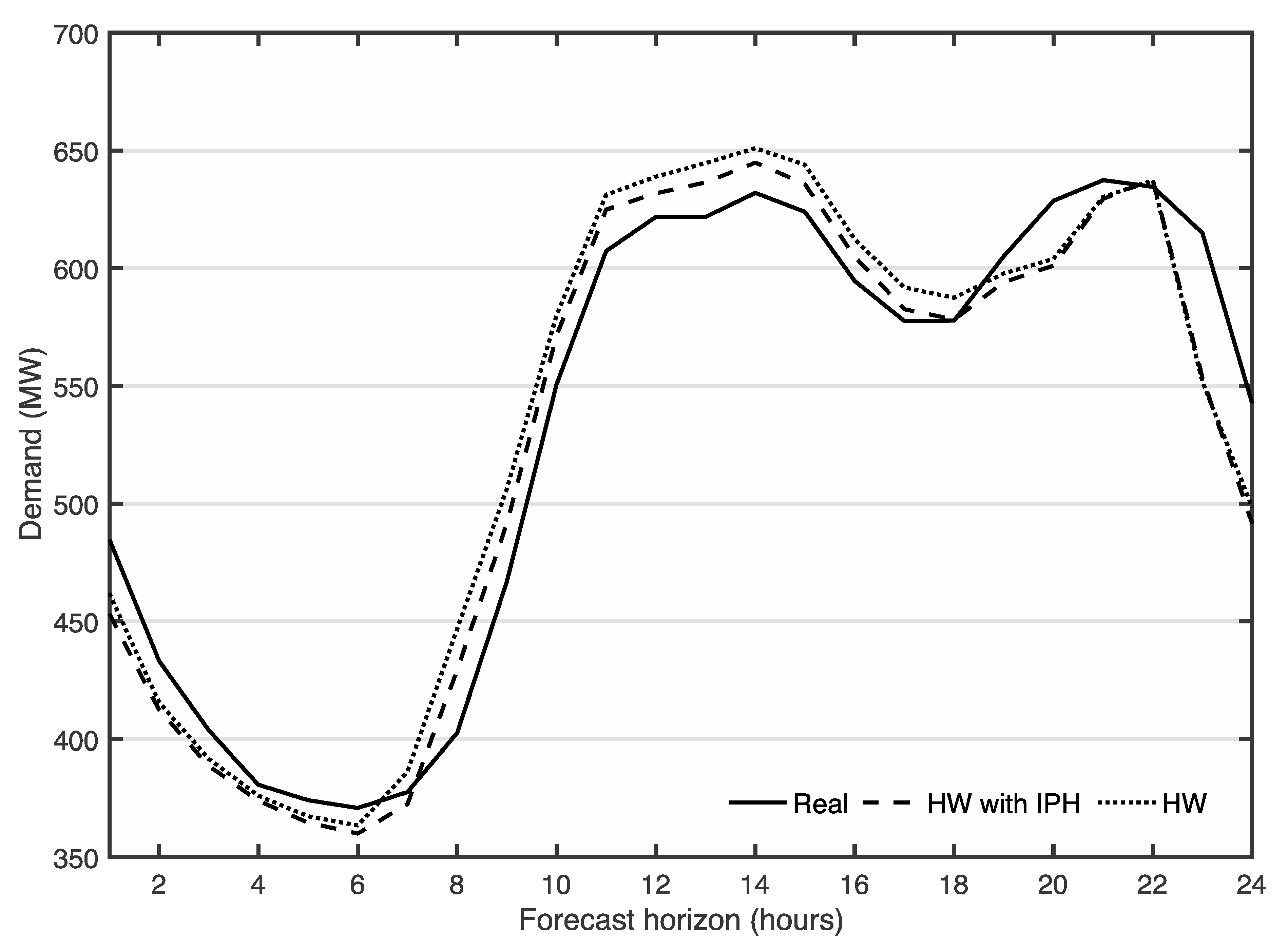
Figure 7 shows a comparison chart for a random day between the demand forecasts given by the regular HW model and the proposed new model. It is appreciated as the new proposal outperforms the results, and approaches the real demand. This graph shows how the introduction of the DHPI acts in the model, bringing the forecast closer to the real demand compared to the regular model. In any case, it is a random example, and at other times the result may be different, although on average the improvements indicated in Table 3 will be obtained.
6. Conclusions and Limitations
Tourism has been a powerful tool for local destination development, however social concern about its environmental impact is raising questions about the overall benefits of touristic activities at a local level [76]. The associated environmental costs related to the tourism industry have a broad scope that needs specific approaches [3].
In this paper, we work on the reduction of the environmental impact due to the electricity consumption. More specifically, we focus on electricity demand forecast. The aim of electricity prediction improvement is to reduce the economic and environmental impact caused by forecast errors on electricity demand. Particularly, the environmental impact due to the generation of greenhouse gases has been continuously increasing, despite the policies carried out to increase renewable energies [19]. This effect, in the electricity system, is caused mainly by the generation structure. The generation system uses coal and diesel power plants to adapt to the demand. Demand errors increase the production of these power plants and consequently, the pollution.
We followed Cardenas and Roselló [5], introducing the Daily Human Pressure Indicator, which relates the arrivals and departures of passengers on a daily basis. Previous findings about the relation of energy consumption with tourism pressure [29,32], a higher electricity consumption elasticity in touristic areas [32] and the greater portion of the total electricity consumption due to tourism activities suggested the use of tourism indicators to improve the electricity forecast in tourism areas. Then, the introduction of DHPI makes sense in a context where tourism-related activities represent a large portion of the local GDP. We analyse the demand and its relationship with tourism in the Balearic Islands where tourism accounts for up to 45% of the GDP. Data indicates that electricity demand time series are highly affected by the tourist variation. Thus, we developed a new model using DHPI to improve forecasts. We present a new electric demand forecast model using the Holt–Winters model. We checked the effectiveness of the new model using the data provided by REE and IBESTAT. The results indicated that the model improves demand predictions up to 0.3% in MAPE. This improvement would allow the TSO plan and supply a larger amount of the electricity from sustainable sources and its impact would be equivalent to a reduction in CO2 emissions of around 200 Kg/hour.
Our study contributes to uncover the benefits of using relevant indicators related to the dominant economic activity in an area to improve the electricity consumption forecast. The results have relevant implications to TSO providers and policy makers. TSO providers might improve the electric consumption forecast at a local level with data sources outside the electricity sector. Policy makers might encourage the data exchange between public institutions and TSO to improve the forecast and reduce the environmental impact. Moreover, policy makers might use information from electricity consumption and tourism activity to evaluate the impact of environmental policies and actions taken in a touristic area.
The analysis of this model has been limited to the Balearic Islands, in which tourism accounts for a large portion of the GDP and DHPI is easily associated with the electricity demand as it is calculated by the human arrival to and departure from the islands by sea or by air. The use of these indicators in other tourist destinations might be limited by the number of these visitors accessing the area by other means, such as car or train. However, this might be an interesting path for specific destinations where tourist flow is easily controlled and the electrical balance is controlled by fossil fuel power plants. Future research will have to verify this model in other similar tourist destinations, such as the Canary Islands, to strengthen our conclusions.
Author Contributions
Conceptualization, O.T. and A.P.-S.; Formal analysis, O.T. and J.C.G.-D.; Investigation, O.T.; Methodology, O.T.; Software, O.T.; Writing—original draft, O.T. and A.P.-S.; Writing—review and editing, O.T., A.P.-S. and J.C.G.-D.
Funding
This research received no external funding.
Acknowledgments
The authors would like to thank the editor and the four anonymous referees for their thorough comments and suggestions. We would also like to thank Institut d’Estadística de les Illes Balears (IBESTAT) for providing DHPI data.
Conflicts of Interest
The authors declare no conflict of interest.
References
- Gray, R.; Bebbington, J. Accounting for the Environment; Sage Publications: London, UK, 2001; ISBN 9780761971368. [Google Scholar]
- Rubio Gil, M.Á.; Mazón Martínez, T. El capital social como factor coadyuvante de los procesos de desarrollo turístico y socioeconómico de los destinos de interior [Social capital as a contributory factor in the tourism and socioeconomic development processes of interior destinations]. Pap. Tur. 2009, 45, 41–55. [Google Scholar]
- Mason, P. Tourism Impacts, Planning and Management, 3rd ed.; Routledge: London, UK, 2015; ISBN 9781315781068. [Google Scholar]
- Archer, B.; Cooper, C.; Ruhanen, L. The positive and negative impacts of tourism. In Global Tourism; Elsevier Science: Burlington, MA, USA, 2005; pp. 79–102. [Google Scholar]
- Zhang, M.; Li, J.; Pan, B.; Zhang, G. Weekly hotel occupancy forecasting of a tourism destination. Sustainability 2018, 10, 4351. [Google Scholar] [CrossRef]
- Bakhat, M.; Rosselló, J. Estimation of tourism-induced electricity consumption: The case study of Balearics Islands, Spain. Energy Econ. 2011, 33, 437–444. [Google Scholar] [CrossRef]
- Gössling, S. Sustainable Tourism Development in Developing Countries: Some Aspects of Energy Use. J. Sustain. Tour. 2000, 8, 410–425. [Google Scholar] [CrossRef]
- Gössling, S.; Hall, M. An Introduction to Tourism and Global Environmental Change. In Tourism and Global Environmental Change; Routledge: London, UK, 2006; pp. 15–48. ISBN 9780203011911. [Google Scholar]
- Peeters, P.; Schouten, F. Reducing the Ecological Footprint of Inbound Tourism and Transport to Amsterdam. J. Sustain. Tour. 2006, 14, 157–171. [Google Scholar] [CrossRef]
- Scott, D.; Hall, C.M.; Gössling, S. A report on the Paris Climate Change Agreement and its implications for tourism: Why we will always have Paris. J. Sustain. Tour. 2016, 24, 933–948. [Google Scholar] [CrossRef]
- Scott, D.; Hall, C.M.; Gössling, S. A review of the IPCC Fifth Assessment and implications for tourism sector climate resilience and decarbonization. J. Sustain. Tour. 2016, 24, 8–30. [Google Scholar] [CrossRef]
- Scott, D.; Gössling, S.; Hall, C.M.; Peeters, P. Can tourism be part of the decarbonized global economy? The costs and risks of alternate carbon reduction policy pathways. J. Sustain. Tour. 2016, 24, 52–72. [Google Scholar] [CrossRef]
- Becken, S.; Simmons, D.G. Understanding energy consumption patterns of tourist attractions and activities in New Zealand. Tour. Manag. 2002, 23, 343–354. [Google Scholar] [CrossRef]
- Gössling, S. Global environmental consequences of tourism. Glob. Environ. Chang. 2002, 12, 283–302. [Google Scholar] [CrossRef]
- Gössling, S.; Hansson, C.B.; Hörstmeier, O.; Saggel, S. Ecological footprint analysis as a tool to assess tourism sustainability. Ecol. Econ. 2002, 43, 199–211. [Google Scholar] [CrossRef]
- Meng, W.; Xu, L.; Hu, B.; Zhou, J.; Wang, Z. Quantifying direct and indirect carbon dioxide emissions of the Chinese tourism industry. J. Clean. Prod. 2016, 126, 586–594. [Google Scholar] [CrossRef]
- Lee, J.; Brahmasrene, T. Investigating the influence of tourism on economic growth and carbon emissions: Evidence from panel analysis of the European Union. Tour. Manag. 2013, 38, 69–76. [Google Scholar] [CrossRef]
- Paramati, S.R.; Alam, M.S.; Chen, C.-F. The Effects of Tourism on Economic Growth and CO2 Emissions: A Comparison between Developed and Developing Economies. J. Travel Res. 2017, 56, 712–724. [Google Scholar] [CrossRef]
- Rutty, M.; Gössling, S.; Scott, D.; Hall, C.M. The Global Effects and Impacts of Tourism. In The Routledge Handbook of Tourism and Sustainability; Routledge: Abingdon, UK, 2015. [Google Scholar]
- Cárdenas, V.; Rosselló, J. Análisis económico de los impactos del cambio climático en el turismo: Estado de la cuestión [Economic analysis of the impacts of climate change on tourism: State of the art]. Ekonomiaz Revista vasca de Economía 2008, 67, 262–283. [Google Scholar]
- Fortuny, M.; Soler, R.; Cánovas, C.; Sánchez, A. Technical approach for a sustainable tourism development. Case study in the Balearic Islands. J. Clean. Prod. 2008, 16, 860–869. [Google Scholar] [CrossRef]
- Becken, S. Analysing international tourist flows to estimate energy use associated with air travel. J. Sustain. Tour. 2002, 10, 114–131. [Google Scholar] [CrossRef]
- Becken, S.; Simmons, D.G.; Frampton, C. Energy use associated with different travel choices. Tour. Manag. 2003, 24, 267–277. [Google Scholar] [CrossRef]
- Becken, S. Tourism and Transport in New Zealand: Implications for Energy Use. 2001, pp. 1–34. Available online: https://core.ac.uk/download/pdf/35459093.pdf (accessed on 21 January 2019).
- Tabatchnaia-Tamirisa, N.; Loke, M.K.; Leung, P.; Tucker, K.A. Energy and tourism in Hawaii. Ann. Tour. Res. 1997, 24, 390–401. [Google Scholar] [CrossRef]
- World Tourism Organization and the United Nations Environment Programme (Ed.) Climate Change and Tourism-Responding to Global Challenges; World Tourism Organization and the United Nations Environment Programme: Madrid, Spain, 2008; ISBN 9789284412341. [Google Scholar]
- Becken, S.; Frampton, C.; Simmons, D. Energy consumption patterns in the accommodation sector—The New Zealand case. Ecol. Econ. 2001, 39, 371–386. [Google Scholar] [CrossRef]
- Katircioglu, S.T. International tourism, energy consumption, and environmental pollution: The case of Turkey. Renew. Sustain. Energy Rev. 2014, 36, 180–187. [Google Scholar] [CrossRef]
- Katircioglu, S.T.; Feridun, M.; Kilinc, C. Estimating tourism-induced energy consumption and CO2 emissions: The case of Cyprus. Renew. Sustain. Energy Rev. 2014, 29, 634–640. [Google Scholar] [CrossRef]
- Zaman, K.; Shahbaz, M.; Loganathan, N.; Raza, S.A. Tourism development, energy consumption and Environmental Kuznets Curve: Trivariate analysis in the panel of developed and developing countries. Tour. Manag. 2016, 54, 275–283. [Google Scholar] [CrossRef]
- Tsai, K.T.; Lin, T.P.; Hwang, R.L.; Huang, Y.J. Carbon dioxide emissions generated by energy consumption of hotels and homestay facilities in Taiwan. Tour. Manag. 2014, 42, 13–21. [Google Scholar] [CrossRef]
- Pablo-Romero, M.d.P.; Pozo-Barajas, R.; Sánchez-Rivas, J. Relationships between tourism and hospitality sector electricity consumption in Spanish Provinces (1999–2013). Sustainability 2017, 9, 480. [Google Scholar]
- Pablo-Romero, M.P.; Sánchez-Braza, A.; Sánchez-Rivas, J. Relationships between hotel and restaurant electricity consumption and tourism in 11 European Union countries. Sustainability 2017, 9, 2109. [Google Scholar] [CrossRef]
- Wang, J.C. A study on the energy performance of school buildings in Taiwan. Energy Build. 2016, 133, 810–822. [Google Scholar] [CrossRef]
- Warnken, J.; Bradley, M.; Guilding, C. Eco-resorts vs. mainstream accommodation providers: An investigation of the viability of benchmarking environmental performance. Tour. Manag. 2005, 26, 367–379. [Google Scholar] [CrossRef]
- Financing Europe’s Low Carbon, Climate Resilient Future. Available online: https://www.eea.europa.eu/themes/climate/financing-europe2019s-low-carbon-climate (accessed on 12 May 2019).
- Pace, L.A. How do tourism firms innovate for sustainable energy consumption? A capabilities perspective on the adoption of energy efficiency in tourism accommodation establishments. J. Clean. Prod. 2016, 111, 409–420. [Google Scholar] [CrossRef]
- Sozer, H. Improving energy efficiency through the design of the building envelope. Build. Environ. 2010, 45, 2581–2593. [Google Scholar] [CrossRef]
- Hobbs, B.F. Analysis of the value for unit commitment of improved load forecasts. IEEE Trans. Power Syst. 1999, 14, 1342–1348. [Google Scholar] [CrossRef]
- Hong, T. Crystal Ball Lessons in Predictive Analytics. Energybiz 2015, 12, 35–37. [Google Scholar]
- Polo, C.; Valle, E. Un análisis estructural de la economía balear [A structural analysis of the Balearic economy]. Estadística Española 2007, 49, 227–257. [Google Scholar]
- Herce, J.A. La economía de Illes Balears: Diagnóstico estratégico [The Economy of Illes Balears: Strategic Diagnosis]; SE La Caixa: Barcelona, Spain, 2008. [Google Scholar]
- BOIB. Aprobación Definitiva de la Revisión del Plan Director Sectorial Energético de las Illes Balears. [Final Approval of the Revision of the Sectorial Energy Management Plan of the Balearic Island]; Consejería de Comercio, Industriay Energía: Mallorca, Spain, 2005; pp. 46–53. [Google Scholar]
- Bilan, Y.; Streimikiene, D.; Vasylieva, T.; Lyulyov, O.; Pimonenko, T.; Pavlyk, A.; Bilan, Y.; Streimikiene, D.; Vasylieva, T.; Lyulyov, O.; et al. Linking between Renewable Energy, CO2 Emissions, and Economic Growth: Challenges for Candidates and Potential Candidates for the EU Membership. Sustainability 2019, 11, 1528. [Google Scholar] [CrossRef]
- Morales, J.M.; Conejo, A.J.; Madsen, H.; Pinson, P.; Zugno, M. Integrating Renewables in Electricity Markets: Operational Problems; Springer: New York, NY, USA, 2013; ISBN 9781461494119. [Google Scholar]
- Sioshansi, F. Evolution of Global Electricity Markets: New Paradigms, New Challenges, New Approaches; Elsevier Science & Technology: Amsterdam, The Netherlands, 2013; ISBN 9780123979063. [Google Scholar]
- Pfenninger, S.; Keirstead, J. Renewables, nuclear, or fossil fuels? Scenarios for Great Britain’s power system considering costs, emissions and energy security. Appl. Energy 2015, 152, 83–93. [Google Scholar] [CrossRef]
- Aguiló, E.; Alegre, J.; Sard, M. The persistence of the sun and sand tourism model. Tour. Manag. 2005, 26, 219–231. [Google Scholar] [CrossRef]
- Manera, C. El creixement de l’economia turística a les Illes [The growth of the tourist economy in the Islands]. Recerques 2009, 59, 151–192. [Google Scholar]
- Riera Font, A.; Mateu Sbert, J. Aproximación al volumen de turismo residencial en la Comunidad Autónoma de las Illes Balears a partir del cómputo de la carga demográfica real [Approximation to the volume of residential tourism in the Autonomous Community of the Balearic Islands from the calculation of the real demographic burden]. Estud. Turísticos 2007, 174, 59–71. [Google Scholar]
- Weron, R. Modeling and Forecasting Electricity Loads and Prices: A Statistical Approach; John Wiley & Sons: Chichester, UK, 2006; ISBN 978-0-470-05753-7. [Google Scholar]
- Weron, R. Electricity price forecasting: A review of the state-of-the-art with a look into the future. Int. J. Forecast. 2014, 30, 1030–1081. [Google Scholar] [CrossRef] [Green Version]
- Cancelo, J.R.; Espasa, A.; Grafe, R. Forecasting the electricity load from one day to one week ahead for the Spanish system operator. Int. J. Forecast. 2008, 24, 588–602. [Google Scholar] [CrossRef] [Green Version]
- López, M.; Valero, S.; Senabre, C.; Gabaldón, A. Analysis of the Influence of Meteorological Variables on Real-Time Short-Term Load Forecasting in Balearic Islands. In Proceedings of the 2017 11th IEEE International Conference on Compatibility, Power Electronics and Power Engineering, CPE-POWERENG 2017, Cadiz, Spain, 4–6 April 2017; Institute of Electrical and Electronics Engineers Inc.: Cádiz, Spain, 2017; pp. 10–15. [Google Scholar]
- Suganthi, L.; Samuel, A.A. Energy models for demand forecasting—A review. Renew. Sustain. Energy Rev. 2012, 16, 1223–1240. [Google Scholar] [CrossRef]
- Bruhns, A.; Deurveilher, G.; Roy, J. A non-linear regression model for mid-term load forecasting and improvements in seasonality. In Proceedings of the PSCC’05, Liège, Belgium, 22–26 August 2005; pp. 22–26. [Google Scholar]
- Pierrot, A.; Goude, Y. Short-Term Electricity Load Forecasting With Generalized Additive Models. In Proceedings of the 16th Intelligent System Applications to Power Systems Conference (ISAP), Hersonisso, Greece, 25–28 September 2011. [Google Scholar]
- Bianco, V.; Manca, O.; Nardini, S. Electricity consumption forecasting in Italy using linear regression models. Energy 2009, 34, 1413–1421. [Google Scholar] [CrossRef]
- De Felice, M.; Alessandri, A.; Ruti, P.M. Electricity demand forecasting over Italy: Potential benefits using numerical weather prediction models. Electr. Power Syst. Res. 2013, 104, 71–79. [Google Scholar] [CrossRef]
- Taylor, J.W. An evaluation of methods for very short-term load forecasting using minute-by-minute British data. Int. J. Forecast. 2008, 24, 645–658. [Google Scholar] [CrossRef]
- Winters, P.R. Forecasting sales by exponentially weighted moving averages. Management 1960, 6, 324–342. [Google Scholar]
- Gardner, E.S.; McKenzie, E., Jr.; McKenzie, E. Forecasting Trends in Time Series. Manag. Sci. 1985, 31, 1237–1246. [Google Scholar] [CrossRef]
- Taylor, J.W. Exponential smoothing with a damped multiplicative trend. Int. J. Forecast. 2003, 19, 715–725. [Google Scholar] [CrossRef] [Green Version]
- Williams, D.W.; Miller, D. Level-adjusted exponential smoothing for modeling planned discontinuities. Int. J. Forecast. 1999, 15, 273–289. [Google Scholar] [CrossRef]
- Taylor, J.W. Short-term electricity demand forecasting using double seasonal exponential smoothing. J. Oper. Res. Soc. 2003, 54, 799–805. [Google Scholar] [CrossRef]
- Taylor, J.W. Triple seasonal methods for short-term electricity demand forecasting. Eur. J. Oper. Res. 2010, 204, 139–152. [Google Scholar] [CrossRef] [Green Version]
- Gardner, E.S., Jr. Exponential smoothing: The state of the art, part II. Int. J. Forecast. 2006, 22, 637–666. [Google Scholar] [CrossRef]
- Trull, Ó.; García-Díaz, J.C.; Troncoso, A.; Trull, Ó.; García-Díaz, J.C.; Troncoso, A. Application of Discrete-Interval Moving Seasonalities to Spanish Electricity Demand Forecasting during Easter. Energies 2019, 12, 1083. [Google Scholar] [CrossRef]
- García-Díaz, J.C.; Trull, Ó. Competitive Models for the Spanish Short-Term Electricity Demand Forecasting. In Time Series Analysis and Forecasting: Selected Contributions from the ITISE Conference; Rojas, I., Pomares, H., Eds.; Springer International Publishing: Cham, Germany, 2016; pp. 217–231. ISBN 978-3-319-28725-6. [Google Scholar]
- Pardo, A.; Meneu, V.; Valor, E. Temperature and seasonality influences on Spanish electricity load. Energy Econ. 2002, 24, 55–70. [Google Scholar] [CrossRef]
- Taylor, J.W.; McSharry, P.E. Short-term load forecasting methods: An evaluation based on european data. Power Syst. IEEE Trans. 2007, 22, 2213–2219. [Google Scholar] [CrossRef]
- Pérez-García, J.; Moral-Carcedo, J. Analysis and long term forecasting of electricity demand trough a decomposition model: A case study for Spain. Energy 2016, 97, 127–143. [Google Scholar] [CrossRef]
- Bermúdez, J.D. Exponential smoothing with covariates applied to electricity demand forecast. Eur. J. Ind. Eng. 2013, 7, 333–349. [Google Scholar] [CrossRef]
- Hyndman, R.J.; Athanasopoulos, G. Forecasting: Principles and Practice; OTexts: Melbourne, Australia, 2018; ISBN 978-0-9875071-1-2. [Google Scholar]
- Bergmeir, C.; Hyndman, R.J.; Koo, B. A Note on the Validity of Cross-Validation for Evaluating Autoregressive Time Series Prediction. Comput. Stat. Data Anal. 2018, 120, 70–83. [Google Scholar] [CrossRef]
- Almeida García, F.; Balbuena Vázquez, A.; Rafael, C.M. Resident’s attitudes towards the impacts of tourism. Tour. Manag. Perspect. 2015, 13, 33–40. [Google Scholar] [CrossRef]
Figure 1.
Hourly electricity demand in Mallorca.

Figure 2.
Tourism Gross Domestic Product (GDP) in the Balearic Islands against Spain’s. Source: Own elaboration based on Incotur’s and Exceltur’s information.
Figure 2.
Tourism Gross Domestic Product (GDP) in the Balearic Islands against Spain’s. Source: Own elaboration based on Incotur’s and Exceltur’s information.

Figure 3.
Evolution of the CO2 emissions in the Balearic Islands due to power generation. The emissions factor is measured as a weight of emissions per MWh, right axis.
Figure 3.
Evolution of the CO2 emissions in the Balearic Islands due to power generation. The emissions factor is measured as a weight of emissions per MWh, right axis.
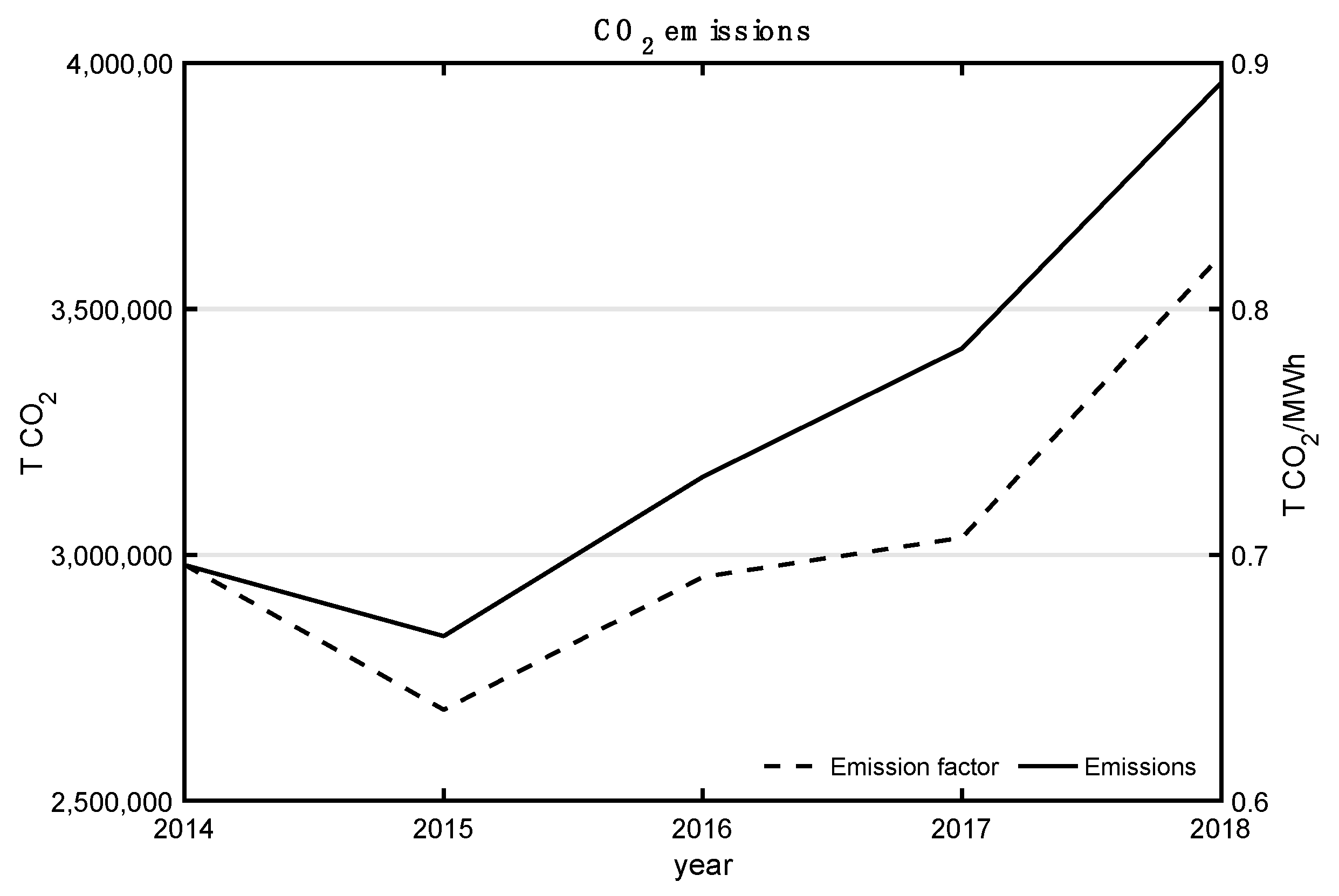
Figure 4.
Distribution of the electricity generation in the Balearic Islands.
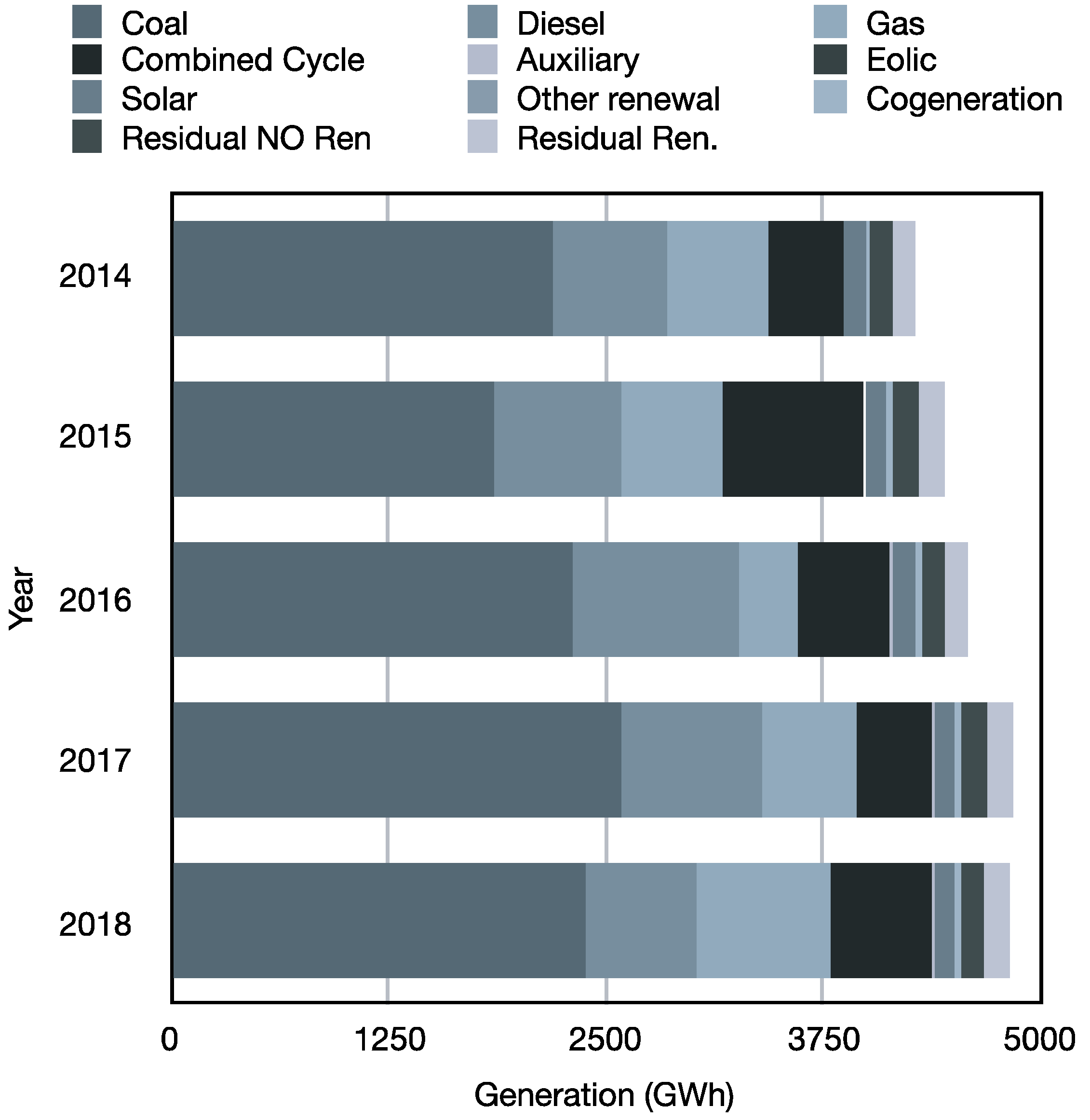
Figure 5.
Balance of arrivals and departures to/from Balearic Islands. (a) seaport data; (b) airport data. Source: IBSTAT.
Figure 5.
Balance of arrivals and departures to/from Balearic Islands. (a) seaport data; (b) airport data. Source: IBSTAT.
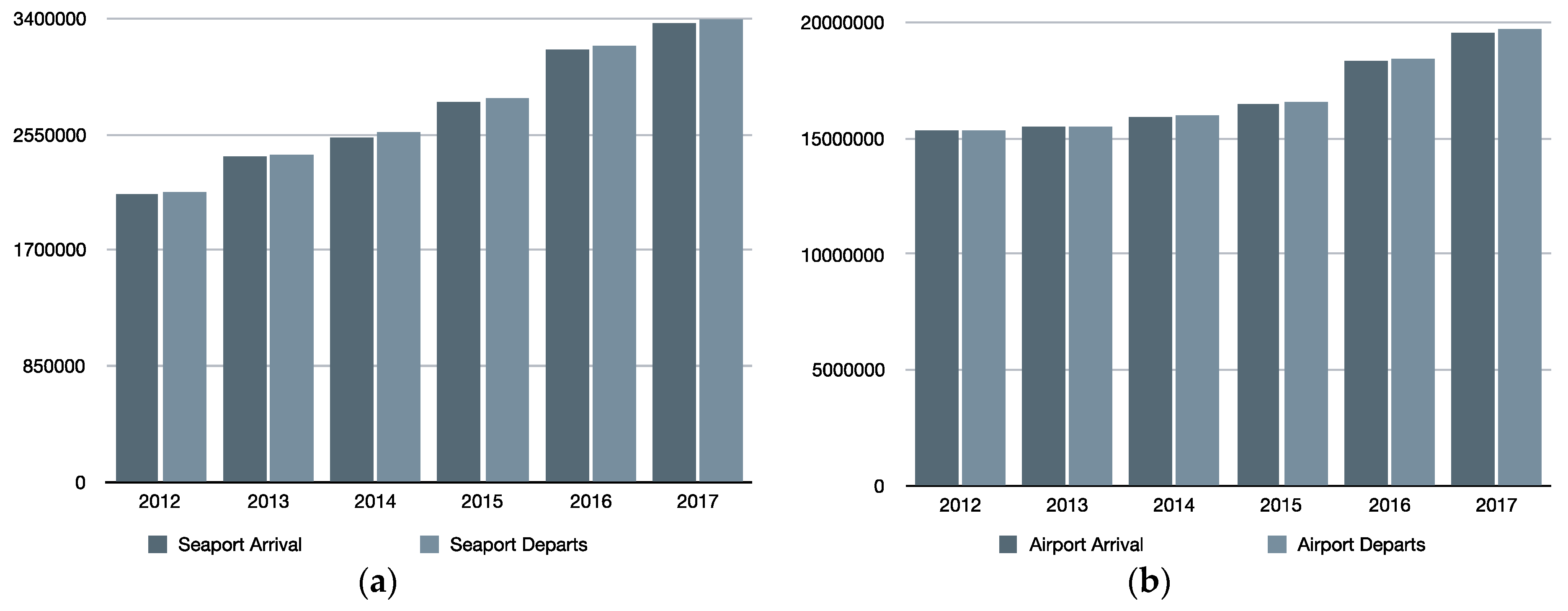
Figure 6.
Daily human pressure index in Mallorca and Menorca. Source: IBESTAT.

Figure 7.
Comparison of one-day-ahead forecasts using the HW method and the new proposed HW-IPH, against the real consumption.
Figure 7.
Comparison of one-day-ahead forecasts using the HW method and the new proposed HW-IPH, against the real consumption.

Table 1.
Summary of Holt–Winters (HWT) method combinations.
| Seasonality | None | Additive | Multip. | None | Additive | Multip. | |
|---|---|---|---|---|---|---|---|
| Trend | Normal | AR(1) Adjusted | |||||
| None | NNL | NAL | NML | NNC | NAC | NMC | |
| Additive | ANL | AAL | AML | ANC | AAC | AMC | |
| Damped Additive | dNL | dAL | dML | dNC | dAC | dMC | |
| Multiplicative | MNL | MAL | DML | MNC | MAC | MMC | |
| Damped Multiplicative | DNL | DML | DML | DMC | DAC | DMC | |
Table 2.
Forecast comparison of the new proposal against the standard method. Average reduction of the hourly MAPE% for 7-days-ahead forecasts in Mallorca and Menorca.
Table 2.
Forecast comparison of the new proposal against the standard method. Average reduction of the hourly MAPE% for 7-days-ahead forecasts in Mallorca and Menorca.
| Mallorca | Menorca | |||
|---|---|---|---|---|
| 2-STEP | ALL-IN-ONE | 2-STEP | ALL-IN-ONE | |
| AMC | −0.06 | −0.12 | −0.03 | −0.02 |
| AAC | −0.05 | −0.10 | −0.03 | −0.03 |
| NAC | −0.05 | −0.09 | −0.03 | −0.03 |
| NMC | −0.06 | −0.11 | −0.03 | −0.03 |
Table 3.
Hourly MAPE reduction in the electricity forecasting for Mallorca. A comparison among the selected models.
Table 3.
Hourly MAPE reduction in the electricity forecasting for Mallorca. A comparison among the selected models.
| Hour | AMC | AAC | NAC | NMC |
|---|---|---|---|---|
| 1 | 0.0 | 0.0 | 0.0 | 0.0 |
| 2 | −0.1 | 0.0 | 0.0 | 0.0 |
| 3 | 0.0 | 0.0 | 0.0 | 0.0 |
| 4 | 0.0 | 0.0 | 0.0 | 0.0 |
| 5 | 0.0 | 0.0 | 0.0 | 0.0 |
| 6 | 0.0 | 0.0 | 0.0 | 0.0 |
| 7 | −0.1 | −0.1 | −0.1 | −0.1 |
| 8 | −0.3 | −0.2 | −0.2 | −0.3 |
| 9 | −0.2 | −0.2 | −0.2 | −0.2 |
| 10 | −0.1 | −0.1 | −0.1 | −0.1 |
| 11 | −0.1 | −0.1 | −0.1 | −0.1 |
| 12 | −0.2 | −0.1 | −0.1 | −0.2 |
| 13 | −0.1 | −0.1 | −0.1 | −0.1 |
| 14 | −0.1 | −0.1 | −0.1 | −0.1 |
| 15 | −0.1 | −0.1 | −0.1 | −0.1 |
| 16 | −0.2 | −0.2 | −0.2 | −0.2 |
| 17 | −0.2 | −0.2 | −0.2 | −0.2 |
| 18 | −0.3 | −0.2 | −0.2 | −0.2 |
| 19 | −0.2 | −0.2 | −0.2 | −0.2 |
| 20 | −0.2 | −0.2 | −0.2 | −0.2 |
| 21 | −0.2 | −0.2 | −0.2 | −0.2 |
| 22 | −0.1 | −0.1 | −0.1 | −0.1 |
| 23 | 0.0 | 0.0 | 0.0 | 0.0 |
| 24 | −0.1 | −0.2 | 0.0 | 0.0 |
© 2019 by the authors. Licensee MDPI, Basel, Switzerland. This article is an open access article distributed under the terms and conditions of the Creative Commons Attribution (CC BY) license (http://creativecommons.org/licenses/by/4.0/).
Share and Cite
MDPI and ACS Style
Trull, O.; Peiró-Signes, A.; García-Díaz, J.C. Electricity Forecasting Improvement in a Destination Using Tourism Indicators. Sustainability 2019, 11, 3656. https://doi.org/10.3390/su11133656
AMA Style
Trull O, Peiró-Signes A, García-Díaz JC. Electricity Forecasting Improvement in a Destination Using Tourism Indicators. Sustainability. 2019; 11(13):3656. https://doi.org/10.3390/su11133656
Chicago/Turabian StyleTrull, Oscar, Angel Peiró-Signes, and J. Carlos García-Díaz. 2019. "Electricity Forecasting Improvement in a Destination Using Tourism Indicators" Sustainability 11, no. 13: 3656. https://doi.org/10.3390/su11133656
Note that from the first issue of 2016, this journal uses article numbers instead of page numbers. See further details here.