Innovation Search Scope, Technological Complexity, and Environmental Turbulence: A N-K Simulation

1
College of Public Administration, Zhejiang University, Hangzhou 310058, China
2
School of Economics and Management, Tsinghua University, Beijing 100084, China
3
School of Business Administration, Zhejiang University of Finance and Economics, Hangzhou 310018, China
*
Author to whom correspondence should be addressed.
Sustainability 2019, 11(16), 4279; https://doi.org/10.3390/su11164279
Submission received: 11 July 2019
/
Revised: 31 July 2019
/
Accepted: 5 August 2019
/
Published: 7 August 2019
(This article belongs to the Section Economic and Business Aspects of Sustainability)
Abstract
:This paper discusses the effects of different innovation search scopes on the performance of the N-K fitness landscape model with a focus on its contextual factors of technology complexity and environmental turbulence. Results show that the medium-level search scope has a significantly better outcome than the low-level search scope, especially when the technological complexity is high, while the high-level search scope would not provide a statistically significant advantage. After introducing the turbulent range and rapidity into the N-K model, we extend the model into a dynamic one to simulate better the real turbulent business world. The results of the simulation in dynamic landscapes show that the higher degree of environmental turbulence causes a higher search scope to become more valuable.
1. Introduction
Innovation search, which is defined as “a problem-solving activity in which firms solve problems through combining knowledge elements to create new products (pp. 88)” [1], has attracted increasing attention from both academics and practice. Following the views of Nelson and Winter [2], Katila and Ahuja [3] introduced the concept of innovation search scope, which is generally defined as how widely the firm explores new knowledge. Developing the open innovation theory proposed by Chesbrough [4], which could also be considered as part of innovation search, Laursen and Salter [5] proposed a similar concept named as external search breadth. Based upon these concepts, extant literature has focused mainly on the value of higher innovation search scope [6,7,8,9], while environmental and technological contingencies are largely ignored.
In fact, issues of technological complexity, which are defined as the degree of interdependence among components in a technological system [10], have been recognized as critically important to the ability of firms to manage innovation successfully [10,11]. Meanwhile, environmental turbulence, which refers to those market or technological changes that are frequent and unpredictable [12], has significance in the innovation search process, particularly for firms in transitional economies, such as China [13,14].
This paper develops a theoretical model on innovation search scope by considering the moderating effects of environmental turbulence and technology complexity with the N-K adaptive landscape method. In our paper, innovation search scope is operationalized as the number of technological components developed simultaneously during the innovation process. Each technology could be considered as a system with interdependent components and thus, it is suitable for use in analyzing the process of technology innovation by the N-K model [15], which allows us to compare the different levels of innovation search scope. Our argument starts with the observation that during the innovation process, some firms choose to treat technology components one by one, while others deal with several components simultaneously. By increasing the innovation search scope, some firms achieve much better performance, while others face problems. Thus, examining whether firms should expand their innovation search scope is an interesting step. Interactions and interdependence between technological components are constantly observed, and thus, the answer is not a simple “the larger, the better.” However, if the innovation search scope is indeed valuable, what about its contextual factors? According to our reviews and observations, technological complexity and environmental turbulence might be as two essential factors, which would influence the effect of the innovation search scope on innovation performance.
Using the formal N-K model, we examine the relationship between innovation search scope and performance as well as the moderating effects of technological complexity and environmental turbulence. The simulation results show that in a stable environment, a firm could expect significant performance improvement by expanding its Innovation Search Scope from low to medium level in accordance to the research of scholars, such as Katila and Ahuja [3] and Laursen and Salter [5]. With regard to technological complexity, we determined that the improvement increases with the increase in complexity and that the high-level innovation search scope is more valuable than the medium level only if the technology is with great complexity. Firms with higher innovation search scope could expect significantly better innovation performance with the increase in its technological complexity.
Our research contributes to the literature in the following ways. First, we further develop the N-K fitness landscape simulation model [16,17] by introducing the environmental turbulence more concretely. As an important simulation tool, the N-K model has been used widely in studies in the fields of innovation, strategic management, and organization [18,19]. Several studies [17] have considered changing environments. That is, once N and K are fixed, the typology of the fitness landscape will not change with time. In reality, however, the value of certain technology continues to change because of the emergence of new technology, changes in customer’s preferences, and industrial structure. We extend the N-K model into a dynamic model by introducing two turbulence variables. This paper is expected to optimize the simulation for the changing environment by introducing two variables: turbulent rapidity and turbulent range. In our dynamic landscapes, we find that the expansion of the innovation search scope becomes more valuable as the turbulence increases, which means a firm with a larger search scope could achieve better improvement in the turbulent environment, compared to that in more stable one. This paper also focuses on the value of innovation search scope and its contextual factors, which has not been given sufficient focus. During the technology innovation process, firms could deal with the technological components one by one or several components simultaneously. Dealing with the technological components becomes even more complicated when factors, such as technological complexity and environmental turbulence, set in. Our paper takes these determinants into consideration and studies how they jointly influence innovation performance.
The paper is organized as follows. We review the concept and effect of technological complexity and environmental turbulence in the following section. We then present our model and describe the mechanics of the simulations. Finally, we present and analyze the results and make conclusions.
2. Literature Review
2.1. Innovation Search
Innovation search refers to the problem-solving activity in which firms solve problems by combining knowledge components to create new products, better organization form, or operation process [3,20,21]. The knowledge sources for innovation search includes both internal and external [22]. Through the analysis of the robot industry, Katila and Ahuja [3] empirically proved the existence of an inverted U-shaped relationship between the innovation search scope and new product performance. Zhang and Li [1] focused on external search, particularly on the role of intermediary institutes. Generally, extant literature has agreed that a firm can obtain higher innovation performance when broader innovation sources are searched [6,7,8,9]. However, few studies have focused on the contextual factors of innovation search scope—innovation performance relationship, especially the moderating role of Environmental Turbulence and technological complexity.
2.2. Technological Complexity
Defining and understanding technological complexity is the premise for analyzing its influence on innovation and business. The concept of complexity is described in many fields, spanning natural and manmade systems in manufacturing, computer systems and organizational structures [23,24,25]. Similar to the concept of complex systems [26], technology is also composed of structured components. Knowledge complexity is the origin of technological complexity and is defined as the number and interaction of interdependent components, routines, individuals, and resources [27]. Simon [26] classifies knowledge as complex if it is composed of many elements that interact richly. Higher degree interdependence indicates that many ingredients influence the effectiveness of others so that an improvement in one may dramatically reduce the usefulness of the system [21]. Garud and Nayya [28] considered the knowledge complexity from the view of information: the greater complexity of knowledge, the greater the uncertainty and the need to collect more information to make choices and the greater the amount of information that must be maintained and retrieved over time.
Therefore, we define technological complexity as the degree of interdependence among components in a technological system. Technological complexity plays an important role in innovation [10,29]. The problem with increasing technological complexity during the innovation process is that it causes more difficulty in getting things done. Integrated technology components cause difficulty in the transformation into a successful product or process innovation [30]. Engineers have to spend their time trying to predict, avoid, and debug the subtle interdependences among components rather than exploring new combinations [23]. Thus, innovators might face a complex catastrophe when they attempt to combine highly interdependent technologies [31]. Technological opportunities would also increase with complexity, and thus, innovators can take advantage of increasing sensitivities and opportunistic couplings among components [23,31]. In fact, Baldwin and Clark [32] argue that the optimal degree of interdependence lies where we could achieve the balance between uncertainty and complexity.
2.3. Environmental Turbulence
The innovation processes are environmentally context-dependent [33,34,35]. Emery and Trist [36] first proposed the concept of environmental turbulence. From then on, environmental turbulence has been described in many different ways: unfamiliar [37], hostile and heterogeneous [38], uncertainty [39], complexity [40], and dynamic [38,41]. We followed Calantone et al. [42] and defined environmental turbulence as that in which market or technological changes are frequent and unpredictable. Market and technology are two main aspects of environmental turbulence [12,43]. Market turbulence refers to the degree of instability and uncertainty within a firm’s market, while technological turbulence refers to the rate of technological change [14,44,45,46,47].
We argue that the essence of environmental (both market and technology) turbulence’s effect on the firm is that it makes firm’s knowledge (including technology) evolve [46,48,49]. In other words, because of the environmental turbulence, the value of the same technology may increase or decrease with time. Consequently, the contribution of technology to innovation performance fluctuates. We define environmental turbulence as the rapidity and range of the market and technological changes that would vary the value of firm knowledge (including technology) [50]. Rapidity and range of environmental turbulence are two key factors determined by industry features, stage of the industry life cycle, and technology evolution. We take four industries as an example to differentiate better the range and rapidity. Figure 1 shows that new energy is a novel industry with high turbulent rapidity and range, while textile is a mature one with low rapidity and range. As for the pharmacy industry, it remains relevantly stable and does not change very frequently. However, whenever a change occurs in the pharmacy industry, it must be a radical one, which is why pharmacy is located in the upper right corner. In contrast, the cellphone industry [42] is fast-paced, evolves rapidly, and does not undergo a radical change.
3. The Dynamic N-K Model
3.1. Baseline Model
Since Kauffman [16] introduced the N-K model into the study of biological evolution, the model has been applied widely by innovation scholars to simulate the complex system of management [17,18,19]. Technology is also a complex system with interdependent components and hence, using the N-K model is suitable for use in simulating the technology innovation process [15]. Our formal baseline model is as follows:
where we assume a technology system is composed of N interdependent components represented by a vector of <b1, b2, …, bn>, where each bi is an element of {0,1}.
The contribution ci of each component bi to system performance depends on other K components. Thus, K represents the degree of complexity in the system. For each of 2K possible combinations, a value is drawn from a uniform probability distribution on [0,1] [18].
The performance of the entire technology system is average over the N contributions. Hence, we can generate a landscape with 2N performance values.
For a specific firm, it would have an initial vector <b1…,bi…, bN> with performance P. During each simulation period, firm changes any one component bi into bi’, to generate a new vector <b1…,bi’…, bN> with performance P’. If P’ is bigger than P, the firm will move the new position where b’ is in the configuration. If the P’ is less than P, it will return to the initial position where b is in the configuration. This process is called the hill-climbing adaptive walk. By adopting this process, the firm would keep moving until it reaches an optimal peak in the landscape.
3.2. Innovation Search Scope
In most of the studies that apply N-K models [51], only one component bi will be changed at each time to activate the adaptive walk. In one period, a firm would look at alternatives that are only one step away from their current position and select the best alternatives [18]. In this case, a firm pays attention each time to one technology component to try to improve the overall performance, called “incremental improvement search” or “greedy search”. A firm can only walk one step nearby in the fitness landscape because of the search narrowness. When it reaches a peak, a higher probability that firm would be trapped in this so-called “sub-optima” position, not the global peak, exists simply because the one-step adaptive walk cannot make the organization “jump” to other higher peaks [16].
In reality, however, we see many cases with “radical improvement search”, where firms would improve more than one technological component simultaneously. Thus, the N-K model needs to be extended. In line with Rivkin and Siggelkow’s research [19], we introduce s (innovation search scope: technology innovation scope) into our model, which is the number of components that can be changed in every period. For example, s = 5 means a firm can try to mutate five components simultaneously; for instance, from (00000000) to (01011011) in just a one-time period. Through this step, we can find the effect of the search scope on the performance. Different from the study by Rivkin and Siggelkow [19], we also let the firm “climb” in a dynamic fitness landscape.
3.3. Simulation
In all our simulations, we set N = 12, while K has six options: 1, 3, 5, 7, 9, and 11, to represent the different levels of technological complexity. The higher the K, the more rugged the landscape would be [16]. In the first step, we release 12 firms in stable landscape and each firm has a search scope (the variable s) ranging from 1 to 12 to represent different levels of search scopes. Each simulation lasts for 200 periods. By doing this for 30 times, we might find whether a statistically significant difference can be found between the performances of different search scopes. The effect of complexity (K) was also examined.
Next, the 12 firms would be released into our dynamic landscape by setting t = 2 and r = 0.12. We need to analyze t and r separately to further find the effect of environmental turbulence. Thus, by keeping K = 5 and t = 6, we simulate the four combinations of (t, r)—(2, 0.12), (2, 0.02), (10, 0.12) and (10, 0.02), to represent four types of environmental turbulence—(high rapidity, large range), (high rapidity, small range), (low rapidity, large range), and (low rapidity, small range). All the simulations were 200-period for 30 times.
3.4. Dynamics of Landscape
Our simulation extends the traditional N-K fitness landscapes model. In most prior studies, the landscape is stable. That is, given a specific combination of N and K, the landscape is fixed without any change with time. As discussed in the previous sections, in the real business world, the value of knowledge or technology would change with time because of t environmental turbulence. Thus, the N-K landscape should be dynamic to realize better simulation [17].
We fluctuate the landscape by introducing variables t and r into the model to reflect the key factors of environmental turbulence, rapidity and range and to capture the effect of turbulence as simply as possible. In our model, the landscape would change randomly within certain simulation period intervals, and t refers to the period interval when the simulator activates the landscape changes. For example, t = 2 means the landscape itself will change every two periods. Thus, the larger t, the lesser the rapidity. Meanwhile, r reflects the change range of landscape in the simulations. Suppose the contribution of certain component b0 equals to c0 at the time t0, it would change randomly at time t0 + t in our model and the simulator will randomly pick up a value from [c0 − r, c0 + r], to give a new contribution c0’ of the same b0. Thus, the turbulent range would become larger by increasing r. Taking t = 5 and r = 0.05 as an example, if a technology component has a contribution c = 0.6 in time period t1, a new contribution c’ is picked randomly up from an interval [0.6 − 0.05, 0.6 + 0.05] in time period t1 + 5.
Two main differences can be observed between our dynamic landscape simulation and prior stable one. In the stable one, the overall value of technology would never diminish but could increase and decrease in the dynamic one. Obviously, the later one could better simulate the real world because no value of technology continues upwards all the time. There is also no need for a fixed optimal peak in the dynamic one because the landscape fluctuates with time. Hence, we will measure the average performance of all time periods to compare the result, instead of the last performance in the stable one [18,51]. Figure 2 shows that in a stable landscape, performance rises and remains steady one it reaches the optimal peak, while in our dynamic landscape, performance fluctuates.
4. Results
4.1. Simulation Results in Stable Landscape
We attempted to analyze the effects of innovation search scopes on innovation performance in a stable landscape. In our simulation process, we have 12 different scopes, ranging from 1 to 12. Different from Rivkin and Siggelkow [19], we do not think the comparison of a certain number of scopes make sense. Thus, we divided all 12 scopes into three groups, low scope (1 to 4), medium scope (5 to 8), and high scope (9 to 12), and conduct the t-test on the differences between the three groups. All the normality is checked before the ANOVA.
Table 1 shows that the mean differences between medium and low scopes are statistically significant in all levels of technological complexity, except for K = 1 when the complexity is very low. That is, when the technological complexity is not that low, the firm could expect a significantly higher performance by increasing its innovation search scope from low to medium. We also calculate the advantage percentage of medium scope on low, which is listed in the parentheses, to compare the effects of complexity. As the K increased from 3 to 5, 7, 9, and 11, the advantage percentage expanded from 5.15% to 6.06%, 6.86%, 8.14%, and 11.2%, respectively, with statistical significance. Thus, high technological complexity can make the medium scope more valuable.
In terms of the differences between high and medium scopes, statistical significance exists only in cases of high-level complexity (K = 9 and 11). Hence, a high search scope might not ensure significant performance improvement. Only when the technology is very complex could a firm expect performance advantage by enlarging the search scope from medium to high. The effect of complexity can still be determined because the advantage percentage increases with K. Comparing the second and third rows in Table 1, we also could find that the advantage of high as against medium is much less than that of medium on low, which means that the positive effect of search scope on innovation performance decreases as search scope enlarged.
Therefore, we might conclude that in the stable landscapes, the firm could realize significantly higher innovation performance by enlarging its technology innovation scope from low level to medium (unless the technology is much less complex), and high technology complexity would make the enlargement more valuable. The advantage of high compared to medium is statistically significant only in the case of high-level complexity.
4.2. Simulation Results in Dynamic Landscape
Next, we will examine the effect of Innovation Search Scopes in dynamic landscapes. Innovation Search Scope would also be divided into three groups. But this time, variables t and r are introduced into our model. Setting t = 2 and r = 0.12 (high rapidity and large range), we make the N-K fitness landscape dynamic. Before the analysis with ANOVA, we also examine the normality of data.
According to Table 2, there are statistically significant advantages of medium scope on low, in all levels of complexity, including the case of K = 1, which is different from the result in stable landscapes. As the complexity increases (K, from 1 to 11), the advantage percentage (numbers in the parenthesis) grows (from 3.08% to 10.4%), which means that high complexity makes the medium scope more valuable in the turbulent environments, too. As to the differences between high scope and medium, the statistical significance exists in the cases of not only high-level complexity (K = 9 and 11) but also medium-level complexity (K = 5 and 7). This means that it is more valuable to enlarge the search scope from medium to high in turbulent environments.
In order to better compare the advantage differences in dynamic and stable landscapes, we put them into the same figure (regardless of statistical significance here). Figure 3 shows the advantage percentage of medium scope on low both in dynamic and stale landscapes, which Figure 4 shows that of high scope on medium. We might determine clearly from the two figures that the advantage percentages are larger in a dynamic landscape than a stable landscape in all levels of complexity. Thus, in a dynamic landscape, higher technology innovation scope is more valuable for firms.
The differences between dynamic landscape and stable landscape interest us to further examine the effect of environmental turbulence, by analyzing t and r separately. We constructed four combinations of t and r: (2, 0.02), (2, 0.12), (10.0.02) and (10, 0.012). By comparing the advantage percentages in the four situations, we try to make the effect of environmental turbulence clear.
Figure 5 and Figure 6 show that the advantage percentage becomes larger as the turbulent rapidity or range increases. The advantage percentage was the largest in a situation with high rapidity and large range (7.48% and 2.08%), and least in a situation with low rapidity and small range (5.01%, 0.51%). The results shown in the two matrices above confirm that both turbulent rapidity and range make the enlargement of technology innovation scope more valuable. Turbulent rapidity and range had positive effects on the relationship between innovation search scope and innovation performance.
5. Conclusions
Using the formal N-K simulation method [17,18,19], the effect of innovation search scope on innovation performance in the stable landscapes is examined by introducing the innovation search scope into our model [19]. The simulation results show that firms could expect a significant improvement in their innovation performance by increasing their innovation search scope from a low to a medium level. A higher technological complexity causes the improvement to become larger, which means a medium scope is more valuable in high complexity context. However, no statistical significance was observed between high and medium scopes, unless the technology has very high complexity. This finding further proves the effect of technological complexity on the relationship between innovation search cope and innovation performance.
We make the fitness landscape dynamic to simulate reality better [17]. Thus, we extend the traditional N-K model by introducing two variables, t for turbulent rapidity and r for turbulent range. Using the turbulence matrix, we find that both turbulent rapidity and turbulent range have a positive effect on the advantage percentage of higher scope. That is, higher innovation search scope would be more valuable in an environment with higher rapidity or larger range and bring a larger advantage. Firms in a turbulent environment, such as new energy in Figure 1, should make full use of the greater profit from the higher innovation search scope.
These findings have important managerial implications. First, firms could expect a considerably higher performance by expanding its innovation search scope to a medium level. Compared to ones that adopt the “incremental search strategy”, “radical search” firms could achieve much better innovation performance; however, “the more, the better” is necessarily true. The positive effect of innovation search scope on performance decreases and the advantages of high scope on the medium are usually not significant. Thus, medium-level innovation search scope is suitable for most firms. Second, technological complexity makes the higher scope more valuable. Hence, firms in the industry with high technological complexity, such as computer and automobile, should focus more on the enlargement of innovation search scope. Moreover, compared to the results in a stable landscape, all the advantage percentage improves. Meanwhile, the performance differences between high and medium scopes become more significant in the dynamic landscape. A firm could achieve better innovation performance by expanding innovation search scope from medium to high, as long as the technological complexity is low. Therefore, the enlargement of the innovation search scope is more valuable in a turbulent environment such as China [1,52,53,54].
This paper extends the traditional N-K model to make it dynamic by introducing turbulent rapidity and turbulent range, which better simulates the real world. However, dynamic N-K fitness landscape should be developed further to make it more reasonable and reliable. The method of simulation has some typical deficiencies that could be improved through the use of other methods, such as a case study.
Author Contributions
Conceptualization, J.C. and F.L.; methodology, F.L. and Y.Y.; formal analysis, F.L. and Y.Y.; writing, F.L. and Y.Y., funding acquisition, Y.Y.
Funding
This research was funded by Zhejiang Province Philosophy and Social Sciences Project, grant number 19NDJC154YB; National Natural Science Foundation of China, grant number: 71874150.
Conflicts of Interest
The authors declare no conflict of interest. The funders had no role in the design of the study; in the collection, analyses, or interpretation of data; in the writing of the manuscript, or in the decision to publish the results.
References
- Zhang, Y.; Li, H. Innovation search of new ventures in a technology cluster: The role of ties with service intermediaries. Strat. Manag. J. 2010, 31, 88–109. [Google Scholar] [CrossRef]
- Nelson, R.R.; Winter, S.G. A Evolutionary Theory of Economic Change; Harvard University Press: Cambridge, MA, USA, 1982. [Google Scholar]
- Katila, R.; Ahuja, G. Something Old, Something New: A Longitudinal Study of Search Behavior and New Product Introduction. Acad. Manag. J. 2002, 45, 1183–1194. [Google Scholar]
- Chesbrough, H.W. Open Innovation: The New Imperative for Creating and Profiting from Technology; Harvard Business School Press: Boston, MA, USA, 2003. [Google Scholar]
- Laursen, K.; Salter, A. Open for innovation: The role of openness in the explaining innovation performance among UK manufacturing firms. Strateg. Manag. J. 2006, 27, 131–150. [Google Scholar] [CrossRef]
- Ren, S.; Eisingerich, A.B.; Tsai, H.-T. Search scope and innovation performance of emerging-market firms. J. Bus. Res. 2015, 68, 102–108. [Google Scholar] [CrossRef]
- Ying, Y.; Liu, Y.; Cheng, C. R&D activities dispersion and innovation: Implications for firms in China. Asian J. Technol. Innov. 2016, 24, 361–377. [Google Scholar]
- Wu, A.; Wei, J. Effects of Geographic Search on Product Innovation in Industrial Cluster Firms in China. Manag. Organ. Rev. 2013, 9, 465–487. [Google Scholar] [CrossRef]
- Wu, H.; Liu, Y. Balancing local and international knowledge search for internationalization of emerging economy multinationals. Chin. Manag. Stud. 2018, 12, 701–719. [Google Scholar] [CrossRef]
- Yayavaram, S.; Chen, W.R. Changes in firm knowledge couplings and firm innovation performance: The moderating role of technological complexity. Strateg. Manag. J. 2015, 36, 377–396. [Google Scholar] [CrossRef]
- Rycroft, R.W.; Kash, D.E. The Complexity Challenge: Technological Innovation for the 21st Century; Pinter: London, UK; New York, NY, USA, 1999. [Google Scholar]
- Droge, C.; Calantone, R.; Harmancioglu, N. New Product Success: Is It Really Controllable by Managers in Highly Turbulent Environments? J. Prod. Innov. Manag. 2008, 25, 272–286. [Google Scholar] [CrossRef]
- Wei, J.; Wang, D.; Liu, Y. Towards an asymmetry-based view of Chinese firms’ technological catch-up. Front. Bus. Res. China 2018, 12, 20. [Google Scholar] [CrossRef]
- Liu, Y.; Deng, P.; Wei, J.; Ying, Y.; Tian, M. International R&D alliances and innovation for emerging market multinationals: Roles of environmental turbulence and knowledge transfer. J. Bus. Ind. Mark. 2019. [Google Scholar] [CrossRef]
- Giannoccaro, I.; Nair, A.; Choi, T. The impact of control and complexity on supply network performance: An empirically informed investigation using NK simulation analysis. Decis. Sci. 2018, 49, 625–659. [Google Scholar] [CrossRef]
- Kauffman, S.A. The Origins of Order; Oxford University Press: New York, NY, USA, 1993. [Google Scholar]
- Levinthal, D.A. Adaptation on Rugged Landscapes. Manag. Sci. 1997, 43, 934–950. [Google Scholar] [CrossRef]
- Almirall, E.; Casadesus-Masanell, R. Open Versus Closed Innovation: A Model of Discovery and Divergence. Acad. Manag. Rev. 2010, 35, 27–47. [Google Scholar]
- Rivkin, J.W.; Siggelkow, N. Patterned interactions in complex systems: Implications for exploration. Manag. Sci. 2007, 53, 1068–1085. [Google Scholar] [CrossRef]
- Katila, R. New product research over time: Past ideas in their prime? Acad. Manag. J. 2002, 45, 995–1010. [Google Scholar] [CrossRef]
- Sorenson, O.; Rivkin, J.W.; Fleming, L. Complexity, networks and knowledge flow. Res. Policy 2006, 35, 994–1017. [Google Scholar] [CrossRef]
- Chen, J.; Chen, Y.; Vanhaverbeke, W. The influence of scope, depth, and orientation of external technology sources on the innovative performance of Chinese firms. Technovation 2011, 31, 362–373. [Google Scholar] [CrossRef] [Green Version]
- Chong, W.K.; Bian, D.; Zhang, N. E-marketing services and e-marketing performance: The roles of innovation, knowledge complexity and environmental turbulence in influencing the relationship. J. Mark. Manag. 2016, 32, 149–178. [Google Scholar] [CrossRef]
- MacDuffie, J.P.; Sethuraman, K.; Fisher, M.L. Product Variety and manufacturing Performance: Evidence from the international Automotive Assembly Plant Study. Manag. Sci. 1996, 42, 350–369. [Google Scholar] [CrossRef]
- Okwir, S.; Nudurupati, S.S.; Ginieis, M.; Angelis, J. Performance Measurement and Management Systems: A Perspective from Complexity Theory. Int. J. Manag. Rev. 2018, 20, 731–754. [Google Scholar] [CrossRef] [Green Version]
- Simon, H.A. The Architecture of Complexity. Proc. Am. Philos. Soc. 1965, 106, 467–482. [Google Scholar]
- Ivanova, I.A.; Leydesdorff, L. Knowledge-generating efficiency in innovation systems: The acceleration of technological paradigm changes with increasing complexity. Technol. Forecast. Soc. Chang. 2015, 96, 254–265. [Google Scholar] [CrossRef] [Green Version]
- Garud, R.; Nayyar, P.R. Transformative Capacity: Continual Structuring by Intertemporal Technology Transfer. Strateg. Manag. J. 1994, 15, 365–385. [Google Scholar] [CrossRef]
- Sanchez, A.M.; Perez, M.P. Flexibility in new product development: A survey of practices and its relationship with product’s technological complexity. Technovation 2003, 23, 139–145. [Google Scholar] [CrossRef]
- Wonglimpiyarat, J. Does complexity affect the speed of innovation? Technovation 2005, 25, 865–882. [Google Scholar] [CrossRef]
- Fleming, L.; Sorenson, O. Technology as a complex adaptive system: Evidence from patent data. Res. Policy 2001, 30, 1019–1039. [Google Scholar] [CrossRef]
- Baldwin, C.; Clark, K. Design Rules: The Power of Modularity; MIT Press: Cambridge, MA, USA, 2000. [Google Scholar]
- Jansen, J.J.P.; Van Den Bosch, F.A.J.; Volberda, H.W. Exploratory innovation, exploitative innovation, and performance: Effects of organizational antecedents and environmental moderators. Manag. Sci. 2006, 52, 1661–1674. [Google Scholar] [CrossRef]
- Levinthal, D.A.; March, J.G. The Myopia of Learning. Strateg. Manag. J. 1993, 14, 95–112. [Google Scholar] [CrossRef]
- Yu, C.; Zhang, Z.; Liu, Y. Understanding new ventures’ business model design in the digital era: An empirical study in China. Comput. Hum. Behav. 2019, 95, 238–251. [Google Scholar] [CrossRef]
- Emery, F.E.; Trist, E.L. The Causal Texture of Organizational Environments. Hum. Relat. 1965, 18, 21–32. [Google Scholar] [CrossRef] [Green Version]
- Souder, W.E.; Song, X.M. Analyses of U.S. and Japanese Management Processes Associated with New Product Success and Failure in High and Low Familiarity Markets. J. Prod. Innov. Manag. 2003, 15, 208–223. [Google Scholar] [CrossRef]
- Miller, D. The structural and environmental correlates of business strategy. Strat. Manag. J. 1987, 8, 55–76. [Google Scholar] [CrossRef]
- Khandwalla, P. The Design of Organizations; Harcourt Brace Jovanovich, Inc.: New York, NY, USA, 1977. [Google Scholar]
- Duncan, R.B. Perceived environmental characteristics of operational environments and perceived environmental uncertainty. Adm. Sci. Q. 1972, 17, 313–327. [Google Scholar] [CrossRef]
- Dess, G.; Beard, D.W. Dimension of organizational task environments. Adm. Sci. Q. 1984, 29, 52–73. [Google Scholar] [CrossRef]
- Calantone, R.; Garcia, R.; Dröge, C. The Effects of Environmental Turbulence on New Product Development Strategy Planning. J. Prod. Innov. Manag. 2003, 20, 90–103. [Google Scholar] [CrossRef]
- Song, M.; Droge, C.; Hanvanich, S.; Calantone, R. Marketing and technology resource complementarity: An analysis of their interaction effect in two environmental contexts. Strat. Manag. J. 2005, 26, 259–276. [Google Scholar] [CrossRef]
- Helfat, C.E.; Finkelstein, S.; Mitchell, W.; Peteraf, M.; Singh, H.; Teece, D.; Winter, S.G. Dynamic Capabilities: Understanding Strategic Change in Organizations; Blackwell Publishing Ltd.: Hoboken, NJ, USA, 2007. [Google Scholar]
- Hung, K.-P.; Chou, C. The impact of open innovation on firm performance: The moderating effects of internal R&D and environmental turbulence. Technovation 2013, 33, 368–380. [Google Scholar]
- Liu, Y.; Lv, D.; Ying, Y.; Arndt, F.; Wei, J. Improvisation for innovation: The contingent role of resource and structural factors in explaining innovation capability. Technovation 2018, 74, 32–41. [Google Scholar] [CrossRef]
- Liu, Y.; Wei, J.; Zhou, D.; Ying, Y.; Huo, B. The alignment of service architecture and organizational structure. Serv. Ind. J. 2016, 36, 396–415. [Google Scholar] [CrossRef]
- Jiao, H.; Zhou, J.; Gao, T.; Liu, X. The more interactions the better? The moderating effect of the interaction between local producers and users of knowledge on the relationship between R&D investment and regional innovation systems. Technol. Forecast. Soc. Chang. 2016, 110, 13–20. [Google Scholar]
- Deng, P.; Liu, Y.; Gallagher, V.C.; Wu, X. International strategies of emerging market multinationals: A dynamic capabilities perspective. J. Manag. Organ. 2018. [Google Scholar] [CrossRef]
- Buganza, T.; Verganti, R. Open innovation process to inbound knowledge: Collaboration with universities in four leading firms. Management 2009, 12, 306–325. [Google Scholar] [CrossRef]
- McKelvey, B. Complexity Theory in Organization Science: Seizing the Promise or Becoming a Fad? Emergence 1999, 1, 5–32. [Google Scholar] [CrossRef]
- Peng, X.; Liu, Y. Behind eco-innovation: Managerial environmental awareness and external resource acquisition. J. Clean. Prod. 2016, 139, 347–360. [Google Scholar] [CrossRef]
- Jiang, S.; Liu, Y.; Wei, J.; Zhang, Z. Does ownership heterogeneity matter in technological catch ups? Empirical evidence from Chinese SOEs and POEs. Int. J. Technol. Manag. 2016, 72, 253–272. [Google Scholar] [CrossRef]
- Wu, H.; Chen, J.; Liu, Y. The impact of OFDI on firm’s innovation in an emerging country. Int. J. Technol. Manag. 2017, 74, 167–184. [Google Scholar] [CrossRef]
Figure 1.
Matrix of environmental turbulence.

Figure 2.
Simulation in stable and dynamic landscapes.

Figure 3.
Advantage (medium on low) differences between stable and dynamic landscapes.

Figure 4.
Advantage (high on medium) differences between stable and dynamic landscapes.

Figure 5.
Mean differences between medium and low (K = 5). Note: each result in Figure 5 is an average over 30 landscapes. * The mean difference is significant at the 0.05 level.
Figure 5.
Mean differences between medium and low (K = 5). Note: each result in Figure 5 is an average over 30 landscapes. * The mean difference is significant at the 0.05 level.
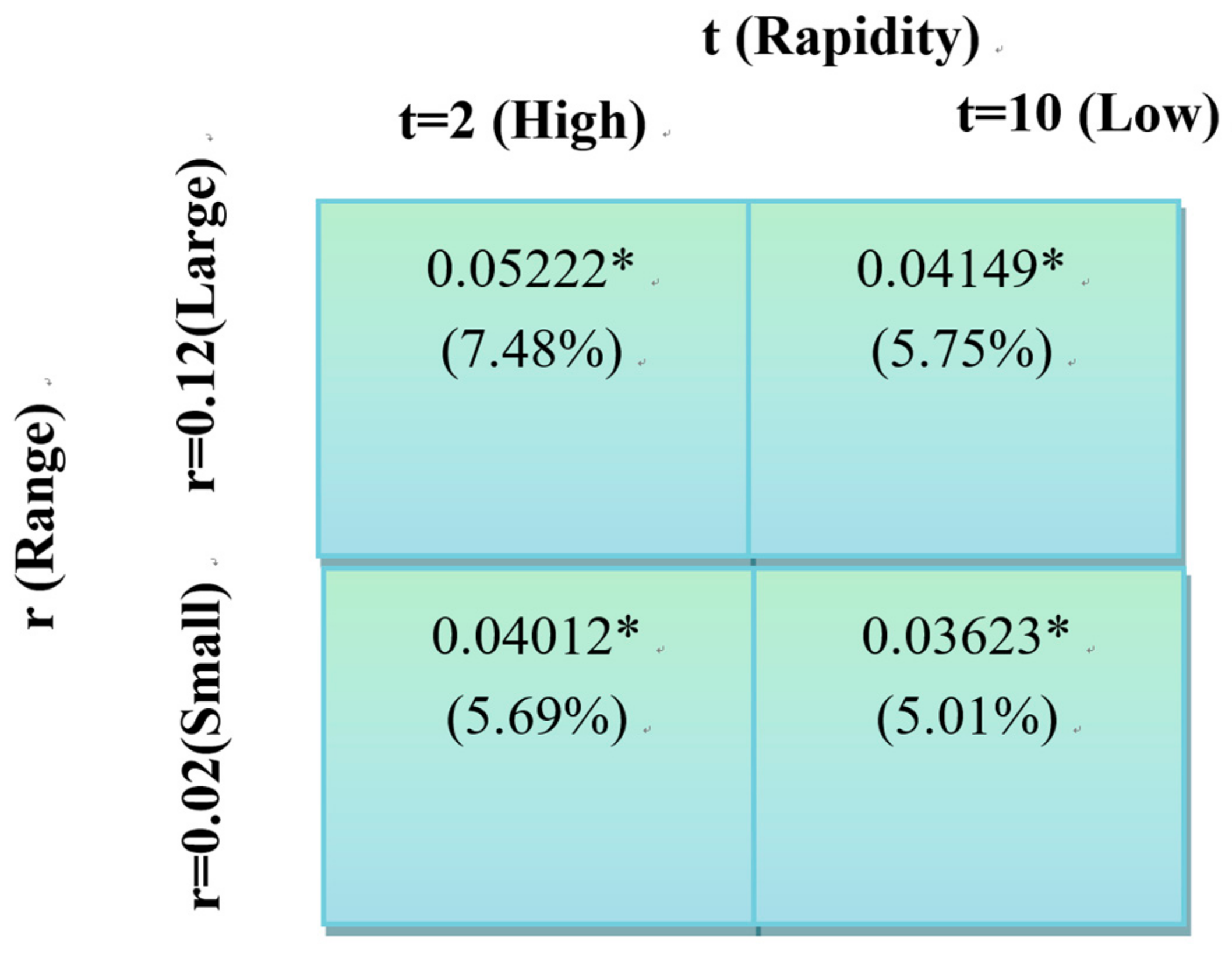
Figure 6.
Mean differences between high and medium (K = 5). Note: each result in Figure 6 is an average over 30 landscapes. * The mean difference is significant at the 0.05 level.
Figure 6.
Mean differences between high and medium (K = 5). Note: each result in Figure 6 is an average over 30 landscapes. * The mean difference is significant at the 0.05 level.


Table 1.
Mean difference in stable landscapes.
| K | MD between Medium and Low | MD between High and Medium |
|---|---|---|
| K = 1 | 0.01043 (1.47%) | 0.00103 (0.15%) |
| K = 3 | 0.03632 * (5.15%) | 0.00236 (0.32%) |
| K = 5 | 0.04371 * (6.06%) | 0.00351 (0.46%) |
| K = 7 | 0.04840 * (6.86%) | 0.00381 (0.51%) |
| K = 9 | 0.05661 * (8.14%) | 0.01217 * (1.62%) |
| K = 11 | 0.06696 * (9.70%) | 0.02249 * (2.93%) |
Each result in Table 1 is an average over 30 landscapes. * The mean difference is significant at the 0.05 level.
Table 2.
Mean differences in dynamic landscapes (t = 2, r = 0.12).
| K | MD between Medium and Low | MD between High and Medium |
|---|---|---|
| K = 1 | 0.02107 * (3.08%) | 0.00358 (0.51%) |
| K = 3 | 0.04135 * (5.99%) | 0.00850 (1.16%) |
| K = 5 | 0.05222 * (7.48%) | 0.01558 * (2.08%) |
| K = 7 | 0.05870 * (8.49%) | 0.01871 * (2.49%) |
| K = 9 | 0.06124 * (8.88%) | 0.02718 * (3.62%) |
| K = 11 | 0.06943 * (10.4%) | 0.03673 * (4.99%) |
Each result in Table 2 is an average over 30 landscapes. * The mean difference is significant at the 0.05 level.
© 2019 by the authors. Licensee MDPI, Basel, Switzerland. This article is an open access article distributed under the terms and conditions of the Creative Commons Attribution (CC BY) license (http://creativecommons.org/licenses/by/4.0/).
Share and Cite
MDPI and ACS Style
Li, F.; Chen, J.; Ying, Y. Innovation Search Scope, Technological Complexity, and Environmental Turbulence: A N-K Simulation. Sustainability 2019, 11, 4279. https://doi.org/10.3390/su11164279
AMA Style
Li F, Chen J, Ying Y. Innovation Search Scope, Technological Complexity, and Environmental Turbulence: A N-K Simulation. Sustainability. 2019; 11(16):4279. https://doi.org/10.3390/su11164279
Chicago/Turabian StyleLi, Fei, Jin Chen, and Ying Ying. 2019. "Innovation Search Scope, Technological Complexity, and Environmental Turbulence: A N-K Simulation" Sustainability 11, no. 16: 4279. https://doi.org/10.3390/su11164279
Note that from the first issue of 2016, this journal uses article numbers instead of page numbers. See further details here.