Acquiring and Geo-Visualizing Aviation Carbon Footprint among Urban Agglomerations in China

Abstract

This paper had two main purposes. One was to estimate annual total aviation CO₂ emissions from/among all key urban agglomerations (UAs) in China and its changes patterns from 2007 to 2014. The second one was to visualize the aviation carbon footprints among the UAs by using a chord diagram plot. This study also used Kaya identity to decompose the contribution of potential driving forces behind the aviation CO₂ emissions using Kaya identity. Especially, it decomposed factor CO₂/gross domestic product (GDP), which is wildly used in Kaya identity analysis, into factor CO₂/value-added (VA) and factor VA/GDP. Here, VA represents the tourism value added of the corresponding flights. The main results were: (1) The UAs developed a much bigger and stronger carbon network among themselves. (2) There was also an expanding of the flows to less densely populated or less developed UAs. However, the regional disparity increased significantly. (3) Compared with the driving factor of population, the GDP per capita impacted the emission amount more significantly. Our contribution had two folds. First, it advances current knowledge by fulfilling the research gap between transport emissions and UA relationship. Second, it provides a new approach to visualizing the aviation carbon footprints as well as the relationships among UAs.

1. Introduction

Living in an age where urban areas expand rapidly and the interaction between cities grows frequently, urban agglomeration (UA) sustainability has become a hot topic for researchers since 1990s. Within previous studies, the transport sector has gained widely concerns due to it is one of main contributors of UA air pollutions and greenhouse gas (GHG) emissions [1]. It is argued that, to achieve urban sustainability, we need to measure and control the emissions from the transportation sector [2,3]. Policies that encourage transport and urban design integration (driving CO₂ reduction by integrating transport and urban design strategies, 2011), urban land-use regulation [4], transportation shift from higher emission models to lower emission ones (sustainable passenger road transport scenarios to reduce fuel consumption, air pollutants and GHG (greenhouse gas) emissions in the Mexico City metropolitan area), such as to non-motorized transport models or public transport models (Deepty Jain and Geetam Tiwari [5]), or reduce vehicle-miles traveled are typically considered as means to reduce GHG emissions in an urban area (passenger travel CO₂ emissions in US urbanized areas: Multi-sourced data, impacts of influencing factors and policy implications, 2014) [2]. Furthermore, according to the World Conference on Transport Research’s project, the ‘Comparative study on Urban Transport and the Environment’, urban low-carbon transport measures could be divided into two categories—‘Strategies’ and ‘Instruments’ (Nagamura et al. [6]), and Nakamura and Hayashi [7] summarized these strategies into three components: Avoid, shift and improve, based on the so-called avoid–shift–improve (ASI) framework. These previous studies solely focused on the emissions of a single urban area or UA [8]. To the best of our knowledge, there have been relatively few studies exploring transport emissions and interrelations among UAs.

Yet, it is difficult to assess transportation emissions among UAs due to the complexity of traffic modes and volume. Alternatively, it is a possible approach to address this issue by estimating aviation CO₂ emissions between UAs based on methods provided by the European Environment Agency (EEA), EUROCONTROL or Corinair. Such as Alonso et al. [9], calculated the aviation CO₂ emissions distribution among EU countries; Wu et al. [10] compared the CO₂ emissions of China’s domestic aviation market and found that the airports located in the Beijing–Tianjin–Hebei, the Yangtze River Delta and the Pearl River Delta UAs totally accounted for half of the overall annual emissions. However, the emissions were generally emitted by flights bound to other UAs or regions probably due to two reasons: (1) The major cities in each UA are well connected by surface transport modes and the surface transport modes have replaced inter-region flights; and (2) these UAs have not yet built interconnection transportation networks among themselves or to other UAs. This study quantitatively supports decision making in developing a low-carbon aviation industry in China but did not focus on UAs relationships or carbon footprints.

Based on the above background, this paper has three study purposes. (1) To investigate the aviation CO₂ emissions in terms of UAs in China; (2) to visualize aviation carbon footprints among the UAs and (3) to estimate the impacts of regional disparities on the carbon footprints and its directions. This study takes all key UAs as study areas, and the study period is from 2007 to 2014. Primarily, we develop two aviation datasets utilizing big data mining technology, then calculate the annual emission quantities based on the EEA method. Moreover, based on the calculation result, we use the chord diagram plot to visualize the emissions footprints among the UAs and cities. Furthermore, we use Kaya identity to decompose the contribution of key driving forces behind the emissions, as well as to estimate the direction of carbon footprints. Our contribution has two folds. First, it advances current knowledge by fulfilling the research gap between transport emissions and UA relationship. Second, it provides a new approach to visualizing the aviation carbon footprints as well as the relationships among UAs.

2. UAs in China

According to China’s ‘13th Five-Year Plan’ issued by the National Development and Reform Commission of China, there are 19 key urban agglomerations in China (http://www.ndrc.gov.cn/zcfbghwb/). These are the Beibu Gulf (BG), Beijing–Tianjin–Hebei (BT), Chengdu–Chongqing (CC), Central Guizhou (CG), Central Southern of Liaoning (CL), Central Plains (CP), Central Shaanxi Plain (CS), Central Yunnan (CY), Hohhot–Baotou–Ordos–Yulin (HB), Harbin–Changchun (HC), the areas along the Huanghe River in Ningxia (HN), the Jinzhong regions (JR), Lanzhou–Xining (LX), the Middle-reaches of the Yangtze River (MY), the northern slopes of the Tianshan Mountains (NT), the Pearl River Delta (PR), the Shandong Peninsula (SP), West Coast of the Straits (WC) and the Yangtze River Delta (YR).

These UAs are the most developed areas in China. It is expected that these UAs will totally account for 74% of the country’s urban population by the end of 2020 (NDRC, 2019) [11]. Using the data derived from the 1:1 million basic geographic databases of the National Basic Geographic Information Center of China, we developed Figure 1 to show the geographical location of all UAs, where green blocks refer to UA boundaries, grey ones are provincial boundaries and red circles present major cities. It could be observed that (1) the UAs were located separately, albeit some of them even crossed the provincial boundaries; (2) it included most of the provincial capital and municipality directly under the Central Government (the biggest red circle).

On the other side, there are sharp and growing regional variations among the UAs regarding the gross domestic product (GDP), per capita income, transportation infrastructure or natural resources. Such as the top five UAs (BT, PR, YR, CC and MY) totally contribute to 55% of the country’s GDP; while the rest of the 14 UAs only contributed to 45% of the GDP.

Table 1. Population number of each urban agglomeration (in million).

	Urban Agglomeration	2007	2014	Chang Rate (%)
1	Beibu Gulf (BG)	16.74	17.86	6.69%
2	Beijing–Tianjin–Hebei (BT)	54.97	72.34	31.60%
3	Chengdu–Chongqing (CC)	68.75	69.04	0.43%
4	Central Guizhou (CG)	33.17	28.40	−14.37%
5	Central Southern of Liaoning (CL)	18.81	19.13	1.69%
6	Central Plains (CP)	42.49	42.83	0.80%
7	Central Shaanxi Plain (CS)	10.16	10.38	2.18%
8	Central Yunnan (CY)	5.18	5.51	6.34%
9	Hohhot–Baotou–Ordos–Yulin (HB)	9.58	10.60	10.61%
10	Harbin–Changchun (HC)	30.62	30.49	−0.43%
11	The Areas Along the Huanghe River in Ningxia (HN)	2.55	3.09	21.39%
12	The Jinzhong Regions (JR)	7.13	7.51	5.35%
13	Lanzhou–Xining (LX)	8.64	9.08	5.04%
14	The Middle Reaches of The Yangtze River (MY)	54.49	56.21	3.14%
15	The Northern Slopes of the Tianshan Mountains (NT)	2.47	2.97	19.96%
16	The Pearl River Delta (PR)	11.93	14.01	17.45%
17	The Shandong Peninsula (SP)	28.85	34.71	20.34%
18	West Coast of the Straits (WC)	49.46	52.88	6.90%
19	The Yangtze River Delta (YR)	79.99	94.66	18.34%

Source: National Bureau of Statistics of China, percentages are author calculated.

lists the population of each UA. It indicates a huge population disparity among the UAs in terms of total amount (from 72.34 million of BT to 2.97 million of NT) and change rate. From a geographical perspective, Liu et al. [12] founded that the UAs with the greatest values of factors comprehensive aggregating ability were mainly centralized in the prosperous eastern corridor of China, while the UAs located in the western China had the lowest comprehensive ability. Especially, there is a declining gradient pattern from east to west, and this declining pattern is consistent with the regional differences of GDP and population distributions.

Many researchers have explored the environmental issues related to Chinese UAs over the last decade. However, the previous studies published in English journals almost took a single UA as the study area, especially, Beijing–Tianjin–Hebei (e.g., Hao et al. [13]; Zhang et al. [14]; Li et al. [15]), the Yangtze River Delta urban agglomeration (Guo et al. [16]; Zhen et al. [17]; Zhang et al. [18]; Liu et al. [19]) or the Pearl River Delta urban agglomeration (e.g., Wang et al. [20]; Ye et al. [21]; Lu et al. [22]). Alternatively, few attentions have been paid to multiple agglomerations nor the interactions among them. Meanwhile, those studies mainly addressed issues related to landscape metrics, urban size, energy flow, ecological networks or urban metabolism. Whilst the estimation of transportation emissions is a quantified way to reach the UA sustainability goal, few researchers have paid attentions to this issue.

It is worth noticing that recent papers published by ‘Sustainability’ addressed some new topics and expanded the study areas. Such as Liu et al. [10] estimated the spatial differences of all China’s key UAs in terms of factors aggregating ability. It is one of the important issues to study UA sustainability on a national scale. China is facing serious environmental problems caused by regional socio-economic development, physical geography, industrial layout and low-carbon city policy disparities (Huang and He [23]; Liu and Bo [24]). Regarding CO₂ emissions, some researchers have studied the regional inequity among the Chinese provinces. For example, Dong and Liang [25] found a significant emission leakage among 30 Chinese provinces and Luo et al. [26] analyzed the regional disparity of freight CO₂ emissions in China’s three regions, arguing that the economic structure is the key factor leading to the disparity. Therefore, this study estimates aviation transportation emissions among all key UAs and its cities, with a focus on regional disparities.

3. Methods and Data Sources

3.1. CO₂ Emissions Calculation

The European Environment Agency (EEA, 2013a, b) [27,28] provides a standard method to estimate CO₂ emissions in terms of seats, routes or airlines. Other calculation methods—for example EUROCONTROL or Corinair—are also used by researchers to evaluate aviation emissions. However, these methods are based on the indicator available seat kilometers (ASK; Alonso et al. [9]; Scotti and Volta [29]; Kousoulidou and Lonza [30]). This study used the EEA emissions calculation method for two reasons: First, ASK is mainly used to measure an airline’s passenger carrying capacity; therefore, CO₂/ASK is normally used to express an airlines’ emission level such as emission intensity. Second, this study aimed to determine the regional disparity rather than airlines’ performance.

According to the EEA method, the total emissions ($E_{C{O}_2}$) are the sum of emissions produced during an aircraft landing and take-off cycle ($LT{O}_{C{O}_2}$) as well as during the aircraft cruising period ($C{R}_{C{O}_2}$), see Equation (1).

$$E_{C{O}_2}=LT{O}_{C{O}_2}+C{R}_{C{O}_2}={\sum }_i\left[\left(LT{O}_{C{O}_2,i,j}+C{R}_{C{O}_2,i,j,d}\right)·w\right],$$

(1)

where the emissions of each flight i during the landing and take-off cycle ($LT{O}_{C{O}_2,i,j}$) is a fixed value due to the aircraft type j. The emissions during the cruising period ($C{R}_{C{O}_2,i,j,d}$) is a flexible value due to aircraft type j and travel distance d. By multiplying each flight’s emissions with its annual frequency w and calculating the emissions of each flight i, the formula obtains the total emissions from all airlines. We adjusted several regional aircraft types, which are not recorded in standard forms, into standard types according to the EEA guidebook.

Two sets of air traffic data were used to calculate the emissions. The first was the air traffic dataset, which included aircraft type, route (origin-to-destination, OD) and seat supplement in the years 2007 and 2014. The source of this data was China’s domestic air passenger timetable published by the Civil Aviation Administration of China (CAAC). The second dataset—to determine the flown distance of each route—was retrieved from the China Travel Sky reservation system. Specifically, the following aviation data were retrieved:

-

Passenger airports of the 19 UAs and all their routes (on city-pair level) within/between the UAs. In more detail, information concerning flight routes, flight frequency per route, aircraft type and passenger seats available per flight was obtained.

-

Actual flown distance for each route. Flying distance is a key indicator to calculate aircraft emissions during the cruising period. Some researchers have calculated aircraft emissions during cruising periods but measured the route distance by using the airports’ geographical coordinates (Alonso et al. [9]) or great circle distances (Scotti and Volta [29]). To calculate emissions more precisely, we mined the flown distance of each route from Chinese Travel Sky reservation system.

-

Since many major aircrafts provide flexible seating, we used the number of seats as illustrated in

Table 2. Number of seats of major aircrafts.

Airbus Family		Boeing Family
Aircraft Type	Estimated Number of Seats Per Flight	Aircraft Type	Estimated Number of Seats Per Flight
A320	158	B737 (300, 800)	128, 159
A330 (200, 300)	237, 301	B757 (200)	200
A340-300	255	B767 (300ER)	233
A319	128	B747 (Combi)	280
A321	185	B777 (300ER)	311

Source: Relative airlines’ website.

. Meanwhile, the seating provided by major aircraft types was adjusted according to an average.

3.2. Carbon Footprints Visualization

This visualization reveals UA relationships by depicting the aviation carbon footprints between UAs and cities. Carbon footprint generally refers to the amount of CO₂-equivalent emissions caused by both direct and indirect activities. In this study, however, ‘carbon footprint’ refers to CO₂ emissions emitted directly by flight operations. Generally, researchers input their calculation results into the ArcGIS platform to illustrate or calculate the spatial distributions of footprints between two regions or cities (Dong and Liang [25]; Wu et al. [10]). However, Lenzen et al. [31] evaluated the direct carbon emissions of tourism activities as well as the carbon emitted by producing tourist commodities globally. They also attempted to map the carbon footprints but could not visualize the footprints’ direction precisely.

To visualize the complex UA relationships, we used a chord diagram plot. The chord diagram plot is a useful instrument to investigate bilateral flows by identifying the source, destination, direction and volume. Therefore, a chord diagram plot was used to visualize aviation carbon footprints between UAs and cities with the help of the circlize package in R. The chord diagram plots visually represent the direction and volume of carbon footprints.

3.3. Kaya Identity

Kaya identity is a formula that relates the rates of carbon emission to various parameters such as the population, gross domestic product (GDP) per capita, energy intensity or carbon intensity of the energy supply (Kaya [32]). This study revises the Kaya identity to decompose the contribution of potential driving forces behind aviation CO₂ emissions. Factor CO₂/GDP has been widely used in the Kaya identity analysis. However, it is not straightforward to define the factor CO₂/GDP in our study, due to the GDP being the total value of goods and services produced by each UA, but the CO₂ emissions only refers to the emissions produced by air transportation sector. Therefore, we introduced value-added (VA) as one of the key factors, then decomposed the CO₂/GDP to CO₂/VA and VA/GDP. Here, VA represents the value added of the corresponding flights.

Especially, this study focused on the tourism value added of the corresponding flights in terms of the UA. The linkage between the aviation industry and tourism industry has been a hot topic over the last two decades, in both aviation and tourism research fields (Bojana et al. [33]; Wu et al. [34]; Marco and Alberto [35]). It is generally believed that the aviation industry can bring overall benefits to local economics, and some of these benefits such as the development of the tourism industry, can be directly quantified (Button and Taylor [36]). Thus, using the value-added (VA) approach, Fung et al. [37] measured the benefits that the aviation industry contributed to the Hong Kong economy successfully, and found that the tourism industry contributed to 0.54% of the GDP. Meanwhile, some researches, which study the tourism carbon footprint, began to emphasize the emissions from the air transport sector in recent years (e.g., Sun [38]; Sharp [39]; Lenzen et al. [31]). According to Lenzen et al. [31], the contribution of air travel emissions amounts to 20% of tourism’s global carbon footprint, while air travel would come out as the dominant emissions component in some situations. Furthermore, some evidences indicate that air transportation emission reduction projects could impact tourism industry. Chen et al. [40] adopted the input–output method (I–O) to measure the economic contribution of the air transportation energy conservation and emission reduction (ECER) projects in China. Based on the 139-sectors I–O tables published by the local Bureau of Statistics of Beijing, Tianjin and Hebei, Chen et al. [40] calculated the value-added coefficient, the complete consumption coefficient and the complete partition coefficient of the Beijing–Tianjin–Hebei region. Their calculation results indicate, in terms of the value-added coefficient, the cultural, art and entertainment and activities sector ranked 7th; other tourism related sectors (such as the accommodations sector, business services sector or sports activities sector) were all the top 20% sectors. Thus, it is reasonable to assume that (1) tourism could present the aviation additional value at a certain degree; and (2) there is a significant relationship between aviation emissions and tourism industry.

To make the work tractable, the study used the number of the national high-class tourism scenic area (5A and 4A level only) owned by each UA as the key indicator to describe the tourism value added of the corresponding flights. This is because the high-class tourism scenic area is a relatively robust and measurable indicator of a UA’s tourism success. China National Tourism Administration (CNTA) started the scenic areas normative and standardized quality rating system in 2007. According to this system, China’s scenic areas can be divided into five levels from AAAAA (5A), AAAA(4A), AAA(3A), AA(2A) and A(1A). Of which, 5A presents the world class tourism quality; 4A presents the national class tourism quality. Both 5A and 4A scenic areas are called high-class level scenic areas. To become a 5A or 4A-scenic area, one should live up to the CNTA inspection items standards such as transportation, tourism safety and capability. Regarding to the transportation, the first requirement is that 5A or 4A scenic areas should be located nearby airports (within two hours transportation). It means that the high-class tourism scenic area is always located near the airports. Alternatively, the number of the tourism scenic area could have a positive relationship with the air transportation sector.

Therefore, we rewrite the original equation to Equation (2).

$$C{O}_2=\frac{C{O}_2}{VA}\times \frac{VA}{GDP}\times \frac{GDP}{P}\times P$$

(2)

In which, $C{O}_2$: The aviation carbon emissions; VA refers to value added of the corresponding flights, which equals the number of high-class tourism scenic areas (5A and 4A level only) owned by each UA in different years; GDP means the total GDP of cities served by airports within each UA and $p$ is the population of these cities. In this way, $\frac{C{O}_2}{VA}$ means emission intensity per VA, $\frac{VA}{GDP}$ means added value per GDP and $\frac{GDP}{P}$ means GDP per capita in terms of UA, which is affluence. Through mathematical transformation, the original equation can be rewritten as Equation (3).

$$d\left(\ln C{O}_2\right)=d\left(\ln \frac{C{O}_2}{VA}\right)+d\left(\ln \frac{VA}{GDP}\right)+d\left(\ln \frac{GDP}{P}\right)+d\left(\ln P\right).$$

(3)

Based on Equation (3), with a small change in the variables on the right side of the formula, the sum of the rate of change was considered to be approximately equal to the rate of change of CO₂ emissions during the corresponding period. Therefore, we could determine to what extent these factors had an influence on aviation carbon emissions in terms of UA.

The population and GDP datasets were assessed from the China Urban Statistical Year Books. Normally, we selected the data in terms of city, then added the data together according to UA. The datasets of national high-class tourism scenic areas were assessed from CNTA.

4. Results

4.1. Changes in Total CO₂ Emissions Produced by the UAs

The calculation results show that the total annual CO₂ emissions produced by all 19 UAs (including the emission produced by domestic flights between UAs, between UA and non-UA areas and between cities within a UA) increased from 24.6 million tons in 2007 to 44 million tons in 2014. The average increase rate was 78.72%.

Table 3. Changes in the total emission amounts per UA, 2007 vs. 2014.

UA	2007		2014		Changes from 2007 to 2014
	Emissions Amount	Share among All UAs	Emissions Amount	Share among All UAs	Emissions Amount	Change Rate by Percentage	Changes Rate by the Share
BC	850	3.45%	1475	3.35%	625	73.49%	−0.10%
BT	3857	15.67%	6571	14.94%	2714	70.37%	−0.73%
CC	2386	9.69%	3721	8.46%	1335	55.96%	−1.23%
CG	343	1.39%	802	1.82%	459	133.75%	0.43%
CL	821	3.34%	1268	2.88%	447	54.43%	−0.45%
CP	495	2.01%	1214	2.76%	719	145.43%	0.75%
CS	805	3.27%	1389	3.16%	583	72.46%	−0.11%
CY	1060	4.31%	1719	3.91%	659	62.16%	−0.40%
HB	160	0.65%	590	1.34%	430	269.07%	0.69%
HC	637	2.59%	1366	3.11%	730	114.63%	0.52%
HN	80	0.32%	294	0.67%	214	267.86%	0.34%
JR	262	1.06%	497	1.13%	235	89.63%	0.07%
LX	372	1.51%	610	1.39%	239	64.19%	−0.12%
MY	1334	5.42%	3370	7.66%	2036	152.60%	2.24%
NT	800	3.25%	1572	3.57%	772	96.57%	0.32%
PR	3737	15.18%	5644	12.83%	1907	51.04%	−2.35%
SP	888	3.61%	1463	3.32%	574	64.67%	−0.28%
WC	1344	5.46%	2439	5.54%	1095	81.45%	0.08%
YR	4389	17.83%	7995	18.17%	3606	82.16%	0.34%
Total	24,619	100.00%	43,998	100.00%	19,379	78.72%	0.00%

demonstrates the change of emission amount in terms of UA. According to the amount of emissions produced, YR, BT and PR were the top three UAs in both 2007 and 2014. Furthermore, an obvious rising trend of emissions in the middle and western parts of China was observable, such as in CC, WC, MY and CY.

Concerning the change rate by amount, HB saw the fastest increase rate (269.07%), followed by HN (267.86%) and MY (152.60%). Both oHB and HN are located along the Silk Road, an area that has been experiencing a rapid increase in population and air transportation under the One Belt One Road Initiative. MY was shown to have the largest emission share growth among the UAs within the Yangtze River Economic Belt. This could be because this UA had experienced rapid economic growth and airport construction such as8 airports were newly opened during the study period.

In terms of the change rate by share, half of the UAs emission shares declined, especially PR shows the maximum decline share ratio of −2.35% and BT decreased by −0.73%. This was probably because fully connected land transport networks as well as HSR (high speed rail) networks were constructed within the UA BT and other UAs. This means that travelers may prefer to take land transportation instead of air transport. It may also be because we did not include Hong Kong International Airport in our calculation, which decreased PR’s share significantly.

4.2. Changes in the Emissions among UAs

The results indicate that CO₂ emissions produced by the domestic flights between UAs increased from 24.16 to 37.28 million tons. The increase rate was 54.3%, which was nearly 25% lower than the increase of total emissions produced by the UAs (78.72%). Considering the share of emissions produced by flights between UA and non-UA areas increased from 1.87% to 15.28%, we could see that the UAs had a much stronger carbon network among themselves, and there was an increase in carbon flow between UAs and non-UA areas.

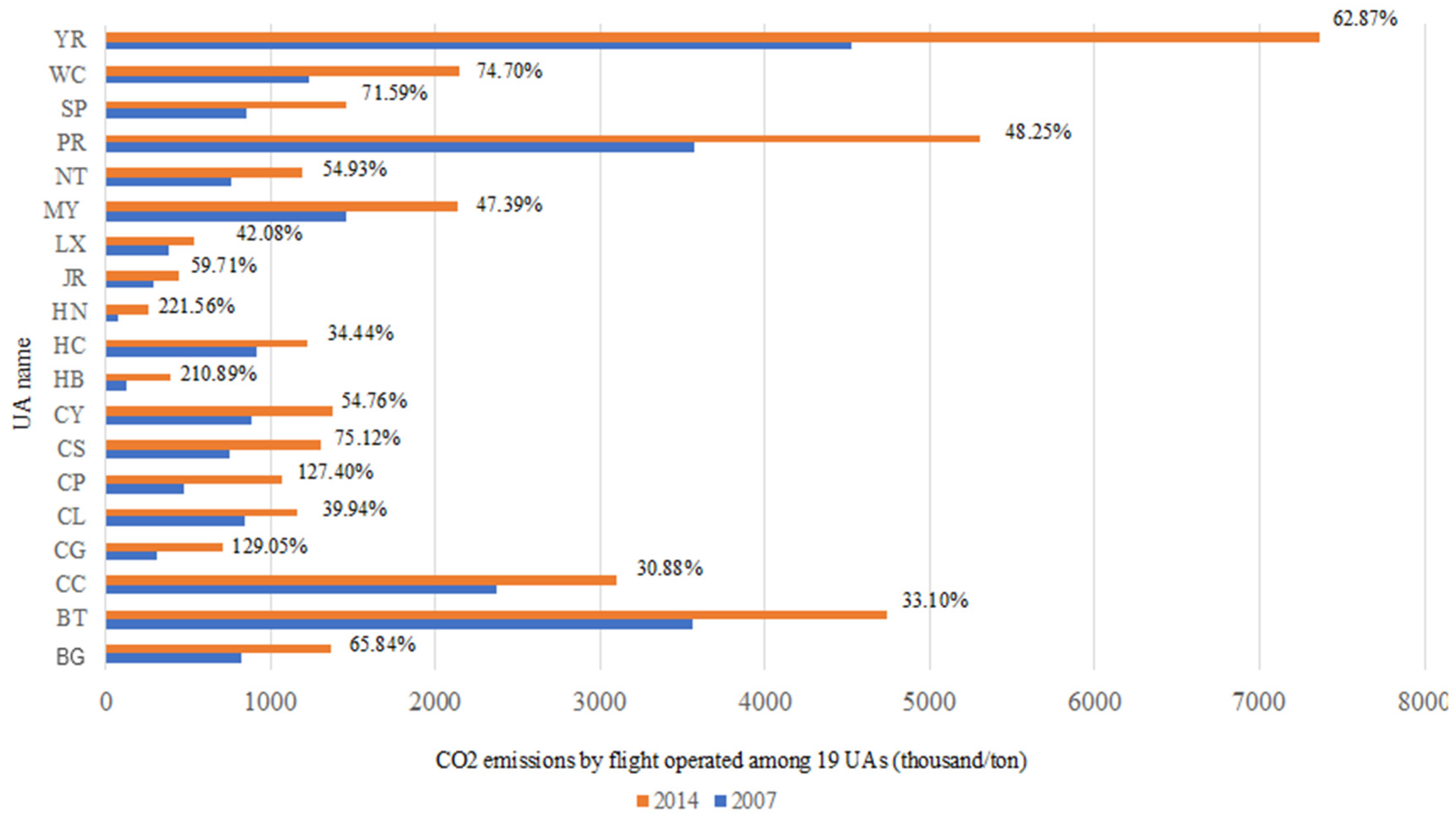
Figure 2 shows the changes in the CO₂ emissions in terms of the UA. It indicates that there was an increase in carbon flows to less densely populated or less developed UAs. According to the emission amount, the top five UAs were YR, BT, PR, CC and MY. On other side, the increase rate of some UAs, which were located in less densely populated or remote areas, such as HN, HB, CP, CS and WC, excessed 100%. A further data analysis shows that, based on the emission amount, the total share of YR, BT, PR, CC and MY decreased about 3.3%, but the share for HN, HB, CP, CS and WC increased by 2.9%. Looking at these changes, we could see the following change patterns.

Based on a UA-pairs analysis, we also found some interesting patterns.

Table 4. Change in the CO₂ amount based on the UA-pairs.

Emission Amount	No. of UA-Pairs in 2007	No. of UA-Pairs in 2014	Changes
Over 1 million ton	3	7	4
0.5–1 million ton	7	10	3
0.1–0.5 million ton	51	65	14
Less than 0.1 million ton	86	77	−9
Total	147	159	12

shows, from 2007 to 2014, the number of UA-pairs increased from 147 to 152. Of which, the number of UA-pairs produced more than one million tons in emissions increased from 3 to 7, the number of UA-pairs that produced 0.5–1 million tons increased by three, and the UA-pairs produced 0.1–0.5 million tons increased from 51 to 65. Alternatively, the UA-pairs that produced less than 0.1 million tons declined sharply.

Table 5. Changes in routes and average emissions by route (thousand tons).

	In 2007		In 2014		Changes from 2007 to 2014
	Number of Routes	Emissions Per Route	Number of Routes	Emissions Per Route	Number of Routes	Emissions Per Route
BC	60	13.61	97	14.35	37	0.74
BT	116	30.36	178	33.03	62	2.67
CC	106	24.64	154	20.21	48	−4.42
CG	29	10.63	75	9.94	46	−0.69
CL	69	11.94	91	12.95	22	1.01
CP	54	8.49	108	10.00	54	1.51
CS	51	14.37	62	21.11	11	6.74
CY	35	25.16	54	25.72	19	0.56
HB	31	4.11	74	6.63	43	2.52
HC	59	10.46	83	14.54	24	4.07
HN	12	7.25	31	9.13	19	1.88
JR	31	9.04	45	10.13	14	1.09
LX	33	10.36	57	10.02	24	−0.34
MY	129	11.16	175	12.70	46	1.54
NT	22	33.46	28	41.87	6	8.41
PR	122	29.15	166	34.17	44	5.01
SP	90	9.32	116	12.44	26	3.13
WC	111	10.88	158	14.31	47	3.44
YR	217	20.33	325	22.85	108	2.52
Total	1377	17.28	2077	18.92	700	1.63

indicates that the number of air routes among the UAs increased from 1377 to 2077, as well as and the average emissions produced by each route increased by 1.63 million tons. It reveals an increase of disparities among the UAs according to the routes and average emission amounts but could not show UA emission relationships exactly.

4.3. Carbon Footprint Visualization

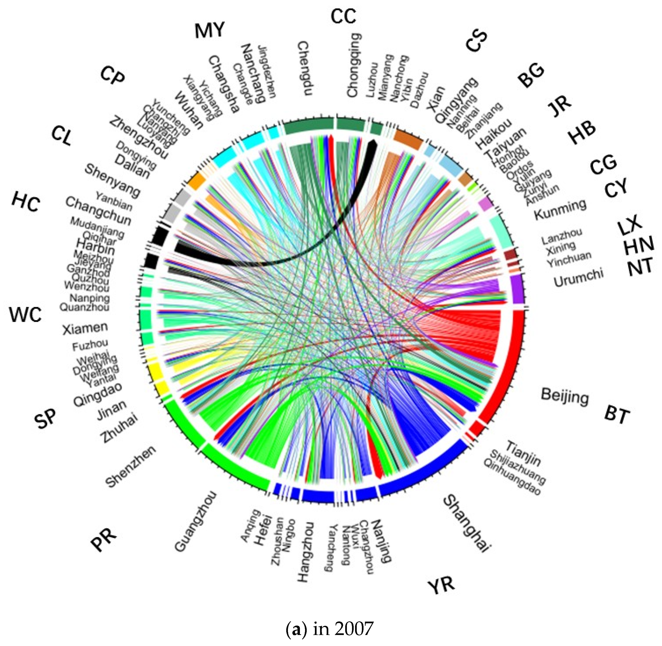
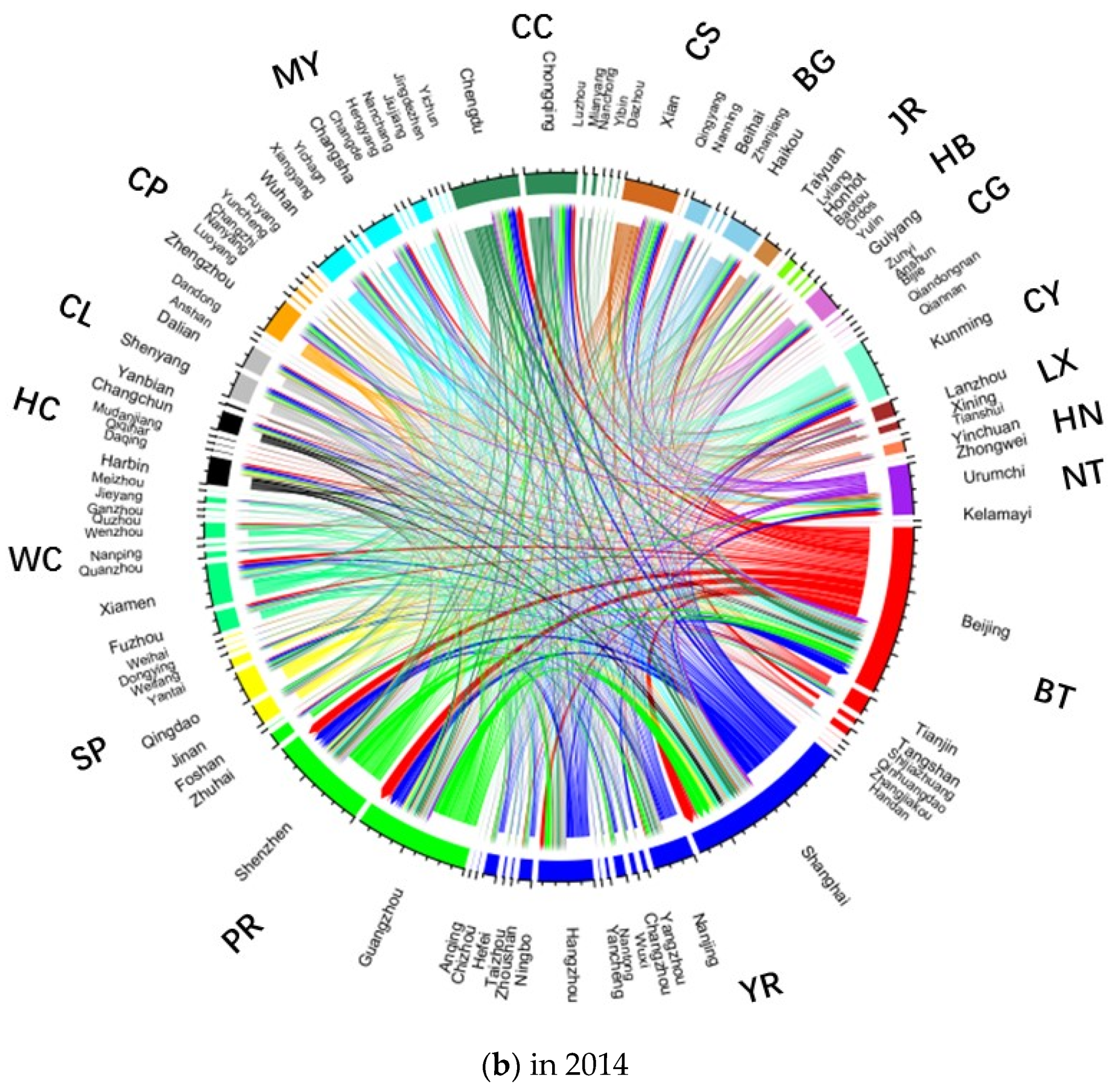
In this section, we used the chord diagram plot to visualize the carbon footprint among the UAs and its change patterns (Figure 3). Yes, we could develop more extensive tables to show the UA relationships according to the emission amount. However, these tables will include the information of more than thousands of routes, making them too big to include in an academic paper. Compared with the traditional tables or figures, this new method could depict the carbon footprints accurately, clearly and scientifically.

In Figure 3, different colors represent different UAs, such as the red is BT, the blue is YR and so forth. The width of lines portrays the emissions amount between the two cities and the arrow point shows the direction of the flight that relates to the direction of the carbon footprint. It could be observed, in both 2007 and 2014, BT, PR and YR showed the largest carbon footprints concerning the radiation range. This was reflected by the UA-pairs reaching the one-million-ton level in 2014 being PR–YR, BT–YR, BT–PR, CC–YR, CC–PR, CC–YR and YR–WC. It was also reflected by the fact that the emissions produced by flights between PR–YR increased nearly 66%, from 2.04 million tons in 2007 to 3.38 million tons in 2014.

Figure 3 also displays the carbon flows in terms of cities. According to the emission amount, the cities can be classified into three groups: Core cities, semi-core cities and periphery cities. In both years, Beijing and Shanghai ranked as core cities, followed by Guangzhou and Shenzhen, which are both located in and have become new core-cities. Chengdu, Kunming and Urumqi are traditional semi-core cities. In 2014, Hangzhou, Xiamen, Nanjing, Xi’an and Chongqing started changing to semi-core cities. From a geographical perspective, the core cities and semi-core cities form a circle, while the periphery cities are located almost within the circle.

4.4. Driving Factors

This section used Kaya identity to evaluate the impact of key factors on aviation carbon emissions.

Table 6. The impact of aviation carbon emission factors of 19 UAs.

	UA	$\mathit{d}\left(\mathbf{ln}\mathit{C}{\mathit{O}}_2\right)$	$\mathit{d}(\mathbf{ln}\frac{\mathit{C}{\mathit{O}}_2}{\mathit{V}\mathit{A}})$	$\mathit{d}(\mathbf{ln}\frac{\mathit{V}\mathit{A}}{\mathit{G}\mathit{D}\mathit{P}})$	$\mathit{d}(\mathbf{ln}\frac{\mathit{G}\mathit{D}\mathit{P}}{\mathit{P}})$	$\mathit{d}\left(\mathbf{ln}\mathit{P}\right)$
1.	BG	73.49%	73.49%	−64.66%	165.21%	6.69%
2.	BT	70.37%	78.78%	−59.33%	78.04%	31.60%
3.	CC	55.96%	65.32%	−68.06%	194.09%	0.43%
4.	CG	133.75%	33.57%	−49.53%	304.92%	−14.37%
5.	CL	54.43%	39.49%	−50.22%	118.72%	1.69%
6.	CP	145.43%	218.15%	−65.83%	123.97%	0.80%
7.	CS	72.46%	60.14%	−65.66%	206.95%	2.18%
8.	CY	62.16%	41.89%	−56.75%	148.52%	6.34%
9.	HB	269.07%	269.07%	−69.34%	194.91%	10.61%
10.	HC	114.63%	86.63%	−51.32%	137.24%	−0.43%
11.	HN	267.86%	341.44%	−75.22%	177.08%	21.39%
12.	JR	89.63%	−100.00%	−100.00%	96.45%	5.35%
13.	LX	64.19%	49.27%	−60.75%	166.84%	5.04%
14.	MY	152.60%	152.60%	−69.03%	213.09%	3.14%
15.	NT	96.57%	411.07%	−84.48%	106.57%	19.96%
16.	PR	51.04%	57.33%	−58.14%	95.28%	17.45%
17.	SP	64.67%	96.34%	−61.29%	80.05%	20.34%
18.	WC	81.45%	88.17%	−55.70%	103.61%	6.90%
19.	YR	82.16%	121.05%	−64.00%	93.44%	18.34%
	Average	105.36%	114.94%	−64.70%	147.63%	8.60%

is the calculation results. Here, $d\left(\ln C{O}_2\right)$ refers to the change rate of aviation carbon emission, $d(\ln \frac{C{O}_2}{VA})$ refers to the emission intensity factor, $d(\ln \frac{VA}{GDP})$ refers to the added value factor, $d(\ln \frac{GDP}{P})$ refers to affluence factor and $d\left(\ln P\right)$ is the population factor. Meanwhile, each value represents the impacting ratio of the factors on the total CO₂ change rate, such as a positive value means higher CO₂ emissions and a negative value means lower CO₂ emissions.

Figure 4 complements Table 6 to clarify the results further. It shows, (1) each UA presented a positive and negative offset; (2) all of the factors demonstrated positive effects, excepting the added value factor and (3) the 19 UAs could be divided into two groups according to the differences in the results. The first group was UAs that only showed one negative factor, including BG, BT, CC, CL, CP, CS, CY, HB, HN, LX, MY, NT, PR, SP, WC and YR. The second group was UAs that showed two negative factors, including CG, HC and JR.

Generally, the results show that, in most of the UAs, the rapid growth of resident’s disposable income was strongly consistent with the increase in CO₂ emissions; the population factor also showed some positive impacts but only had a limited influence. Regarding to CG and HC, we could see that the population factor showed positive impacts. One of the possible explanations should be that those two UAs had two core cities (i.e., Chengdu and Chongqing in CG, Harbin and Changchun in HC), and the core cities were connected by newly established high-speed railways (HSR), which decreased air traffic within UAs. The situation of JR was very special. It was possibly due to the number of high-level scenic spots located within JR dropped from 2 to 0 over the studying period, which made the calculation results lose significance.

Meanwhile, based on Equation (2), we conducted a regression analysis to detect the different influence levels that all Kaya factors have on the CO₂ emissions. Firstly, an F-test was conducted to check the feasibility of this regression model, based on the changed volume of independent variables (emission intensity per VA, tourism value per GDP, GDP per capita and population) and dependent variable (aviation carbon emission).

Table 7. ANOVA test results ^a of the regression model availability.

Model	Sum of Square	Df	Mean Square	F	Sig.
Regression b	6.90 × 1018	4	1.73 × 1018	29.806	0.000.
Residual	4.63 × 1018	80	5.79 × 1016
Total	1.15 × 1019	84

^a: Predictor (constant): Difference in carbon intensity per VA, difference in tourism value per GDP, difference in GDP per capita and difference in population. ^b: R-squared = 0.598, adjusted R-square = 0.578. ^c: Dependent variable: Difference in CO₂ emissions.

presents the ANOVA results, which show those predictors are significantly related to the dependent variable (at the significant level of 0.05). Besides, the R-square and the adjusted R-square here were 0.598 and 0.578 respectively, though being a medium degree of interpretation, the gap between those two values was small, thus it could still be acceptable. The overall results indicate that this regression model was able to explain to what extent does those four predictors had an impact on the CO₂ emissions.

Table 8. Regression coefficient ^a.

Unstandardized Coefficient				Standardized Coefficient		Collinear Statistics
Model	B	Standard Error	Beta	t	Sig.	Tolerance	VIF
(constant)	−2.14 × 107	5.17 × 107		−0.415	0.680
Carbon intensity per VA	1.12 × 100	5.48 × 10−1	0.158	2.050	0.044	0.842	1.187
Tourism value per GDP	−1.34 × 1010	1.02 × 1010	−0.097	−1.315	0.192	0.918	1.089
GDP per capita	1.62 × 107	6.35 × 106	0.185	2.552	0.013	0.952	1.050
Population	1.53 × 106	1.66 × 105	0.705	9.198	0.000	0.854	1.171

^a: Dependent variable: Difference in CO₂ emissions.

shows the regression results, from which, we could observe that (1) the population factor was the most influential factor that boosted the CO₂ emissions, followed by the affluence factor and the added value factor had the least impact. It means, the increase of population and residents’ disposable income could give rise to the CO₂ emissions, while the increase of scenic spots just slightly led to the growth of CO₂ emissions. (2) At a significant level of 0.05, the changes in population, affluence and carbon emission intensity factors were positively related to the change in CO₂ emissions, which means that when anyone of those factors grows, the CO₂ emissions will go up accordingly.

Table 9. Collinear diagnosis result ^a.

			Variance Proportion
Dimension	Eigenvalue	Condition Index	(Constant)	Carbon Intensity Per VA	Tourism Value Per GDP	GDP Per Capita	Population
1	2.888	1.000	0.03	0.04	0.03	0.03	0.02
2	0.950	1.744	0.01	0.05	0.03	0.06	0.56
3	0.549	2.293	0.00	0.10	0.28	0.41	0.06
4	0.446	2.545	0.04	0.80	0.14	0.03	0.24
5	0.167	4.160	0.92	0.01	0.51	0.47	0.11

^a: Dependent variable: Difference in CO₂ emissions.

presents the collinear diagnosis result. Combining the collinear statistics in Table 8, we could see that (1) all the VIF values and condition indices were less than 10, (2) all the eigenvalues were not zero and (2) only few values in the correlation coefficient matrix were close to 1. Here, VIF refers to variance inflation factor which represents the ratio of the variance between the explanatory variables with collinearity, as well as the variance without collinearity, and the bigger the VIF value is, the more serious collinearities exist. Above results It means that the model was acceptable, for no serious collinearities between the variables was found. Thus, we can see the regression results were reliable.

5. Discussion and Conclusions

Estimation of transportation emissions is a quantified way to reach the UA sustainability goal. In this study, we calculated the CO₂ emissions produced by domestic passenger flights within and among the key UAs in China, in year 2007 and 2014. Based on calculation results, we visualized the aviation carbon footprints by using a chord diagram plot, then, investigated the potential impacts of economic, population and value added by corresponding flights on the carbon footprints in terms of the UA. This study advances current knowledge by fulfilling the research gap between transport emissions and UA relationship, and provides a new approach to visualizing the transportation carbon footprints as well as the relationships among multiple UAs.

Firstly, the annual total CO₂ emissions produced by air flights to and from the UAs (including the domestic flights served the routes between UAs, between UA and non-UA areas and between cities within an individual UA) had increased by nearly 78.9%, from approximately 24.6 million tons in 2007 to 44.0 million tons in 2014. Compared with the annual total CO₂ emissions from China’s domestic air passenger transportation, which increased 73.1%, from 27.5 million tons to 47.6 million tons during the same period (Wu et al. [8]), we could see that the emissions produced by the flight connected with UA increased faster than the country level, and more than 90% of the emissions were produced by the flights served in the UAs.

Secondly, based on the analysis of the emissions produced by the domestic flights between UAs, we found the following change patterns. (1) The UAs had a much bigger and stronger carbon network among themselves, which means that the UAs became more closely connected than before. (2) There was an increase of carbon flows between UAs and non-UA areas as well as an increase in the flows to less densely populated or less developed UAs. (3) There was an increase of disparities among the UAs according to the routes and average emission amounts. Generally, those UAs located in the eastern part of China produced more CO₂ emissions. For example, BT, YR and PR produced more than 40% of the emissions and the core cities—Beijing, Shanghai, Guangzhou and Shenzhen—generated large amounts of aviation carbon emissions and exerted high aviation footprints over the seven years. Conversely, the western UAs tended to have higher growth rate due to China’s Western Development and the One Belt One Road Initiative. An example is the rapid growth of central and western UAs like MY and HB as well as cities like Chengdu and Kunming, which can also not be ignored. (4) The chord diagram plot is an effective tool to visualize the carbon footprint among the UAs and cities, as well as its change patterns.

Thirdly, the Kaya identity results showed that factor GDP per capita and factor population were the top two positively influential factors leading to the substantial increase in the carbon emissions. In most cases, the overall carbon emission intensity functioned as a carbon-reduction factor. According to the results, the 19 UAs could be divided into two groups: The one-negative factor group and the two-negative factors group. This study introduced variable VA to the Kaya identity analysis. Here, the VA presents tourism value added of the corresponding flights and evaluated by the number of national high-class tourism scenic area in terms of UA. The results also indicate that the impact of the tourism VA was not as significant as that of the GDP per capita or population. The results of F-tests (with and without VA) showed that few improvements were achieved by adding factor VA into the regression model, which makes it difficult to explain the exact impacts of the factor VA. The possible reasons should be (1) this study only selects the national high-class tourism scenic areas as the indicator to evaluate the tourism VA due to data limitation; and (2) the local governments were all enthusiastic about building more tourism scenic areas over the last decade.

The policy implications of this result were: (1) To achieve the goal of sustainable UAs and cities, UAs should work together to build interconnection transportation networks among themselves, then to promote the modal shift from air transport to surface models. (2) Strengthening the spatial connection is an important way to break bottlenecks of UAs sustainable development. (3) It is important to consider that only balanced development can lead China’s UAs to the promised sustainable goal. This study decomposed the driving forces of aviation carbon emissions through Kaya identity and introduced a new factor VA. It is acknowledged that we will carry out more researches to evaluate the tourism VA and to improve its significances by including more tourism sectors, such as the cultural, art and entertainment and activities sector, accommodation sector, business services sector and sports activities sector in the future. The impacts of more factors—such as the energy intensity factor or the aircrafts type factor—should also be evaluated in further studies.

References

- Liu, C.; Wang, T. Identifying and mapping local contributions of carbon emissions from urban motor and metro transports: A weighted multiproxy allocating approach. Comput. Environ. Urban. 2017, 64, 132–143. [Google Scholar] [CrossRef]
- Vojnovic, I. Urban sustainability: Research, politics, policy and practice. Cities 2014, 41, S30–S44. [Google Scholar] [CrossRef]
- Currie, P.K.; Musango, J.K.; May, N.D. Urban metabolism: A review with reference to Cape Town. Cities 2017, 70, 91–110. [Google Scholar] [CrossRef]
- Leibowicz, B.D. Effects of urban land-use regulations on greenhouse gas emissions. Cities 2017, 70, 135–152. [Google Scholar] [CrossRef]
- Jain, D.; Tiwari, G. How the present would have looked like? Impact of non-motorized transport and public transport infrastructure on travel behavior, energy consumption and CO2 emissions—Delhi, Pune and Patna. Sustain. Cities Soc. 2016, 22, 1–10. [Google Scholar] [CrossRef]
- Nakamura, H.; Arimura, M.; Kobayashi, Y. Overview of Urban Transport and the Environment. In Urban Transport and the Environment: An International Perspective; Emerald: Bingley, UK, 2004; pp. 99–190. [Google Scholar]
- Nakamura, K.; Hayashi, Y. Strategies and instruments for low-carbon urban transport: An international review on trends and effects. Transp. Policy 2013, 29, 264–274. [Google Scholar] [CrossRef]
- Liu, C.; Wang, T.; Lin, X.; Zhao, R. Allocating and mapping carbon footprint at the township scale by correlating industry sectors to land uses. Geogr. Gev. 2016, 106, 441–464. [Google Scholar] [CrossRef]
- Alonso, G.; Benito, A.; Lonza, L.; Kousoulidou, M. Investigations on the distribution of air transport traffic and CO2 emissions within the European Union. J. Air Transp. Manag. 2014, 36, 85–93. [Google Scholar] [CrossRef]
- Wu, C.; He, X.; Dou, Y. Regional disparity and driving forces of CO2 emissions: Evidence from China’s domestic aviation transport sector. J. Transp. Geogr. 2019, 76, 71–82. [Google Scholar] [CrossRef]
- National Development and Reform Commission. 2017. Available online: http://www.ndrc.gov.cn (accessed on 2 March 2018).
- Liu, C.; Wang, T.; Guo, Q. Factors Aggregating Ability and the Regional Differences among China’s Urban Agglomerations. Sustainability 2018, 10, 4179. [Google Scholar] [CrossRef]
- Hao, Y.; Zhang, M.; Zhang, Y.; Fu, C.; Lu, Z. Multi-scale analysis of the energy metabolic processes in the Beijing–Tianjin–Hebei (Jing-Jin-Ji) urban agglomeration. Ecol. Model. 2018, 369, 66–76. [Google Scholar] [CrossRef]
- Zhang, Y.; Zheng, H.; Yang, Z.; Li, Y.; Liu, G.; Su, M.; Yin, X. Urban energy flow processes in the Beijing–Tianjin–Hebei (Jing-Jin-Ji) urban agglomeration: Combining multi-regional input–output tables with ecological network analysis. J. Clean. Prod. 2016, 114, 243–256. [Google Scholar] [CrossRef]
- Li, X.; Wang, L.; Ji, D.; Wen, T.; Pan, Y.; Sun, Y.; Wang, Y. Characterization of the size-segregated water-soluble inorganic ions in the Jing-Jin-Ji urban agglomeration: Spatial/temporal variability, size distribution and sources. Atmos. Environ. 2013, 77, 250–259. [Google Scholar] [CrossRef]
- Guo, H.; Yang, C.; Liu, X.; Li, Y.; Meng, Q. Simulation Evaluation of Urban Low-carbon Competitiveness of Cities within Wuhan City Circle in China. Sustain. Cities Soc. 2018, 42, 688–701. [Google Scholar] [CrossRef]
- Zhen, F.; Cao, Y.; Qin, X.; Wang, B. Delineation of an urban agglomeration boundary based on Sina Weibo microblog ‘check-in’ data: A case study of the Yangtze River Delta. Cities 2017, 60, 180–191. [Google Scholar] [CrossRef]
- Zhang, Z.; Su, S.; Xiao, R.; Jiang, D.; Wu, J. Identifying determinants of urban growth from a multi-scale perspective: A case study of the urban agglomeration around Hangzhou Bay, China. Appl. Geogr. 2013, 45, 193–202. [Google Scholar] [CrossRef]
- Liu, H. Comprehensive carrying capacity of the urban agglomeration in the Yangtze River Delta, China. Habitat Int. 2012, 36, 462–470. [Google Scholar] [CrossRef]
- Wang, S.; Wang, J.; Fang, C.; Li, S. Estimating the impacts of urban form on CO2 emission efficiency in the Pearl River Delta, China. Cities 2019, 85, 117–129. [Google Scholar] [CrossRef]
- Ye, Y.; Zhang, H.; Liu, K.; Wu, Q. Research on the influence of site factors on the expansion of construction land in the Pearl River Delta, China: By using GIS and remote sensing. Int. J. Appl. Earth Obs. Geoinf. 2013, 21, 366–373. [Google Scholar] [CrossRef]
- Lu, C.; Wu, Y.; Shen, G.Q.; Wang, H. Driving force of urban growth and regional planning: A case study of China’s Guangdong Province. Habitat Int. 2013, 40, 35–41. [Google Scholar] [CrossRef]
- Huang, C.; Deng, H. The model of developing low-carbon tourism in the context of leisure economy. Energy Procedia 2011, 5, 1974–1978. [Google Scholar] [Green Version]
- Liu, W.; Qin, B. Low-carbon city initiatives in China: A review from the policy paradigm perspective. Cities 2016, 51, 131–138. [Google Scholar] [CrossRef]
- Dong, L.; Liang, H. Spatial analysis on China’s regional air pollutants and CO2 emissions: Emission pattern and regional disparity. Atmos. Environ. 2014, 92, 280–291. [Google Scholar] [CrossRef]
- Luo, X.; Dong, L.; Dou, Y.; Zhang, N.; Ren, J.; Li, Y.; Sun, L.; Yao, S. Analysis on Spatial-temporal Features of Taxis’ Emissions from Big Data Informed Travel Patterns: A Case of Shanghai, China. J. Clean. Prod. 2016, 142, 926–935. [Google Scholar] [CrossRef]
- EEA. EMEP/EEA Emission Inventory Guidebook 2013 (A.3.An Aviation GB2013 Annex); European Environment Agency (EEA): Copenhagen, Denmark, 2013. [Google Scholar]
- EEA. EMEP/EEA Emission Inventory Guidebook 2013 (1.A.3.a, 1.A.5.b Aviation); European Environment Agency (EEA): Copenhagen, Denmark, 2013. [Google Scholar]
- Scotti, D.; Volta, N. An empirical assessment of the CO2 -sensitive productivity of European airlines from 2000 to 2010. Transp. Res. Part D Transp. Environ. 2015, 37, 137–149. [Google Scholar] [CrossRef]
- Kousoulidou, M.; Lonza, L. Biofuels in aviation: Fuel demand and CO2 emissions evolution in Europe toward 2030. Transp. Res. Part D Transp. Environ. 2016, 46, 166–181. [Google Scholar] [CrossRef]
- Lenzen, M.; Sun, Y.-Y.; Faturay, F.; Ting, Y.-P.; Geschke, A.; Malik, A. The carbon footprint of global tourism. Nat. Clim. Chang. 2018, 8, 522–528. [Google Scholar] [CrossRef]
- Kaya, Y. Impact of Carbon Dioxide Emissions on GNP Growth: Interpretation of Proposed Scenarios; IPCC Energy and Industry Subgroup: Paris, France, 1989. [Google Scholar]
- Spasojevic, B.; Lohmann, G.; Scott, N. Air transport and tourism—A systematic literature review (2000–2014). Curr. Issues Tour. 2017, 21, 975–997. [Google Scholar] [CrossRef]
- Wu, C.; Jiang, Q.; Yang, H. Changes in cross-strait aviation policies and their impact on tourism flows since 2009. Transp. Policy 2017, 63, 61–72. [Google Scholar] [CrossRef]
- Alderighia, M.; Gaggeroc, A.A. Flight availability and international tourism flows. Ann. Tour. Res. 2018, in press. [Google Scholar] [CrossRef]
- Button, K.; Taylor, S. International air transportation and economic development. J. Air Transp. Manag. 2000, 6, 209–222. [Google Scholar] [CrossRef] [Green Version]
- Fung, M.K.-Y.; Law, J.S.; Ng, L.W.-K. Economic Contribution to Hong Kong of the Aviation Sector: A Value-Added Approach. Chin. Econ. 2006, 39, 19–38. [Google Scholar] [CrossRef]
- Sun, Y.Y. A framework to account for the tourism carbon footprint at island destinations. Tour. Manag. 2014, 45, 16–27. [Google Scholar] [CrossRef]
- Sharp, H.; Grundius, J.; Heinonen, J. Carbon Footprint of Inbound Tourism to Iceland: A Consumption-Based Life-Cycle Assessment including Direct and Indirect Emissions. Sustainability 2016, 8, 1147. [Google Scholar] [CrossRef]
- Chen, Y.; Yu, J.; Li, L.; Li, L.; Li, L.; Zhou, J.; Tsai, S.-B.; Chen, Q. An Empirical Study of the Impact of the Air Transportation Industry Energy Conservation and Emission Reduction Projects on the Local Economy in China. Int. J. Environ. Res. Public Health 2018, 15, 812. [Google Scholar] [CrossRef] [PubMed]
Figure 1.
Distribution of urban agglomerations (UAs) and cities in China.
Figure 2.
Changes in CO2 emissions by flights operated among UAs.
Figure 3.
Aviation carbon footprint and relationships among UAs.
Figure 4.
The impact of aviation carbon emission factors of 19 UAs.