Long-Term Cointegration Relationship between China’s Wind Power Development and Carbon Emissions

Abstract

Faced with the deterioration of the environment and resource shortages, countries have turned their attention to renewable energy and have actively researched and applied renewable energy. At present, a large number of studies have shown that renewable energy can effectively improve the environment and control the reduction of resources. However, there are few studies on how renewable energy improves the environment through its influencing factors. Therefore, this paper mainly analyses the relationship between wind energy and carbon emissions in renewable energy and uses Chinese data as an example for the case analysis. Based on the model and test methods, this paper uses the 1990–2018 data from the China Energy Statistical Yearbook to study and analyse the correlation between wind energy and carbon emissions and finally gives suggestions for wind energy development based on environmental improvements.

1. Introduction

With the rapid development of the economy and rapid growth of the population, human behaviour has an increasing impact on the global environment, such as resource shortages and environmental pollution [1,2,3,4]. Therefore, sustainable development has become the focus of all countries. In recent years, global fog and haze have become severe, the environment has drastically deteriorated, and carbon emissions have remained high [5,6,7]. These issues have become the main targets of the environmental governance of all the countries in the world. Governing the environment and alleviating the energy crisis have become the top priorities. The concept of sustainable development was proposed by the World Commission for Environment and Development, which was chaired by Mrs. Brundtland in 1987, and was adopted at the 1992 United Nations Conference on Environment and Development. The latter marks the entry of countries from all over the world into an environmentally friendly and sustainable development stage. Sustainable development is the core content of the scientific concept of development. Sustainable development refers to development that meets the needs of the present without compromising the ability of future generations to meet their needs. The theoretical core of the concept of sustainable development mainly includes two aspects: One is the harmonious coexistence between man and nature, and the other is the coordination of the relationships between people. Due to serious environmental pollution and poor environmental quality around the world, carbon emissions control is an important issue for sustainable development. Countries around the world have made relevant agreements to ensure that carbon emissions can be effectively controlled, such as the Kyoto Protocol and the Paris Agreement.

It is necessary to vigorously develop clean energy, since the total amount of carbon emissions remains high. It is also important to alleviate the continued environmental deterioration to improve its future. Among them, wind power generation is one of the most mature, large-scale developmental goals and commercialization prospects of clean energy.

After reviewing a large amount of literature, we found that the previous research mainly focused on carbon emissions, economic growth and energy consumption [8,9,10]. There are few scholars who have studied the relationship between carbon emissions and renewable energy. Since China has completed wind power generation data, this paper takes China as an example to analyse the relationship between wind energy and carbon emissions. The article concludes with recommendations for sustainable development in countries around the world. The research methods in this paper are as follows. (1) We establish an autoregressive distributed lag model, which is usually defined as an ARDL model to test whether there is a long-term co-integration relationship between wind power development and total carbon emissions. (2) We use the Granger causality test to verify the causal relationship between wind power development and total carbon emissions.

This research has far-reaching significance. It can provide a theoretical reference for environmental sustainability analysis, and provide a scientific basis for sustainable development strategies, which is conducive to future wind power construction planning. The structure of the remainder of this paper is as follows. First, it introduces the relevant research background and a large amount of literature that is related to the disciplines we studied. Second, the literature review describes the development of wind power, the spatial and temporal distributions of carbon emissions, and the application of the ARDL model and the Granger causality test. Third, the research areas and data are introduced. Fourth, we take China as an example and use the ARDL model and the Granger causality test method to analyse the case. Fifth, the results are obtained, and relevant recommendations and prospects for future research are given.

2. Literature Review

2.1. Development and Application of Wind Energy

Many countries are turning their attention to renewable energy to alleviate the status quo, since the significant global warming greenhouse effect; excessive energy shortages and the inability of traditional energy sources such as oil, coal and natural gas cannot meet the growing global energy demand. Furthermore, the relatively low power density of renewable energy, the returns on energy investment, and the trends towards energy conservation and emissions reductions will all contribute to the widespread use of renewable energy. Wind energy has wide application prospects due to its small impact on the local environment and easy management [11,12,13].

Wind energy resources are abundant, inexhaustible and sustainable. The total amount of wind energy in the world is approximately 130 million megawatts, of which 20 million megawatts of wind energy is available. This is 10 times more than the total amount of hydroelectric power that can be developed and utilized on the earth, which is up to 53 billion MWh per year. Wind power is currently the most mature renewable energy. Therefore, in order to achieve sustainable social and economic development, wind power development is a key goal. Countries have knowledge gaps in their existing wind energy abilities. To understand the distribution of wind energy resources, scholars have combined the advantages of large wind speed observation networks and grid-based advantages to geographically analyse the distribution and intensity of terrestrial wind resources on the global, continental and national scales. Better use of wind energy resources can achieve economic growth, energy conservation, emission reductions, and sustainable development [14,15,16,17].

Electricity is closely related to people’s lives. However, the traditional power industry is dominated by thermal power. The environmental pollution is very serious, causing a global greenhouse effect, which is not conducive to sustainable development. Therefore, energy conservation and emission reduction in the power industry is imperative. Due to environmental impacts and fluctuations in fossil fuel prices, the application of renewable energy in the power industry has received great attention. Wind power significantly reduces the power system life cycle costs, energy costs, greenhouse gas emissions costs and annual load loss costs, effectively alleviating global environmental degradation [18,19].

Offshore wind energy resources are the most abundant wind energy resources in all regions. Therefore, the most aspect of the technology is to understand the characteristics of the best locations for installing offshore wind power plants. To achieve this goal, it is necessary to fully understand wind resources, marine life and environmental protection, and the related conflict management [20].

2.2. Time and Spatial Distributions of Carbon Emissions and the Reduction of Renewable Energy

The carbon emissions of fast-growing cities around the world are becoming increasingly severe. To alleviate the greenhouse gas pollution, scholars usually focus on the changes in the amounts of carbon emissions. For the spatial and temporal characteristics of carbon emissions, meteorological models have difficulties simulating their transportation and diffusion, partly due to the increased surface heterogeneity and fine spatial and temporal scales. The Eulerian model has been used to observe the air or to generate a high-precision time-space distribution map using a comprehensive coefficient model of the carbon density factor and the corresponding land cover type. It is necessary for the government to understand the spatial and temporal distributions of carbon emissions and take corresponding measures to reduce carbon emissions to make the energy economy sustainable [21,22,23,24].

The decarbonization of the power industry is critical to achieve the goal of reducing greenhouse gas emissions in countries around the world and addressing fossil fuel shortages. Among them, intermittent clean energy such as wind energy and photovoltaic solar power are major components of low-carbon power systems. Scholars have studied whether the use of clean energy to generate electricity is reducing carbon emissions and if its productivity is increasing. Studies have shown that clean energy generation can not only reduce the marginal costs of power generation but also reduce carbon dioxide emissions, preventing the greenhouse effect that is caused by carbon emissions from becoming more severe [25,26,27].

Wind power plays a vital role in mitigating climate change and responding to environmental pollution. However, the difficulty and instability of wind farm scheduling hinder the development of wind power. To meet the ever-increasing energy demand and energy-savings emissions reduction targets, scholars have conducted relevant research on these problems. This research includes combining wind turbines with compressed air energy storage; combining water energy and wind energy, and using deterministic dynamic programming in long-term power generation. The extended model was optimized and the hourly power system simulation tool was used to evaluate the five additional supplements of the lowest cost integration batch to maintain system stability [28,29,30,31].

2.3. Related Research on the ARDL Model

The ARDL co-integration test method was developed by Charemza and Deadman. It was proposed by Pesaran and the ARDL co-integration test is a model for checking whether there are stable relationships between variables [32,33].

The ARDL model has the following points: It only requires that the time sequence monotony does not exceed one without pre-checking whether the time series has first-order monotonicity; the ARDL boundary test is also robust enough in small sample cases; and when the explanatory variable is an endogenous variable, the ARDL model can also be derived from unbiased and effective estimates. Therefore, it has attracted the attention of many scholars [34,35,36].

Many experts have studied the application of the ARDL model in the correlation analysis. (1) Some studied the relationship between Ghana’s carbon dioxide emissions, GDP, energy use and population growth, and added renewable energy technologies to Ghana’s energy structure, which is conducive to solving Ghana’s climate change and environmental problems. There was evidence of bidirectional causality running from energy use to GDP and a unidirectional causality running from carbon dioxide emissions to energy use, carbon dioxide emissions to GDP, carbon dioxide emissions to population, and population to energy use. As a policy implication, the addition of renewable energy and clean energy technologies into Ghana’s energy mix can help mitigate climate change and its impact in the future. [37]. (2) The causal relationship between transportation consumption, fuel price, added value of the transportation sector and carbon emissions was studied. The results show that the increase in transportation consumption technology, the increase in fuel prices, and the increase in the value added of the transportation sector are all conducive to the reduction of carbon emissions. Providing new ideas to policy makers to improve the transportation environment and other issues [38]. (3) Related researchers have studied the relationship between carbon emissions and economic growth, and given corresponding policy recommendations [39,40,41,42].

2.4. Granger Causality Test and Its Application

The Granger causality test is a statistical hypothesis testing method that examines whether a set of time series $x$ is related to another set of time series $y$. It is based on an autoregressive model from the regression analysis. On the basis of this, scholars have conducted in-depth research, have made great progress in the research on the nonlinearity and robustness of causality tests, and have tested extensive applications of the causal tests in economics and finance [43,44].

There have been several applications of Granger causality tests in the research and analysis of correlation. (1) Some researchers have investigated the relationship between carbon dioxide emissions, energy consumption, actual production, actual production squared, trade openness, urbanization and financial development. In the long run, energy consumption and urbanization will exacerbate environmental degradation, while financial development has no impact on it, and trade will bring about environmental improvements. Therefore, effective energy policy recommendations are given in the literature to help reduce carbon dioxide emissions without affecting the actual output [45]. (2) Related field experts have studied the relationships between carbon dioxide, energy consumption, foreign direct investment and economic growth, and concluded that the use of clean technology for foreign investment is essential to reducing carbon dioxide emissions while maintaining economic development [46]. (3) Scholars have studied the relationship between carbon emissions, energy consumption, and economic growth in various countries, and provided useful advice to relevant policy makers to ensure the reduction of carbon emissions while promoting sustainable economic development [47,48,49,50,51].

3. Materials and Methods

3.1. Data Processing

This paper uses the annual data from 1990–2018 from the Energy Statistics Yearbook for the empirical analysis. We estimate China’s carbon emissions using the following formula:

$$\mathrm{Y}={\displaystyle \sum _{\mathrm{i}}{\mathrm{q}}_{\mathrm{i}}\times {\beta }_{\mathrm{i}}}$$

(1)

Here, $Y$ is the total annual carbon emissions, ${\mathrm{q}}_{\mathrm{i}}$ is the annual consumption of China’s primary energy, and ${\beta }_{\mathrm{i}}$ is the carbon emissions coefficient. By consulting the relevant data, the carbon emissions coefficient of energy consumption is found, and the average values is used to calculate the carbon emissions coefficient of each type of energy (see

Table 1. Carbon emissions coefficients of different types of energy.

Data Sources	Coal Consumption Carbon Emissions Coefficient $\mathit{t}(\mathrm{c})/\mathit{t}$	Petroleum Consumption Carbon Emissions Coefficient $\mathit{t}(\mathrm{c})/\mathit{t}$	Natural Gas Consumption Carbon Emissions Coefficient $\mathit{t}(\mathrm{c})/\mathit{t}$
DOE/EIA	0.702	0.478	0.389
Japan Institute of Energy Economics	0.756	0.586	0.449
National Science and Technology Commission Climate Change Project	0.726	0.583	0.409
Xu Guoquan	0.7476	0.5825	0.4435
average value	0.7329	05574	0.4226

). We input the data into Equation (1) to obtain China’s annual carbon emissions.

The total carbon emissions in China from 1990 to 2018 are shown in

Table 2. The total carbon emissions in China from 1990 to 2018.

Years	Total Amount	Years	Total Amount
1990	65,131.425	2005	151,096.135
1991	68,652.9008	2006	165,792.045
1992	72,093.6518	2007	179,477.125
1993	76,201.8913	2008	184,448.433
1994	80,354.932	2009	193,867.63
1995	85,513.0048	2010	202,395.535
1996	91,068.6173	2011	242,899.904
1997	89,110.1581	2012	248,151.036
1998	87,583.4832	2013	255,020.596
1999	90,768.2709	2014	256,274.833
2000	93,169.9358	2015	255,275.396
2001	95,090.6289	2016	254,395.482
2002	100,890.264	2017	259,093.115
2003	117,681.65	2018	263,041.807
2004	136,325.105

.

Wind power development is measured using the total annual installed capacity of wind power every year and is recorded as $X$. To eliminate the possible heteroscedasticity in the original data and not change the co-integration relationships between them, this paper takes the logarithms of the variables and records them separately as $\ln X$ and $\ln Y$. The newly installed capacity and total carbon emissions of China’s wind power in 1990–2018 are shown in Figure 1.

3.2. ARDL Cointegration Test

The ARDL co-integration test is a method that was proposed by Charemza and Deadman and also Pesaran [52,53]. The main idea is to determine whether there is a long-term stable relationship between variables using the boundary test method, and then estimate the correlation coefficient between the variables under the premise of the existence of a co-integration relationship. Combined with the research content of this paper, the main calculation steps of the ARDL co-integration test are briefly introduced.

First, we construct an unconstrained error correction model (UECM).

$$\Delta {\mathrm{lnY}}_t=a_{10}+{\displaystyle \sum _{i=1}^n{a}_{11i}\Delta \ln Y_{t-i}}+{\displaystyle \sum _{i=1}^n{a}_{12i}\Delta \ln X_{t-i}}+a_{13}{\mathrm{lnY}}_{t-1}+a_{14}\ln X_{t-1}+{\epsilon }_{1t}$$

(2)

$$\Delta {\mathrm{lnX}}_t=a_{20}+{\displaystyle \sum _{i=1}^n{a}_{21i}\Delta {\mathrm{lnX}}_{t-i}}+{\displaystyle \sum _{i=1}^n{a}_{12i}\Delta {\mathrm{lnY}}_{t-i}}+a_{23}{\mathrm{lnX}}_{t-1}+a_{24}{\mathrm{lnY}}_{t-1}+{\epsilon }_{2t}$$

(3)

Here, $a_{i0}(i=1,2)$ is a constant, $\Delta$ is the first-order difference of the variable, ${\epsilon }_{it}(i=1,2)$ is the stable white noise sequence, $n$ is the lag order, and $t$ is the year. The optimal lag order of each difference term in Equations (1) and (2) is determined using a priori information or related information criteria (AIC, SBC or another). Then, the $F$ statistic is used to test the following joint hypothesis.

$$\{\begin{array}{l}\mathrm{Null}\mathrm{hypothesis}{H}_0:a_{i3}=a_{i4}=0,i=1,2\\ \mathrm{Hypothesis}{H}_1:a_{i3}\ne or{a}_{i4}\ne 0,i=1,2\end{array}$$

(4)

If the null hypothesis is accepted, it means that there is no co-integration relationship between the variables; otherwise, it means that there is a co-integration relationship between the variables. The relevant literature gives the upper and lower thresholds of the $F$ statistic. If the calculated $F$ value is greater than the upper critical value, the original hypothesis is rejected. If the calculated $F$ value is less than the lower critical value, the original hypothesis is accepted. If the calculated $F$ value falls between the upper and lower thresholds, the unit root test is needed. If the test results show that all variables are first-order and single-order and the sequence is an $I(1)$ process, the conclusion is based on the upper bound. If the test result indicates that all variables are 0-order and the sequence is an $I(0)$ process, the conclusion is drawn according to the lower bound.

Under the premise that there is a co-integration relationship between variables, the correlation coefficient between variables is estimated. The parameters of the long-term dynamic equation are estimated under the condition that the lag order is determined.

Compared with the traditional co-integration test method, the biggest advantage of the ARDL test is that regardless of whether the time series in the model is an $I(0)$ or $I(1)$ process, the ARDL results are relatively robust, especially for small sample estimations. However, if the variable’s single order is more than one, the $F$ statistic regarding whether there is a co-integration relationship between the test variables will be invalid [54]. Considering the characteristics of the ARDL and the number of samples in this study, the method will be used to test the co-integration relationship between variables.

3.3. Granger Causality Test

The Granger causality test is the most common method of determining whether a change in one variable is the cause of another variable’s change. The main calculation steps are briefly given with respect to the research content of this paper.

(1) Construct a lagged term regression equation containing explanatory variables and interpreted variables. If there is a cointegration relationship between the variables, the corresponding ECM model can be constructed, and, based on this, the Granger causality test is used to analyse the long-term causal dynamic relationship between the variables. Assuming that there is a cointegration relationship between wind power development and carbon emissions, the following formal ECM models can be used.

$$\Delta \ln Y_t=b_{10}+{\displaystyle \sum _{i=1}^m{b}_{11i}\Delta \ln Y_{t-i}}+{\displaystyle \sum _{i=1}^m{b}_{12i}\Delta {\mathrm{lnX}}_{t-i}}+{\lambda }_{1}EC{M}_{t-1}+{\upsilon }_{1t}$$

(5)

$$\Delta {\mathrm{lnX}}_t=b_{20}+{\displaystyle \sum _{i=1}^m{b}_{21i}\Delta {\mathrm{lnX}}_{t-i}}+{\displaystyle \sum _{i=1}^m{b}_{22i}\Delta {\mathrm{lnY}}_{t-i}}+{\lambda }_{2}EC{M}_{t-1}+{\upsilon }_{2t}$$

(6)

Here, $b_{i0}(i=1,2)$ is a constant, ${\upsilon }_{it}(i=1,2)$ is a stable white noise sequence, and $EC{M}_t$ is an error correction term, which is the residual of the cointegration equation. The following steps only use equation (3) as an example.

(2) Regress the current $\Delta \ln Y_t$ for all the lagged terms $\Delta \ln Y_{t-i}(i=1,2,\cdots ,m)$ and other variables (if any), but this regression does not include the lagged term of $\Delta {\mathrm{lnX}}_t$. It returns the sum of the squared residuals.

(3) Add the lagged term of $\Delta {\mathrm{lnX}}_t$ to the regression equation of step (2) and then perform the regression to obtain the sum of the squared residuals.

(4) Test the null hypothesis using the calculated squared sum of the $F$ values of the two residuals in steps (2) and (3).

$$H_0:b_{12i}=0,(i=1,2,\cdots ,m)$$

(7)

If the $F$ value that is calculated at the set significance level exceeds the critical value, the null hypothesis $H_0$ is rejected. This means that $\Delta {\mathrm{lnX}}_t$ belongs to this regression, indicating that $\Delta {\mathrm{lnX}}_t$ is the Granger cause of $\Delta \ln Y_t$, and the magnitude of the causal relationship can be the pair of $F$ values.

It should be pointed out that the $Granger$ causality test requires that the time series be covariance stable; otherwise, the pseudo-regression problem may occur. Therefore, the unit root test is needed to assess the covariance stationarity of each time series. If there is no unit root in the test, then the time series non-covariance is stable, and the first-order difference test must be conducted before the $Granger$ causality test. In addition, the $Granger$ causality test is sometimes sensitive to the choice of the lagged order of the regression model and needs to be screened.

4. Model Results and Analysis

4.1. Unit Root Test

As mentioned above, if the variable order is more than one, the $F$ statistic that uses the $ARDL$ model to check for the existence of a co-integration relationship between variables will be invalid. Therefore, we first perform a unit root test on the variables. Since the sample size that is selected in this paper is small, the $DF-GLS$ test method is proposed. The selection of the lagged order is based on the $AIC$ criterion, and the maximum lagged order is eight. The results are shown in

Table 3. Unit root test result.

Null Hypothesis: D(LNY) Has A Unit Root
Exogenous: Constant
Lag Length: 0 (Automatic—Based on SIC, Maxlag = 8)
			t-Statistic	Prob. *
Augmented Dickey-Fuller	test statistic		−3.020011	0.0456
Test critical values:	1% level		−3.699871
	5% level		−2.976263
	10% level		−2.627420
Variable	Coefficient	Std. Error	t-Statistic	Prob.
D(LNY(−1))	−0.543901	0.180099	−3.020011	0.0058
C	0.026425	0.012796	2.065096	0.0494

.

It can be seen from the above table that the intercept of $\ln X$ and $\mathrm{lnY}$ plus the delay term, the intercept only, and the $P$ value without the intercept and the delay term are all greater than 0.05; therefore, it is an unstable sequence, and $\Delta \ln X$ and $\Delta \mathrm{lnY}$ do not contain the intercept. When the delay term is $P$, the value is less than 0.05, which is a stationary sequence. The single integer order of the two variables is more than the first order, and so the ARDL model can be used.

4.2. Co-Integration Test Based on the ARDL Model

This section may be divided by subheadings. It will provide a concise and precise description of the experimental results and their interpretations and the experimental conclusions that can be drawn.

We use the Eviews software to run the $F$ tests, and the results are shown in

Table 4. F test results.

EC = LNX − (6.1556 *LNY − 68.9407)
F-Bounds Test		Null Hypothesis: No level relationship
Test Statistic	Value	Signif.	I (0)	I (1)
Asymptotic: n = 1000
F-statistic	5.501287	10%	3.02	3.51
K	1	5%	3.62	4.16
		2.5%	4.18	4.79
		1%	4.94	5.58

.

If the $F$ statistic is greater than the upper critical value, the null hypothesis is rejected, indicating that there is a co-integration relationship between the variables. If the $F$ statistic is less than the lower critical value, then there is no co-integration relationship between the variables. It can be seen in Table 4 that at the $5\%$ significance level, the $F$ statistic is greater than the upper critical value. Therefore, when wind power development is the dependent variable, the variable has a long-term co-integration relationship.

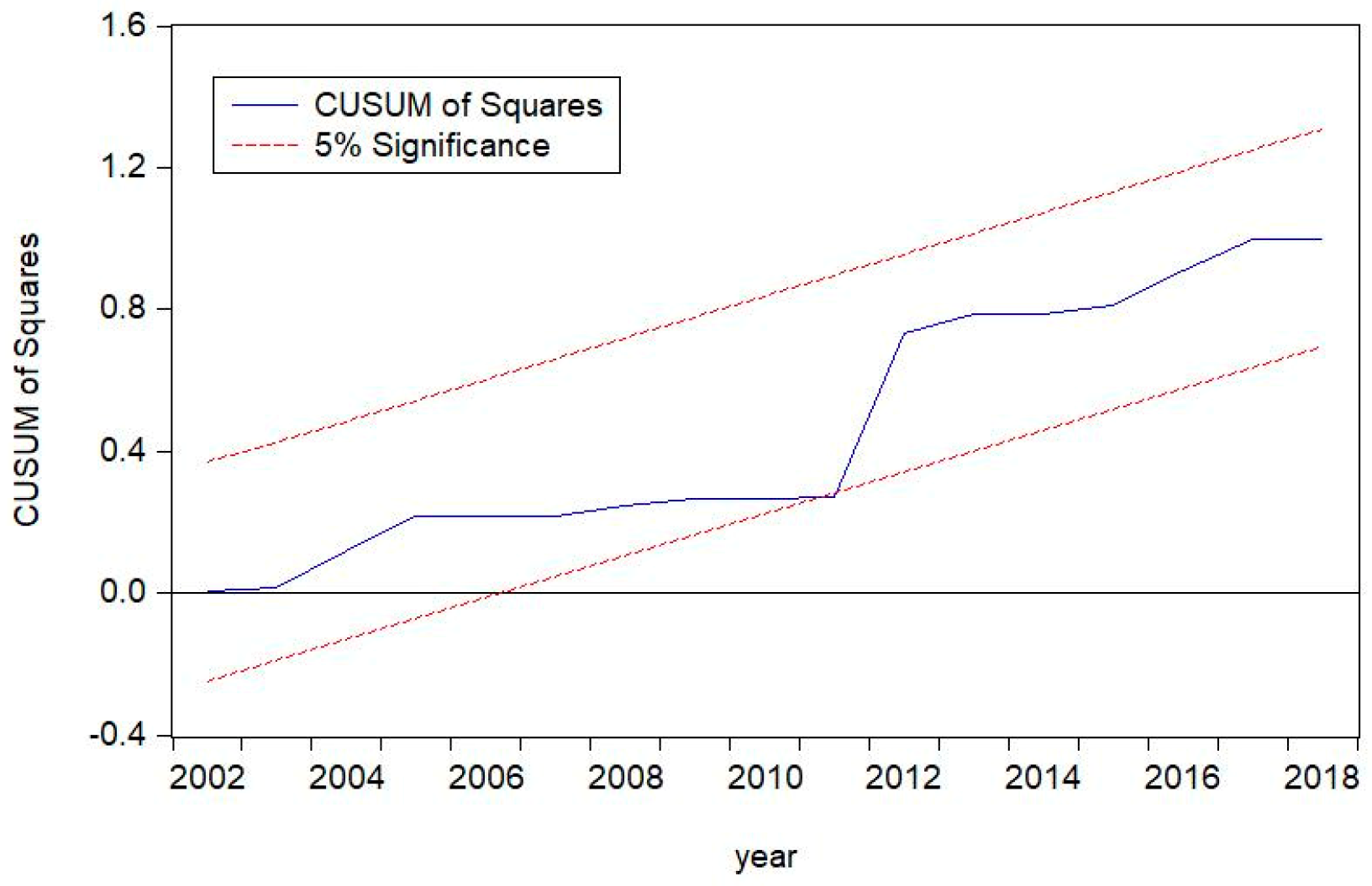
On the basis of this model, the stability of the selected model is tested by using the recursive residual accumulation sum test (CUSUM) and the recursive residual cumulative square sum test (CUSUM of squares). The results are shown in Figure 2 and Figure 3.

It can be seen from Figure 2 and Figure 3 that both statistics are within the $5\%$ significance lines, indicating that the parameters in the ARDL model are stable. From Table 4, the long-term co-integration equations for wind power development and carbon emissions can be obtained.

$$\ln X=6.1556\times \ln Y+68.9407$$

(8)

From the above formula, it can be seen that for every 1% increase in carbon emissions, $1\%$ of the growth rate of the newly installed of wind power capacity will increase by $6.1556\%$. It can be seen that the increase in carbon emissions will accelerate the development of wind power.

4.3. Granger Causality Analysis

Since there is a long-term co-integration relationship between China’s wind power development and carbon emissions, an error correction model can be used to analyse the Granger causal relationship between the two. We run the analysis using the Eviews software, and the results are shown in

Table 5. ECM-based Granger causality test results.

Pairwise Granger Causality Tests
Sample: 1990 2018
Lags: 4
Null Hypothesis	Obs	F-Statistic	Prob.
LNY does not Granger Cause LNX	24	3.42253	0.0354
LNX does not Granger Cause LNY		0.38472	0.8162

.

It can be seen from Table 5 that carbon emissions are the cause of wind power development, and wind power development will not increase carbon emissions, but it will inhibit carbon emissions and enable the environment to be effectively improved. Therefore, the growth of carbon emissions will drive the development of wind power, but the development of wind power will also inhibit the growth of carbon emissions, thereby reducing the speed of wind power development. In the long run, the final installed capacity of wind power will reach a certain value, and the amount of carbon emissions will be reduced to a certain value, achieving stable development.

5. Conclusions and Outlook

There have been a few scholars that have studied the relationship between a certain energy’s development and carbon emissions. Almost no research has been conducted on the relationship between wind power development and carbon emissions. Here, the relationship between wind power development and carbon emissions are effectively assessed using models and causality tests. The data we used are open to the public and published by the government, and the data source is authoritative and reliable.

Results are as follows.

1. The ARDL model verifies the long-term stable relationship between wind power development and carbon emissions reductions. The two interact with each other, and so the development of wind power will impact carbon emissions.

2. The Granger causality test shows that an increase in carbon emissions will contribute to the annual increase in the newly installed wind power capacity. The reductions in carbon emissions will also inhibit the development of wind power. In the long run, the two will eventually stabilize in a certain region and steadily develop. However, at present, global carbon emissions are always increasing, which will certainly drive the development of wind power. Therefore, countries around the world should increase investments related to wind power, promote wind power development, effectively curb the increase in carbon emissions, protect the environment, and conserve resources.

3. The excessive use of fossil energy makes greenhouse gas emissions harmful to the environment. The rapid growth of carbon emissions is one of the driving forces for our development of clean energy. To promote the sustainable development of China’s energy and alleviate the energy consumption crisis, China should promote the development of wind power and promote the utilization of renewable energy.

First, in order to promote sustainable energy development, alleviate environmental pollution and reduce carbon emissions, the Chinese government should vigorously develop wind power, increase investments in wind power development, and formulate relevant subsidy policies to promote the development of renewable energy. Second, the Chinese government is also facing the problem of wind power consumption, which was solved by the government through administrative means. Currently, China is in the stage of the power market reform, and the problem of wind power consumption should be solved through market means. This will be the focus of our future research.

References

- Gao, H.; Yang, W.; Yang, Y.; Yuan, G. Analysis of the Air Quality and the Effect of Governance Policies in China’s Pearl River Delta, 2015–2018. Atmosphere 2019, 10, 412. [Google Scholar] [CrossRef]
- Yang, W.X.; Li, L.G. Energy Efficiency, Ownership Structure, and Sustainable Development: Evidence from China. Sustainability 2017, 9, 912. [Google Scholar] [CrossRef]
- Yang, W.; Li, L. Analysis of Total Factor Efficiency of Water Resource and Energy in China: A Study Based on DEA-SBM Model. Sustainability 2017, 9, 1316. [Google Scholar] [CrossRef]
- Yuan, G.; Yang, W. Evaluating China’s Air Pollution Control Policy with Extended AQI Indicator System: Example of the Beijing-Tianjin-Hebei Region. Sustainability 2019, 11, 939. [Google Scholar] [CrossRef]
- Li, L.; Yang, W. Total Factor Efficiency Study on China’s Industrial Coal Input and Wastewater Control with Dual Target Variables. Sustainability 2018, 10, 2121. [Google Scholar] [CrossRef]
- Yang, W.; Li, L. Efficiency Evaluation and Policy Analysis of Industrial Wastewater Control in China. Energies 2017, 10, 1201. [Google Scholar] [CrossRef]
- Yang, W.; Li, L. Efficiency evaluation of industrial waste gas control in China: A study based on data envelopment analysis (DEA) model. J. Clean. Prod. 2018, 179, 1–11. [Google Scholar] [CrossRef]
- Yang, W.; Yuan, G.; Han, J. Is China’s air pollution control policy effective? Evidence from Yangtze River Delta cities. J. Clean. Prod. 2019, 220, 110–133. [Google Scholar] [CrossRef]
- Yuan, G.; Yang, W. Study on optimization of economic dispatching of electric power system based on Hybrid Intelligent Algorithms (PSO and AFSA). Energy 2019, 183, 926–935. [Google Scholar] [CrossRef]
- Yang, Y.; Yang, W. Does Whistleblowing Work for Air Pollution Control in China? A Study Based on Three-party Evolutionary Game Model under Incomplete Information. Sustainability 2019, 11, 324. [Google Scholar] [CrossRef]
- Gnatowska, R.; Moryń-Kucharczyk, E. Current status of wind energy policy in Poland. Renew. Energy 2019, 135, 232–237. [Google Scholar] [CrossRef]
- Jefferson, M. Renewable and low carbon technologies policy. Energy Policy 2018, 123, 367–372. [Google Scholar] [CrossRef]
- Wei, X.; Duan, Y.; Liu, Y.; Jin, S.; Sun, C. Onshore-offshore wind energy resource evaluation based on synergetic use of multiple satellite data and meteorological stations in Jiangsu Province, China. Front. Earth Sci. 2019, 13, 132–150. [Google Scholar] [CrossRef]
- Adefarati, T.; Bansal, R.C. Reliability, economic and environmental analysis of a microgrid system in the presence of renewable energy resources. Appl. Energy 2019, 236, 1089–1114. [Google Scholar] [CrossRef]
- Dalla Longa, F.; Strikkers, T.; Kober, T.; van der Zwaan, B. Advancing Energy Access Modelling with Geographic Information System Data. Environ. Model. Assess. 2018, 23, 627–637. [Google Scholar] [CrossRef] [Green Version]
- Ebrahimi, M.; Rahmani, D. A five-dimensional approach to sustainability for prioritizing energy production systems using a revised GRA method: A case study. Renew. Energy 2019, 135, 345–354. [Google Scholar] [CrossRef]
- Liu, Z.; Liu, Y.; He, B.-J.; Xu, W.; Jin, G.; Zhang, X. Application and suitability analysis of the key technologies in nearly zero energy buildings in China. Renew. Sustain. Energy Rev. 2019, 101, 329–345. [Google Scholar] [CrossRef]
- Bandoc, G.; Pravalie, R.; Patriche, C.; Degeratu, M. Spatial assessment of wind power potential at global scale. A geographical approach. J. Clean. Prod. 2018, 200, 1065–1086. [Google Scholar] [CrossRef]
- Liu, F.; Sun, F.; Liu, W.; Wang, T.; Wang, H.; Wang, X.; Lim, W.H. On wind speed pattern and energy potential in China. Appl. Energy 2019, 236, 867–876. [Google Scholar] [CrossRef]
- deCastro, M.; Costoya, X.; Salvador, S.; Carvalho, D.; Gomez-Gesteira, M.; Javier Sanz-Larruga, F.; Gimeno, L. An overview of offshore wind energy resources in Europe under present and future climate. Ann. N. Y. Acad. Sci. 2019, 1436, 70–97. [Google Scholar] [CrossRef]
- Li, X.; Feng, D.; Li, J.; Zhang, Z. Research on the Spatial Network Characteristics and Synergetic Abatement Effect of the Carbon Emissions in Beijing–Tianjin–Hebei Urban Agglomeration. Sustainability 2019, 11, 1444. [Google Scholar] [CrossRef]
- Liu, Y.; Hu, X.; Wu, H.; Zhang, A.; Feng, J.; Gong, J. Spatiotemporal Analysis of Carbon Emissions and Carbon Storage Using National Geography Census Data in Wuhan, China. ISPRS Int. J. Geo-Inf. 2019, 8, 7. [Google Scholar] [CrossRef]
- Martin, C.R.; Zeng, N.; Karion, A.; Mueller, K.; Ghosh, S.; Lopez-Coto, I.; Gurney, K.R.; Oda, T.; Prasad, K.; Liu, Y.; et al. Investigating sources of variability and error in simulations of carbon dioxide in an urban region. Atmos. Environ. 2019, 199, 55–69. [Google Scholar] [CrossRef]
- Xu, Q.; Dong, Y.; Yang, R.; Zhang, H.; Wang, C.; Du, Z. Temporal and spatial differences in carbon emissions in the Pearl River Delta based on multi-resolution emission inventory modeling. J. Clean. Prod. 2019, 214, 615–622. [Google Scholar] [CrossRef]
- Brouwer, A.S.; van den Broek, M.; Zappa, W.; Turkenburg, W.C.; Faaij, A. Least-cost options for integrating intermittent renewables in low-carbon power systems. Appl. Energy 2016, 161, 48–74. [Google Scholar] [CrossRef]
- Hanak, D.P.; Anthony, E.J.; Manovic, V. A review of developments in pilot-plant testing and modelling of calcium looping process for CO2 capture from power generation systems. Energy Environ. Sci. 2015, 8, 2199–2249. [Google Scholar] [CrossRef]
- Hertwich, E.G.; Gibon, T.; Bouman, E.A.; Arvesen, A.; Suh, S.; Heath, G.A.; Bergesen, J.D.; Ramirez, A.; Vega, M.I.; Shi, L. Integrated life-cycle assessment of electricity-supply scenarios confirms global environmental benefit of low-carbon technologies. Proc. Natl. Acad. Sci. USA 2015, 112, 6277–6282. [Google Scholar] [CrossRef] [PubMed]
- Foley, A.M.; Leahy, P.G.; Li, K.; McKeogh, E.J.; Morrison, A.P. A long-term analysis of pumped hydro storage to firm wind power. Appl. Energy 2015, 137, 638–648. [Google Scholar] [CrossRef]
- Guandalini, G.; Campanari, S.; Romano, M.C. Power-to-gas plants and gas turbines for improved wind energy dispatchability: Energy and economic assessment. Appl. Energy 2015, 147, 117–130. [Google Scholar] [CrossRef]
- Lund, P.D.; Mikkola, J.; Ypya, J. Smart energy system design for large clean power schemes in urban areas. J. Clean. Prod. 2015, 103, 437–445. [Google Scholar] [CrossRef]
- Sun, H.; Luo, X.; Wang, J. Feasibility study of a hybrid wind turbine system—Integration with compressed air energy storage. Appl. Energy 2015, 137, 617–628. [Google Scholar] [CrossRef]
- Boluk, G.; Mert, M. The renewable energy, growth and environmental Kuznets curve in Turkey: An ARDL approach. Renew. Sustain. Energy Rev. 2015, 52, 587–595. [Google Scholar] [CrossRef]
- Shahbaz, M.; Loganathan, N.; Muzaffar, A.T.; Ahmed, K.; Jabran, M.A. How urbanization affects CO2 emissions of STIRPAT model in Malaysia? The application. Renew. Sustain. Energy Rev. 2016, 57, 83–93. [Google Scholar] [CrossRef]
- Asumadu-Sarkodie, S.; Owusu, P.A. The relationship between carbon dioxide and agriculture in Ghana: A comparison of VECM and ARDL model. Environ. Sci. Pollut. Res. 2016, 23, 10968–10982. [Google Scholar] [CrossRef]
- Cerdeira Sento, J.P.; Moutinho, V. CO2 emissions, non-renewable and renewable electricity production, economic growth, and international trade in Italy. Renew. Sustain. Energy Rev. 2016, 55, 142–155. [Google Scholar] [CrossRef]
- Shahbaz, M.; Loganathan, N.; Zeshan, M.; Zaman, K. Does renewable energy consumption add in economic growth? An application of auto-regressive distributed lag model in Pakistan. Renew. Sustain. Energy Rev. 2015, 44, 576–585. [Google Scholar] [CrossRef]
- Asumadu-Sarkodie, S.; Owusu, P.A. Carbon dioxide emissions, GDP, energy use, and population growth: A multivariate and causality analysis for Ghana, 1971-2013. Environ. Sci. Pollut. Res. 2016, 23, 13508–13520. [Google Scholar] [CrossRef]
- Shahbaz, M.; Khraief, N.; Ben Jemaa, M.M. On the causal nexus of road transport CO2 emissions and macroeconomic variables in Tunisia: Evidence from combined cointegration tests. Renew. Sustain. Energy Rev. 2015, 51, 89–100. [Google Scholar] [CrossRef]
- Abbasi, F.; Riaz, I. CO2 emissions and financial development in an emerging economy: An augmented VAR approach. Energy Policy 2016, 90, 102–114. [Google Scholar] [CrossRef]
- Ahmad, N.; Du, L. Effects of energy production and CO2 emissions on economic growth in Iran: ARDL approach. Energy 2017, 123, 521–537. [Google Scholar] [CrossRef]
- Liu, X.; Bae, J. Urbanization and industrialization impact of CO2 emissions in China. J. Clean. Prod. 2018, 172, 178–186. [Google Scholar] [CrossRef]
- Sun, C.; Zhang, F.; Xu, M. Investigation of pollution haven hypothesis for China: An ARDL approach with breakpoint unit root tests. J. Clean. Prod. 2017, 161, 153–164. [Google Scholar] [CrossRef]
- Li, N.; Chen, M.Z.; Chen, M. Nonlinear Progress and Application Research of Granger Causality Test. J. Appl. Stat. Manag. 2017, 36, 891–905. [Google Scholar]
- Liu, H.; Wang, Y.L.; Chen, D.K. Analysis of the Efficacy and Robustness of Mixed Granger Causality Test. J. Quant. Tech. Econ. 2017, 34, 144–161. [Google Scholar]
- Dogan, E.; Turkekul, B. CO2 emissions, real output, energy consumption, trade, urbanization and financial development: Testing the EKC hypothesis for the USA. Environ. Sci. Pollut. Res. 2016, 23, 1203–1213. [Google Scholar] [CrossRef]
- Tang, C.F.; Tan, B.W. The impact of energy consumption, income and foreign direct investment on carbon dioxide emissions in Vietnam. Energy 2015, 79, 447–454. [Google Scholar] [CrossRef]
- Ben Jebli, M.; Ben Youssef, S.; Ozturk, I. Testing environmental Kuznets curve hypothesis: The role of renewable and non-renewable energy consumption and trade in OECD countries. Ecol. Indic. 2016, 60, 824–831. [Google Scholar] [CrossRef]
- Dogan, E. The relationship between economic growth and electricity consumption from renewable and non-renewable sources: A study of Turkey. Renew. Sustain. Energy Rev. 2015, 52, 534–546. [Google Scholar] [CrossRef]
- Seker, F.; Ertugrul, H.M.; Cetin, M. The impact of foreign direct investment on environmental quality: A bounds testing and causality analysis for Turkey. Renew. Sustain. Energy Rev. 2015, 52, 347–356. [Google Scholar] [CrossRef]
- Wang, Y.; Chen, L.; Kubota, J. The relationship between urbanization, energy use and carbon emissions: Evidence from a panel of Association of Southeast Asian Nations (ASEAN) countries. J. Clean. Prod. 2016, 112, 1368–1374. [Google Scholar] [CrossRef]
- Yousefi-Sahzabi, A.; Sasaki, K.; Yousefi, H.; Pirasteh, S.; Sugai, Y. GIS aided prediction of CO2 emission dispersion from geothermal electricity production. J. Clean. Prod. 2011, 19, 1982–1993. [Google Scholar] [CrossRef]
- Charenza, W.W.; Deadman, D.F. New Directions in Econometric Analysis; Oxford University Press: Oxford, UK, 1997. [Google Scholar]
- Pesaran, M.H.; Shin, Y.; Smith, R.J. Bounds testing approaches to the analysis of level relationships. J. Appl. Econom. 2001, 16, 289–326. [Google Scholar] [CrossRef]
- Ouattara, B. Foreign Aid and Fiscal Policy in Senegal; Mimeo University of Manchester: Manchester, UK, 2004. [Google Scholar]
Figure 1.
Annual carbon emissions and newly installed wind power capacity.
Figure 2.
CUSUM TEST.
Figure 3.
CUSUM of squares.