Using Pareto Optimization to Support Supply Chain Network Design within Environmental Footprint Impact Assessment


Department of Industrial and Systems Engineering, Chung Yuan Christian University, Taoyuan City 320, Taiwan
*
Author to whom correspondence should be addressed.
Sustainability 2019, 11(2), 452; https://doi.org/10.3390/su11020452
Submission received: 20 November 2018
/
Revised: 8 January 2019
/
Accepted: 15 January 2019
/
Published: 16 January 2019
(This article belongs to the Special Issue Carbon Footprint: As an Environmental Sustainability Indicator)
Abstract
:A product environmental footprint is a multi-criteria measure for environmental sustainability. Most of these environmental criteria are either synergies (non-trade-offs) or compromises (trade-offs) within environmental metrics. This forms a multi-objective problem of supply chain network design. The product environmental footprint is an aid or tool that enterprises may use to measure and improve the life cycle environmental performance of their products. In this research, a multi-criteria method, Pareto optimization, is used to design a supply chain network based on the results of a product environmental footprint. In Pareto optimization, two objectives are formulated: Environmental impact and cost. Using the results of this research, designers will be able to choose a material with a lower environmental impact and supply chain managers will be able to select suppliers with lower environmental impacts. A case study of industry practice is also analyzed. It shows an environmental footprint is useful for the supply chain design network.
1. Introduction
To reduce environmental impacts, several environmental footprints have been developed for enterprises to use in measuring aspects of environmental performance, such as the carbon footprint (CF) (ISO 14067: 2018) and water footprint (WF) (ISO 14046: 2014). In the past, these footprints provided significant contributions for assisting enterprises in obtaining measurements and achieving reductions in different markets [1,2]. However, given the existence of a variety of footprint indicators that measure single or collective pressures arising from production and consumption, an enterprise must choose only some of them to address the significant anthropogenic impacts on the ecosystem [3]. Therefore, it is necessary to develop an integrated footprint.
Product environmental footprints (PEFs) are used as criteria for environmental sustainability. Most of these criteria are either synergies (non-trade-offs) or compromises (trade-offs) within environmental metrics. For example, photovoltaics show synergies in the CF, WF, NF (nitrogen footprint), and ENF (energy footprint). In addition, when an enterprise attempts to improve the life cycle environmental performance of a product, most research highlights two objectives that must be addressed simultaneously: Lowered cost (the economic aspect) and reduced environmental impacts. This creates a multi-objective optimization (MOO) problem in a supply chain network design [4]. Supply chain network design, which determines the infrastructure and physical structure of a supply chain, is also called strategic supply planning [5], and covers the issues of efficiency and risk under uncertainty [6].
This research investigates a bi-objective optimization problem related to the design of a supply chain network to solve this trade-off problem. MOO is also used to determine the best solutions for the problem while considering the suppliers’ existing constraints [7], which include the suppliers’ environmental impacts, cost, and production capacities. The supply chain network design is determined through resolution of the MOO problem, which also allows selection of appropriate suppliers based on low environmental impact and cost.
The structure of this paper is as follows. First, a literature review on environmental footprints is presented. The next section describes the research methods used in this study. Finally, the empirical data are analyzed, and conclusions are drawn.
2. Literature Review
The goal of the literature review is to review relevant background material so as to identify gaps, weaknesses, problems or controversies that need to be addressed. The literature review is presented in two parts. The first part introduces the concept of a product environmental footprint, while the second part examines design for product environmental footprints.
2.1. Introduction of Product Environmental Footprints
The concept of an environmental “footprint” originated in 1992 based on the term “ecological footprint” [8]. Footprints can be presented as the planet’s boundaries, comprised of its biophysical subsystems or processes. Many footprints exist; however, not all have a standard and clear definition. Čuček et al. [9] summarized existing footprints based on a triple bottom line: economic, environmental, and social footprints. Product environmental impacts should consider the product’s whole life cycle through the methodology of life cycle analysis. The 14 impacts of the environmental footprint include: climate change, ozone depletion, human toxicity, cancer effects, non-cancer effects, particulate matter, ionizing radiation HH, photochemical ozone formation, acidification, terrestrial eutrophication, freshwater eutrophication, freshwater eco-toxicity, land use, water resource depletion, and mineral, fossil, and resource depletion. Table 1 shows the impact assessment model as updated in 2018 [10]. Based on the product environment guide [11], the PEF was initiated with the aim of developing a harmonized European methodology for environmental footprint (EF) studies that can accommodate a broader suite of relevant environmental performance criteria using a life-cycle approach. This methodology also considers ISO standards: ISO 14044 [12], ISO/DIS 14067 [13], ISO 14025 [14], ISO 14020 [15], greenhouse gas (GHG) protocol, the specification for assessment of the life cycle GHG emissions of goods and services [16], and the International Reference Life Cycle Data System (ILCD) handbook [17], among others.
2.2. Designing for Product Environmental Footprint
It is very important to systematically evaluate the product’s environmental footprint in the early design stage [18]. Previously, designers used qualitative and subjective methods that drew on their extensive experience and knowledge, such as checklists or design guidelines, to evaluate qualitative attributes for their environmental impacts [19,20,21]. However, as quantitative methods and tools have been further developed, designers have begun adopting these tools to support their design decisions, footprints, or determine the indicators of potential environmental impacts. These quantitative tools, the bottom-up life cycle assessment (LCA) and top-down input-output analysis (IOA), are important methodologies that support both designers and supply chain managers in decision making.
A significant number of studies are related to decreasing the environmental footprints of products. There are three approaches to decreasing an environmental footprint: low environmental impact (1) material substitution, (2) manufacturing process substitution, and (3) logistics design, such as low environmental impact supplier substitution. Together, these form a low carbon supply chain network design. A supply chain can be seen as a network of actors that perform the functions of product development, procurement of material from suppliers, movement of material between facilities, manufacturing and product distribution of finished goods to customers, and after-market support for sustainment [22,23]. Based on this definition, environmental impacts could be reduced through supplier integration [24].
Normally, it is difficult to evaluate a product’s environmental footprint during the concept design phase, since there may only be a rough idea of the solution without adequate and accurate operational data [25]. To solve this problem, Song and Lee [26] developed a low carbon product system that includes GHG-BOM (Bill of Material), estimation of the product’s GHG emissions, identification of problematics parts. Kuo et al. [1] developed a CO2 predictive system based on the depth-first search in the early design stage, while Hitchcock [27] developed low carbon and green supply chains. Yang et al. [28] used bilinear non-convex mixed integer programming, which was reduced to a pure linear mixed integer model for a low-carbon city logistics distribution network design. Kawasaki et al. [29] constructed a model to simulate the relationship of CO2 emissions, cost, and lead time. Tseng and Hung [30] developed an objective function that considered the operations and social costs of CO2 emissions, allowing evaluation of carbon emissions in greater detail through the life cycle stages. In Kuo et al.’s [31] model, a low carbon supply chain network was optimized based on carbon emissions, cost, and suppliers’ manufacturing capacities. However, when trade-offs exist between different life cycle stages or different product environmental footprints, a challenge remains.
In summary, two foundational research issues have been studied in relation to sustainable design synthesis to reduce environmental impacts [18]. One addresses the means by which a sustainable design can be created for a product’s environmental footprint and the generation of feasible solutions through design synthesis. The second, existing design methodology for determining low product environmental footprints, still lacks an optimal solution for the product life cycle.
3. Research Methods
3.1. Pareto-Optimal Solutions
Multi-objective optimization problems involve more than one objective function that is to be minimized or maximized. The answer is a set of solutions that define the best trade-off between competing objectives. There are some multi-objective methods such as the weighted sum method, weighted metric method. The challenge for the multi-objective is how to define the best trade-off between competing objectives. One way to resolve multi-objective problems is by using Pareto-optimal solutions. Normally, a multi-objective optimization problem can be formally defined as in Equation (1):
where x is the vector of decision variables bounded by the decision space, , and f is the set of objectives to be minimized [32]. The functions g(x) and h(x) respectively represent the sets of inequality and equality constraints that define the feasible region of the -dimensional continuous or discrete space. To solve a multi-objective optimization problem, Messac et al. [33] proposed the normal constraint method for generating a set of evenly spaced solutions on a Pareto frontier. The seven steps of the normal constraint method to generate a set of evenly spaced solutions on a Pareto frontier are as follows. Utopia line refers to the line joining two anchor points in bi-objective cases, where anchor point is defined as minimizer of the specific objective function with no regard to other objectives. Utopia hyperplane refers to the plane that comprises all the anchor points in the multi-objective case.
Step 1. Obtain anchor points,
Step 2. Objective mapping/normalization,
Step 3. Generate Utopia line vector,
Step 4. Normalize increments,
Step 5. Generate Utopia line points,
Step 6. Pareto point generation, and
Step 7. Pareto design metric values.
3.2. Variables
In this section, the symbol, parameter, and decision variable are introduced (Table 2).
3.3. Product Environmental Footprint Minimization and Cost Minimization
Suppose the supply chain manufacturer tries to minimize total environmental impacts and cost simultaneously, based on the quantity of material/components, transportation distance, power consumption of the manufacturing process, and production capacity of the supplier. Basically, the Product’s Environmental Footprint (PEF) is equal to as Equation (2):
where
PEF = AD × EF
AD: activity data, collected (measured, calculated, or estimated) from production sites associated with the unit processes within the system boundary
EF: emission factor, data derived from databases
3.3.1. Product Environmental Footprint
The EF is defined as follows. Equation (3) is the sum of the environmental impacts of raw material usage and processes.
where represents the environmental impacts for the raw material, and for the environmental impacts for the manufacturing process.
The supply chain manager will consider that the different materials in different production lines using different processes will have varied environmental impacts. Equation (4) is the sum of the environmental impacts of the manufacturing activities, machining processes, and so on.
The supply chain manager will also consider the environmental impacts of the main and sub materials. Equation (4) is the sum of the environmental impacts of raw material usage and processes, where is the environmental impact for the ith supplier with the kth material/components, is ton-kilometers for the ith supplier with the kth material/components, is the environmental impact for the jth transportation mode, and is the total environmental impact for sub materials, Equations (5)–(8).
, is weight for the kth material/component
3.3.2. Cost
Cost is defined as follows. Equation (9) is the sum of the environmental impacts of raw material usage and processes.
where = cost of total power consumption.
During the manufacturing process, the cost of different materials varies at different production lines using different processes. Equation (10) is the cost of total power consumption. Equations (10)–(11) are the costs of the main raw material, transportation, and sub materials.
3.3.3. Constraints
Equations (13)–(15) are the constraints for total cost and environmental impacts. Equation (13) shows that supply usage should be equal to that of demand. Equation (14) shows that total demand should be less than suppliers’ total production capacity, while Equation (15) shows that the supplier should provide a certain amount to be available for purchase.
4. Case Study
In this research, a case study is conducted of a type of gardening equipment, a gardening shear. The company is located in northern Taiwan. The scope of the life cycle inventory in this research is defined by the phrase, “from cradle to gate”. Figure 1 shows the production road map. Thus far, there is no product category rule for the gardening shear. The raw material includes 1 primary kind of material and 45 kinds of sub material. There are 51 suppliers that can supply the 46 materials.
4.1. Data Collection
To reduce environmental impacts, there are three alternatives that allow designers to select a suitable material: hot rolled steel, forged steel, and SK 85 fiber reinforced plastic. The production capacities for these three types of material are also limited to 75,000 pcs, 25,000 pcs, and 75,000 pcs, respectively. The total marketing demand is 100,000 pcs/month. To calculate the environmental footprint of the gardening equipment, the material data is extracted from the bill of material (BOM) in the enterprise resource planning system. The electricity usage is calculated based on the Tai-electricity bill in Taiwan. The ILCD 2011 midpoint method version 1.01 in SimaPro software is used to calculate the environmental impact [34]. The following data are collected from the case study. There are six different types of transportation: a truck weighing less than 3.5 tons (T1), a 3.5 ton truck (T2), an 11 ton truck (T3), a 15 ton truck (T4), sea transportation to Tokyo (T5), and sea transportation to Geneva (T6). Table 3 shows the suppliers for different materials as well as their transportation method. Most suppliers are located in Taiwan; however, S6 and S8 are outside of Taiwan.
Table 4 shows the supplier travel distance. Here, the ton-km is a unit of freight carriage that is equal to the transportation of one metric ton of freight over a distance of one kilometer. Table 5 shows the cost and weight of different materials, and Table 6 shows the cost of different transportation types.
5. Results
5.1. The EF Impacts
The environmental impacts are calculated based on ILCD 2011 midpoint method in Simapro software. From the lifecycle stages, most of the EF impacts are found in the raw material and manufacturing stages. Among the EF impacts in Table 7, the most significant impacts are human toxicity, non-cancer effects, and freshwater eco-toxicity. In Table 8, hot rolled steel has higher EF impacts when compared to the other two materials. However, from the perspective of climate change, forged steel has the lowest impact.
5.2. The Pareto Frontier
From the calculation, the first objective is to minimize total environmental impact, which is 121.4 PT. The second objective is to minimize total cost, which is 1,067,316 USD. The Pareto frontier is then divided by 20 points, which is shown in Table 9. The reason why it is divided by 20 points is to be equally distributed. The designer can determine his or her priority based on the sequence of hot rolled steel, fiber reinforced plastics, and forged steel, as shown in Figure 2.
5.3. Discussion
Sustainable development goals have become a popular topic in the domain of sustainable development. Environmental footprint is a multi-objective problem. This study aimed to bridge the gap between theoretical and practical problems of environmental footprints. From Table 6, it could be concluded that most environmental impacts are from the “manufacturing stage”, and most of the environmental impacts of the “manufacturing stage” are from the energy used. If the enterprise wants to reduce the environmental impacts, the core strategy is to reduce the energy usage. In addition, the normal constraint method should yield multiple Pareto-optimal solutions rather than a single solution. Many studies only consider evaluation of carbon emissions. However, in this study, the supplier’s manufacturing capacity and location are also considered. To sum up, the method of Pareto optimization provides a group of solutions for the reference of the enterprise. The enterprise could select its suitable solution based on the enterprise strategy. In Figure 2, the solution is not easily identifiable for the enterprise since there is no obviously solution for the 20 points. It means the enterprise could decide how much they wanted to improve their environmental footprint. Compared with 20 points, points 1–6 represent a much more significant environmental footprint improvement.
6. Conclusions
Based on this research, supply chain managers can use the Pareto frontier to select materials and suppliers based on their environmental policies. Moreover, this calculation can be performed very quickly based on the supplier’s capacity, showing that the PEF is a useful tool to help enterprises economically reduce their environmental impacts. This research could be a very useful tool for the manager to estimate his/her supply chain network design.
For sustainable development goal 12 (ensure sustainable consumption and production patterns), enterprises need to address the challenges linked to air, soil, and water pollution, as well as exposure to toxic chemicals, under the auspices of multilateral environmental agreements. In the past, many studies have examined carbon reduction in supply chain network design, but few have considered environmental footprint optimization. As an environmental footprint study, this research is one of the industry pioneers for supply chain network design. Compared to research on carbon emissions reduction [27,31,35,36,37,38], this study more widely considers environmental impact reduction.
In general, there are three different ways to reduce environmental impacts. The first is to change to a material with a lower environmental impact. The second is to reduce the environmental impact of the process, while the third is to design supply chain networks with lower environmental impact. As Kuo et al. [32] mentioned, proper optimization of the supply chain may decrease its emissions. In this research, we used the Pareto frontier approach to investigate bi-objective supply chain network design and obtain uniform non-dominated Pareto solutions, which is the main contribution of this research to previous literature related to the use of multi-objective models for low environmental impact supply chain network design. These results are consistent with other studies.
Although the proposed optimization model is a noteworthy contribution to the literature on low environmental impact network design, it has its limitations. First, the case used is very simple, as some issues of uncertainty and risk level are not considered. Second, it only considers the aspect of electricity. For future research, we suggest that researchers consider different levels of design criteria and examine a more sophisticated case.
Author Contributions
T.C.K. designed the research; T.C.K. and Y.L. performed the research; Y.L. collected and analyzed data from industry practice; T.C.K. and Y.L. wrote the paper; finally, T.C.K. revised the paper. All authors have read and approved the final manuscript.
Funding
The authors would like to thank the Ministry of Science Technology of the Republic of China, Taiwan for financially supporting this research under contract MOST 107-2621-M-033-001.
Conflicts of Interest
The authors declare no conflict of interest.
References
- Kuo, T.C.; Smith, S.; Smith, G.C.; Huang, S.H. A predictive product attribute driven eco-design process using depth-first search. J. Clean. Prod. 2016, 112 Pt 4, 3201–3210. [Google Scholar] [CrossRef]
- Kuo, T.; Chen, H.; Liu, C.; Tu, J.-C.; Yeh, T.-C. Applying multi-objective planning in low-carbon product design. Int. J. Precis. Eng. Manuf. 2014, 15, 241–249. [Google Scholar] [CrossRef]
- Fang, K.; Heijungs, R.; de Snoo, G.R. Theoretical exploration for the combination of the ecological, energy, carbon, and water footprints: Overview of a footprint family. Ecol. Indic. 2014, 36, 508–518. [Google Scholar] [CrossRef]
- LCEP. On the Use of Common Methods to Measure and Communicate the Life Cycle Environmental Performance of Products and Organisations; European Commission: Brussels, Belgium, 2013. [Google Scholar]
- Cerchione, R.; Esposito, E. A systematic review of supply chain knowledge management research: State of the art and research opportunities. Int. J. Prod. Econ. 2016, 182, 276–292. [Google Scholar] [CrossRef]
- Govindan, K.; Fattahi, M.; Keyvanshokooh, E. Supply chain network design under uncertainty: A comprehensive review and future research directions. Eur. J. Oper. Res. 2017, 263, 108–141. [Google Scholar] [CrossRef]
- Rezapour, S.; Farahani, R.Z.; Pourakbar, M. Resilient supply chain network design under competition: A case study. Eur. J. Oper. Res. 2017, 259, 1017–1035. [Google Scholar] [CrossRef]
- Klemes, J. Introduction and Definition of the Field. In Sustainability in the Process Industry: Integration and Optimization; McGraw Hill Professional: New York, NY, USA, 2011. [Google Scholar]
- Rees, W.E. Ecological footprints and appropriated carrying capacity: What urban economics leaves out. Sustain. Cities 1992, 4, 121–130. [Google Scholar] [CrossRef]
- Čuček, L.; Klemeš, J.J.; Kravanja, Z. A Review of Footprint analysis tools for monitoring impacts on sustainability. J. Clean. Prod. 2012, 34, 9–20. [Google Scholar] [CrossRef]
- EC. Product Environmental Footprint (PEF) Guide. 2012. Available online: http://ec.europa.eu/environment/eussd/pdf/footprint/PEF%20methodology%20final%20draft.pdf (accessed on 14 January 2019).
- ISO. ISO 14044:2006 Environmental Management—Life Cycle Assessment—Requirements and Guidelines; ISO: Geneva, Switzerland, 2006. [Google Scholar]
- ISO. ISO/TR 14047:2012 Environmental Management—Life Cycle Assessment—Illustrative Examples on How to Apply ISO 14044 to Impact Assessment Situations; ISO: Geneva, Switzerland, 2012. [Google Scholar]
- ISO. ISO 14025:2006 Environmental Labels and Declarations—Type III Environmental Declarations—Principles and Procedures; ISO: Geneva, Switzerland, 2006. [Google Scholar]
- ISO. ISO 14020:2000 Environmental Labels and Declarations—General Principles; ISO: Geneva, Switzerland, 2000. [Google Scholar]
- BSI. PAS 2050 Specification for the Assessment of the Life Cycle Greenhouse Gas Emissions of Goods and Services; BSI British Standards: London, UK, 2008. [Google Scholar]
- EC. The International Reference Life Cycle Data System (ILCD) Handbook; Institute for Environment and Sustainability in the European Commission Joint Research Centre (JRC): Brussels, Belgium, 2012. [Google Scholar]
- He, B.; Gu, Z. Sustainable design synthesis for product environmental footprints. Des. Stud. 2016, 45, 159–186. [Google Scholar] [CrossRef]
- Kuo, T.-C.; Chang, S.-H.; Huang, S.H. Environmentally conscious design by using fuzzy multi-attribute decision-making. Int. J. Adv. Manuf. Technol. 2006, 29, 419–425. [Google Scholar] [CrossRef]
- Kuo, T.-C.; Wu, H.-H.; Shieh, J.-I. Integration of environmental considerations in quality function deployment by using fuzzy logic. Expert Syst. Appl. 2009, 36, 7148–7156. [Google Scholar] [CrossRef]
- Kuo, T.C. Enhancing disassembly and recycling planning using life-cycle analysis. Robot. Comput.-Integr. Manuf. 2006, 22, 420–428. [Google Scholar] [CrossRef]
- Hult, G.T.M.; Ketchen, D.J.; Slater, S.F. Information processing, knowledge development, and strategic supply chain performance. Acad. Manag. J. 2004, 47, 241–253. [Google Scholar]
- Hult, G.T.M.; Ketchen, D.J.; Cavusgil, S.T.; Calantone, R.J. Knowledge as a strategic resource in supply chains. J. Oper. Manag. 2006, 24, 458–475. [Google Scholar] [CrossRef]
- Handfield, R.B.; Cousins, P.D.; Lawson, B.; Petersen, K.J. How Can Supply Management Really Improve Performance? A Knowledge-Based Model of Alignment Capabilities. J. Supply Chain Manag. 2015, 51, 3–17. [Google Scholar] [CrossRef]
- He, B.; Xiao, J.; Deng, Z. Product design evaluation for product environmental footprint. J. Clean. Prod. 2018, 172, 3066–3080. [Google Scholar] [CrossRef]
- Song, J.-S.; Lee, K.-M. Development of a low-carbon product design system based on embedded GHG emissions. Resour. Conserv. Recycl. 2010, 54, 547–556. [Google Scholar] [CrossRef]
- Hitchcock, T. Low carbon and green supply chains: The legal drivers and commercial pressures. Supply Chain Manag. Int. J. 2012, 17, 98–101. [Google Scholar] [CrossRef]
- Yang, J.; Guo, J.; Ma, S. Low-carbon city logistics distribution network design with resource deployment. J. Clean. Prod. 2016, 119, 223–228. [Google Scholar] [CrossRef]
- Kawasaki, T.; Yamada, T.; Itsubo, N.; Inoue, M. Multi criteria simulation model for lead times, costs and CO2 emissions in a low-carbon supply chain network. Procedia CIRP 2015, 26, 329–334. [Google Scholar] [CrossRef]
- Tseng, S.-C.; Hung, S.-W. A strategic decision-making model considering the social costs of carbon dioxide emissions for sustainable supply chain management. J. Environ. Manag. 2014, 133, 315–322. [Google Scholar] [CrossRef] [PubMed]
- Kuo, T.C. The construction of a collaborative framework in support of low carbon product design. Robot. Comput. Integr. Manuf. 2013, 29, 174–183. [Google Scholar] [CrossRef]
- Kuo, T.-C.; Tseng, M.-L.; Chen, H.-M.; Chen, P.-S.; Chang, P.-C. Design and Analysis of Supply Chain Networks with Low Carbon Emissions. Comput. Econ. 2018, 52, 1353–1374. [Google Scholar] [CrossRef]
- Messac, A.; Ismail-Yahaya, A.; Mattson, C.A. The normalized normal constraint method for generating the Pareto frontier. Struct. Multidisc. Optim. 2003, 25, 86–98. [Google Scholar] [CrossRef]
- ILCD. Update of the ILCD 2011 Midpoint Method Version 1.04 in SimaPro. Available online: https://www.pre-sustainability.com/news/update-of-the-ilcd-2011-midpoint-method-version-104-in-simapro (accessed on 14 January 2019).
- Sundarakani, B.; de Souza, R.; Goh, M.; Wagner, S.M.; Manikandan, S. Modeling carbon footprints across the supply chain. Int. J. Prod. Econ. 2010, 128, 43–50. [Google Scholar] [CrossRef]
- Hua, G.; Cheng, T.C.E.; Wang, S. Managing carbon footprints in inventory management. Int. J. Prod. Econ. 2011, 132, 178–185. [Google Scholar] [CrossRef]
- Lee, K.H.; Cheong, I.M. Measuring a carbon footprint and environmental practice: The case of Hyundai Motors Co. (HMC). Ind. Manag. Data Syst. 2011, 111, 961–978. [Google Scholar] [CrossRef]
- Kannan, D.; Diabat, A.; Alrefaei, M.; Govindan, K.; Yong, G. A carbon footprint based reverse logistics network design model. Resour. Conserv. Recycl. 2012, 67, 75–79. [Google Scholar] [CrossRef]
Figure 1.
Production road map.
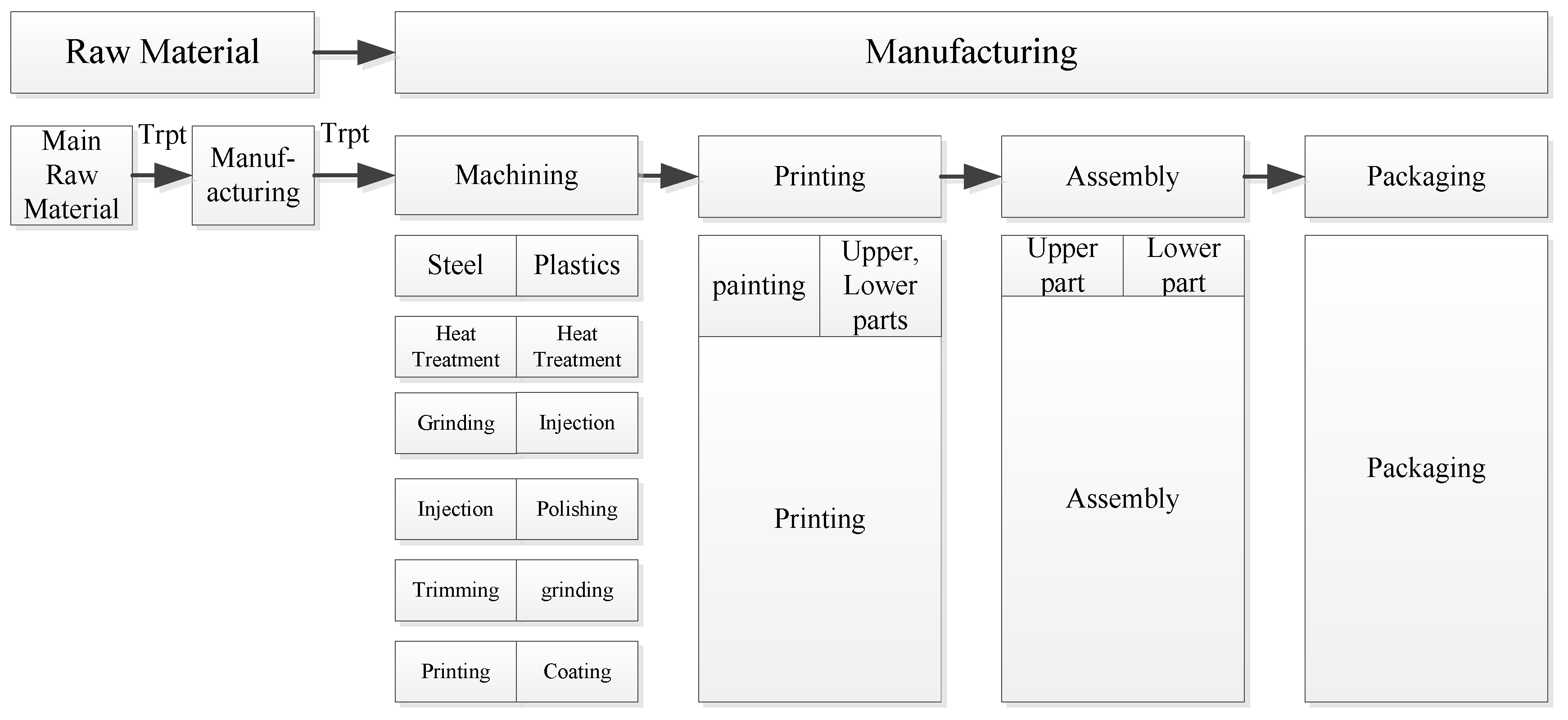
Figure 2.
EF & Cost of Pareto frontier.


Table 1.
Product environmental footprint (PEF) Methodology.
| NO | Impact Category | Impact Assessment Model | Impact Category Indicators |
|---|---|---|---|
| 1 | Climate Change | Global Warming Potentials (GWP) over a 100 year time horizon. IPCC 2013 | kg CO2 equivalent |
| 2 | Ozone Depletion | EDIP model based on the ODPs of the World Meteorological Organization (WMO) over an infinite time horizon. | kg CFC-11 equivalent |
| 3 | Ecotoxicity for aquatic fresh water | USEtox model | CTUe (Comparative Toxic Unit for ecosystems) |
| 4 | Human Toxicity—cancer effects | USEtox model | CTUh (Comparative Toxic Unit for humans) |
| 5 | Human Toxicity—non-cancer effects | USEtox model | CTUh (Comparative Toxic Unit for humans) |
| 6 | Particulate Matter/Respiratory Inorganics | Fantke et al. (2016) in UNEP (2016) | kg PM2.5 equivalent |
| 7 | Ionising Radiation—human health effects | Human Health effect model | Kg U235 equivalent |
| 8 | Photochemical Ozone Formation | LOTOS-EUROS model | kg NMVOC equivalent |
| 9 | Acidification | Accumulated Exceedance model | mol H+ eq |
| 10 | Eutrophication—terrestrial | Accumulated Exceedance model | mol N eq |
| 11 | Eutrophication—aquatic (fresh water) | EUTREND model | kg P equivalent |
| 12 | Resource Depletion—water | Available WAter Remaining (AWARE) model (UNEP 2016). | kg world deprived |
| 13 | Resource Depletion—fossil | CML method v. 4.8 (2016) | MJ |
| 14 | Land Transformation | LANCA LCIA model (as in Bos et al., 2016) | Kg |
Table 2.
Summary of symbols
| Symbol | Description |
| i | ith supplier, S = |
| j | jth transportation mode, T = |
| K | kth material/components, R = |
| a | ath production line, L = |
| b | bth process, M = |
| Parameter | |
| Environmental impacts of ith supplier, jth transportation mode, and kth material/component | |
| Total material demand | |
| Amount for ith supplier with kth material/component | |
| Ton-kilometer for ith supplier with kth material/component | |
| Total environmental impact for the sub material | |
| Environmental impact for ith supplier with kth material/component | |
| Weight of the kth material/component | |
| Di | Distance of the ith supplier |
| Environmental impact for the jth mode of transportation | |
| Environmental impact of Taiwan power | |
| Total Environmental impact of the process | |
| Power required for ath production line in bth process | |
| Environmental impact of ith supplier with kth sub material | |
| Ton-kilometer for ith supplier with kth sub material | |
| Weight of kth sub material | |
| Distance of the ith sub material supplier | |
| Environmental impact of the jth transportation mode of sub material | |
| Cost of ith supplier, jth transportation mode, and kth material/component | |
| Total manufacturing cost | |
| Total sub material cost | |
| Cost for the ith supplier with kth material/component | |
| Cost of the jth transportation mode | |
| Cost of the Taiwan power | |
| Cost for the ith supplier with kth sub material/component | |
| Cost of jth transportation mode of sub material | |
| Capacity of the ith supplier with kth material/component | |
| Decision variable | |
| Amount of ith supplier, jth transportation mode, and kth material/component | |
Table 3.
Data of the material/component supplier.
| Supplier | Material | Transportation | Material/Component | Supplier | Material | Transportation | Material/Component |
|---|---|---|---|---|---|---|---|
| S1 | R1 | T3 | hot rolled steel | S27 | R24 | T2 | Lubricating oil |
| S2 | R2 | T4 | forged steel | S28 | R25 | T2 | Lubricating oil |
| S3 | R3 | T2 | fiber reinforced plastic | S29 | R26 | T2 | Lubricating oil |
| S4 | R4 | T2 | Plastics (A) | S30 | R27 | T2 | Lubricating oil |
| S5 | R5 | T2 | Plastics (B) | S31 | R28 | T1 | Printing |
| S6 | R6 | T6 | Printing (A) | S32 | R29 | T1 | Printing |
| S7 | R6 | T2 | Printing (A) | S33 | R30 | T1 | Printing |
| S8 | R7 | T6 | Printing (B) | S34 | R31 | T1 | Printing |
| S9 | R7 | T2 | Printing (B) | S35 | R32 | T1 | Oil |
| S10 | R8 | T2 | Coating X | S36 | R33 | T2 | Packaging A |
| S11 | R9 | T2 | Coating Y | S37 | R34 | T2 | Packaging B |
| S12 | R10 | T2 | Steel sand (A) | S38 | R35 | T1 | Packaging C |
| S13 | R11 | T2 | Steel sand (B) | S39 | R36 | T2 | Packaging D |
| S14 | R12 | T1 | Screw | S40 | R37 | T2 | Packaging E |
| S15 | R13 | T1 | Nut | S41 | R38 | T2 | M3 screw |
| S16 | R14 | T1 | Spring | S42 | R39 | T1 | Packaging G |
| S17 | R15 | T2 | Switch | S43 | R40 | T1 | Packaging H |
| S18 | R16 | T1 | Lubricating oil | S44 | R41 | T2 | Packaging I |
| S19 | R17 | T5 | Oil for treatment | S45 | R42 | T2 | Packaging J |
| S20 | R18 | T2 | Grinding tool (A) | S46 | R43 | T2 | Packaging K |
| S21 | R18 | T2 | Grinding tool (B) | S47 | R44 | T1 | Tape 1.5 cm |
| S22 | R19 | T2 | Lubricating oil | S48 | R44 | T1 | Tape 1.5 cm |
| S23 | R20 | T2 | Lubricating oil | S49 | R45 | T1 | Tape 2 cm |
| S24 | R21 | T2 | Lubricating oil | S50 | R45 | T1 | Tape 2 cm |
| S25 | R22 | T2 | Lubricating oil | S51 | R46 | T1 | PE film |
| S26 | R23 | T2 | Lubricating oil |
Table 4.
Data of supplier travel distance.
| Supplier | Distance | Ton-km | Supplier | Distance | Ton-km | Supplier | Distance | Ton-km |
|---|---|---|---|---|---|---|---|---|
| S1 | 21.1 | 4.90 × 10⁻³ | S18 | 1.4 | 2.23 × 10⁻⁸ | S35 | 1.5 | 8.31 × 10⁻¹⁰ |
| S2 | 36.6 | 8.50 × 10⁻³ | S19 | 1450.91 | 1.66 × 10⁻⁴ | S36 | 2.3 | 1.07 × 10⁻⁵ |
| S3 | 24.7 | 5.74 × 10⁻³ | S20 | 25.1 | 2.87 × 10⁻⁶ | S37 | 20 | 1.51 × 10⁻⁴ |
| S4 | 1.3 | 4.72 × 10⁻⁵ | S21 | 144 | 1.70 × 10⁻⁴ | S38 | 6.2 | 4.96 × 10⁻⁶ |
| S5 | 30.2 | 1.10 × 10⁻³ | S22 | 17.2 | 2.35 × 10⁻⁵ | S39 | 19.8 | 1.65 × 10⁻⁴ |
| S6 | 9447.23 | 1.35 × 10⁻² | S23 | 26.5 | 1.45 × 10⁻⁶ | S40 | 10.2 | 1.01 × 10⁻⁴ |
| S7 | 19.4 | 2.77 × 10⁻⁵ | S24 | 17.2 | 1.26 × 10⁻⁶ | S41 | 10.2 | 1.45 × 10⁻⁴ |
| S8 | 9447.23 | 1.35 × 10⁻² | S25 | 26.5 | 2.15 × 10⁻⁶ | S42 | 8.4 | 1.81 × 10⁻⁶ |
| S9 | 34.3 | 4.89 × 10⁻⁵ | S26 | 17.2 | 1.79 × 10⁻⁶ | S43 | 8.4 | 1.08 × 10⁻⁶ |
| S10 | 7.3 | 1.58 × 10⁻⁶ | S27 | 16.1 | 5.08 × 10⁻⁶ | S44 | 10.2 | 4.89 × 10⁻⁶ |
| S11 | 7.3 | 1.24 × 10⁻⁵ | S28 | 17.2 | 5.42 × 10⁻⁶ | S45 | 10.2 | 3.93 × 10⁻⁶ |
| S12 | 24.8 | 1.32 × 10⁻³ | S29 | 6.8 | 2.77 × 10⁻⁷ | S46 | 21.2 | 3.17 × 10⁻⁶ |
| S13 | 36.3 | 1.96 × 10⁻³ | S30 | 5.9 | 2.30 × 10⁻⁷ | S47 | 13.8 | 5.21 × 10⁻⁶ |
| S14 | 5.6 | 4.59 × 10⁻⁵ | S31 | 156 | 4.68 × 10⁻⁷ | S48 | 27.2 | 1.03 × 10⁻⁵ |
| S15 | 5.6 | 1.26 × 10⁻⁵ | S32 | 156 | 2.11 × 10⁻⁷ | S49 | 13.8 | 3.38 × 10⁻⁶ |
| S16 | 14 | 1.68 × 10⁻⁵ | S33 | 16.7 | 1.50 × 10⁻⁷ | S50 | 27.2 | 6.65 × 10⁻⁶ |
| S17 | 12.1 | 4.34 × 10⁻⁵ | S34 | 16.7 | 3.76 × 10⁻⁷ | S51 | 27.2 | 9.19 × 10⁻⁷ |
Table 5.
Cost and weight of different materials.
| Material | Cost USD | Weight ton | Environmental Impact (PT) | Material | Cost USD | Weight ton | Environmental Impact (PT) |
|---|---|---|---|---|---|---|---|
| R1 | 0.139 | 2.32 × 10⁻⁴ | 2.23 × 10⁻⁴ | R24 | 0.0182 | 3.16 × 10⁻⁷ | 2.73 × 10⁻⁷ |
| R2 | 1.500 | 2.32 × 10⁻⁴ | 3.77 × 10⁻⁴ | R25 | 0.0182 | 3.15 × 10⁻⁷ | 2.72 × 10⁻⁷ |
| R3 | 5.066 | 2.32 × 10⁻⁴ | 3.36 × 10⁻⁵ | R26 | 0.0001 | 4.07 × 10⁻⁸ | 9.37 × 10⁻⁹ |
| R4 | 0.0602 | 3.63 × 10⁻⁵ | 7.68 × 10⁻⁶ | R27 | 0.0001 | 3.91 × 10⁻⁸ | 8.98 × 10⁻⁹ |
| R5 | 0.0603 | 3.64 × 10⁻⁵ | 7.70 × 10⁻⁶ | R28 | 0.0002 | 3 × 10⁻⁹ | 2.52 × 10⁻⁹ |
| R6 | 0.0327 | 1.43 × 10⁻⁶ | 7.52 × 10⁻⁷ | R29 | 0.0000 | 1.35 × 10⁻⁹ | 5.52 × 10⁻¹⁰ |
| R7 | 0.0326 | 1.43 × 10⁻⁶ | 8.44 × 10⁻⁷ | R30 | 0.0001 | 9.01 × 10⁻⁹ | 1.54 × 10⁻⁹ |
| R8 | 0.0078 | 2.16 × 10⁻⁷ | 1.97 × 10⁻⁸ | R31 | 0.0001 | 2.25 × 10⁻⁸ | 4.11 × 10⁻⁹ |
| R9 | 0.0615 | 1.7 × 10⁻⁶ | 1.76 × 10⁻⁵ | R32 | 0.0000 | 5.54 × 10⁻¹⁰ | 6.33 × 10⁻¹¹ |
| R10 | 2.7380 | 5.33 × 10⁻⁵ | 2.06 × 10⁻⁵ | R33 | 0.0026 | 4.67 × 10⁻⁶ | 2.89 × 10⁻⁶ |
| R11 | 2.7787 | 5.41 × 10⁻⁵ | 2.09 × 10⁻⁵ | R34 | 0.0432 | 7.53 × 10⁻⁶ | 3.20 × 10⁻⁶ |
| R12 | 0.0049 | 8.19 × 10⁻⁶ | 3.17 × 10⁻⁶ | R35 | 0.0005 | 8 × 10⁻⁷ | 3.10 × 10⁻⁷ |
| R13 | 0.0014 | 2.25 × 10⁻⁶ | 8.73 × 10⁻⁷ | R36 | 0.0019 | 8.32 × 10⁻⁶ | 1.24 × 10⁻⁹ |
| R14 | 0.0007 | 1.2 × 10⁻⁶ | 4.65 × 10⁻⁷ | R37 | 0.0857 | 9.86 × 10⁻⁶ | 4.19 × 10⁻⁶ |
| R15 | 0.0782 | 3.58 × 10⁻⁶ | 5.18 × 10⁻⁷ | R38 | 0.0399 | 1.43 × 10⁻⁵ | 6.06 × 10⁻⁶ |
| R16 | 0.0001 | 1.6 × 10⁻⁸ | 3.67 × 10⁻⁹ | R39 | 0.0121 | 2.15 × 10⁻⁷ | 3.68 × 10⁻⁸ |
| R17 | 0.0000 | 1.14 × 10⁻⁷ | 3.07 × 10⁻⁸ | R40 | 0.0072 | 1.28 × 10⁻⁷ | 2.20 × 10⁻⁸ |
| R18 | 0.0203 | 1.18 × 10⁻⁶ | 2.52 × 10⁻⁶ | R41 | 0.0045 | 4.79 × 10⁻⁷ | 1.28 × 10⁻⁷ |
| R19 | 0.0234 | 1.37 × 10⁻⁶ | 2.91 × 10⁻⁶ | R42 | 0.0005 | 3.85 × 10⁻⁷ | 1.64 × 10⁻⁷ |
| R20 | 0.0002 | 5.46 × 10⁻⁸ | 6.96 × 10⁻⁹ | R43 | 0.0009 | 1.49 × 10⁻⁷ | 4.48 × 10⁻⁸ |
| R21 | 0.0003 | 7.32 × 10⁻⁸ | 9.33 × 10⁻⁹ | R44 | 0.0046 | 3.78 × 10⁻⁷ | 8.44 × 10⁻⁹ |
| R22 | 0.0003 | 8.13 × 10⁻⁸ | 1.08 × 10⁻⁸ | R45 | 0.0023 | 2.45 × 10⁻⁷ | 5.47 × 10⁻⁹ |
| R23 | 0.0004 | 1.04 × 10⁻⁷ | 1.27 × 10⁻⁸ | R46 | 0.0001 | 3.38 × 10⁻⁸ | 1.26 × 10⁻⁸ |
Table 6.
Cost of different transportation types.
| Transportation Type | Environmental Impact Coefficient (PT) | Cost (USD) | Transportation Type | Environmental Impact Coefficient (PT) | Cost (USD) |
|---|---|---|---|---|---|
| T1 | 2.17 × 10⁻⁵ | 0.0002 | T4 | 3.16 × 10⁻⁵ | 0.0005 |
| T2 | 9.26 × 10⁻⁵ | 0.0002 | T5 | 6.60 × 10⁻⁷ | 0.0009 |
| T3 | 3.16 × 10⁻⁵ | 0.0004 | T6 | 6.60 × 10⁻⁷ | 0.0007 |
Table 7.
Environmental footprint (EF) of different life cycle stages.
| EF impacts | Raw Material | Transportation | Manufacturing | PT sub sum |
|---|---|---|---|---|
| Climate change | 1.18 × 10⁻⁵ | 6.43 × 10⁻⁸ | 3.07 × 10⁻⁵ | 4.25 × 10⁻⁵ |
| Ozone depletion | 2.63 × 10⁻⁷ | 4.77 × 10⁻⁹ | 5.10 × 10⁻⁷ | 7.78 × 10⁻⁷ |
| Human toxicity, cancer effects | 4.99 × 10⁻⁵ | 2.5 × 10⁻⁷ | 9.53 × 10⁻⁵ | 1.46 × 10⁻⁴ |
| Human toxicity, non-cancer effects | 4.58 × 10⁻⁴ | 6.56 × 10⁻⁷ | 3.91 × 10⁻⁴ | 8.49 × 10⁻⁴ |
| Particulate matter | 1.75 × 10⁻⁵ | 6.74 × 10⁻⁸ | 4.55 × 10⁻⁵ | 6.31 × 10⁻⁵ |
| Ionizing radiation | 9.67 × 10⁻⁶ | 3.87 × 10⁻⁸ | 5.32 × 10⁻⁵ | 6.3 × 10⁻⁵ |
| Photochemical ozone formation | 9.2 × 10⁻⁶ | 4.11 × 10⁻⁸ | 1.54 × 10⁻⁵ | 2.47 × 10⁻⁵ |
| Acidification | 1.18 × 10⁻⁵ | 4.32 × 10⁻⁸ | 2.58 × 10⁻⁵ | 3.76 × 10⁻⁵ |
| Terrestrial eutrophication | 4.45 × 10⁻⁶ | 2.02 × 10⁻⁸ | 9.52 × 10⁻⁶ | 1.4 × 10⁻⁵ |
| Freshwater eutrophication | 1.95 × 10⁻⁵ | 4.06 × 10⁻⁸ | 1.31 × 10⁻⁴ | 1.5 × 10⁻⁴ |
| Freshwater ecotoxicity | 1.93 × 10⁻⁴ | 4.58 × 10⁻⁷ | 1.54 × 10⁻⁴ | 3.47 × 10⁻⁴ |
| Land use | 1.32 × 10⁻⁶ | 2.55 × 10⁻⁸ | 2.02 × 10⁻⁶ | 3.37 × 10⁻⁶ |
| Water resource depletion | 1.7 × 10⁻⁵ | 8.39 × 10⁻¹⁰ | 1.50 × 10⁻⁶ | 1.85 × 10⁻⁵ |
| Mineral, fossil & ren resource depletion | 3.88 × 10⁻⁵ | 6.07 × 10⁻⁷ | 7.16 × 10⁻⁶ | 4.65 × 10⁻⁵ |
| Total | 8.42 × 10⁻⁴ | 2.32 × 10⁻⁶ | 9.62 × 10⁻⁴ | 0.001806 |
Table 8.
EI impacts of different main materials.
| EF Impacts | Hot Rolled Steel | Forged Steel | Fiber Reinforced Plastics |
|---|---|---|---|
| climate change | 6.8733 × 10⁻⁶ | 2.3608 × 10⁻⁵ | 1.3600 × 10⁻⁵ |
| Ozone depletion | 2.0890 × 10⁻⁷ | 4.8042 × 10⁻⁷ | 2.2070 × 10⁻⁵ |
| Human toxicity, cancer effects | 9.0739 × 10⁻⁵ | 2.2070 × 10⁻⁵ | 4.5100 × 10⁻⁵ |
| Human toxicity, non-cancer effects | 8.6656 × 10⁻⁴ | 7.6869 × 10⁻⁵ | 7.5500 × 10⁻⁴ |
| Particulate matter | 1.3881 × 10⁻⁵ | 5.6298 × 10⁻⁶ | 3.1500 × 10⁻⁵ |
| Ionizing radiation | 4.0372 × 10⁻⁶ | 2.9980 × 10⁻⁵ | 3.2500 × 10⁻⁶ |
| Photochemical ozone formation | 5.2598 × 10⁻⁶ | 9.2187 × 10⁻⁶ | 1.4200 × 10⁻⁵ |
| Acidification | 6.7801 × 10⁻⁶ | 9.0564 × 10⁻⁶ | 1.3000 × 10⁻⁵ |
| Terrestrial eutrophication | 2.9140 × 10⁻⁶ | 4.8086 × 10⁻⁶ | 6.6700 × 10⁻⁶ |
| Freshwater eutrophication | 2.2870 × 10⁻⁵ | 1.0753 × 10⁻⁵ | 3.5300 × 10⁻⁵ |
| Freshwater ecotoxicity | 6.2722 × 10⁻⁴ | 2.9393 × 10⁻⁵ | 9.3700 × 10⁻⁵ |
| Land use | 9.3035 × 10⁻⁷ | 1.0000 × 10⁻⁶ | 2.0000 × 10⁻⁶ |
| Water resource depletion | 6.2908 × 10⁻⁶ | 7.1959 × 10⁻⁵ | 3.8600 × 10⁻⁶ |
| Mineral, fossil & ren resource depletion | 4.1665 × 10⁻⁵ | 2.4473 × 10⁻⁵ | 4.6900 × 10⁻⁵ |
| Total | 1.70 × 10⁻³ | 3.19 × 10⁻⁴ | 1.09 × 10⁻³ |
Table 9.
The Pareto frontier.
| Environmental Impact (PT) | Cost (USD) | ||||
|---|---|---|---|---|---|
| Objective 1 | 121.4 | 1,397,085 | |||
| Objective 2 | 137 | 1,067,316 | |||
| Point | Cost | EF | Point | Cost | EF |
| 1 | 32,392,000 | 137 | 11 | 37,659,461 | 127.27 |
| 2 | 32,918,867 | 135.92 | 12 | 38,186,269 | 126.66 |
| 3 | 33,445,636 | 134.37 | 13 | 38,712,968 | 126.05 |
| 4 | 33,972,298 | 132.83 | 14 | 39,239,667 | 125.44 |
| 5 | 34,499,067 | 131.29 | 15 | 39,766,407 | 124.83 |
| 6 | 35,025,775 | 130.3 | 16 | 40,293,215 | 124.23 |
| 7 | 35,552,515 | 129.7 | 17 | 40,819,914 | 123.62 |
| 8 | 36,079,322 | 129.09 | 18 | 41,346,613 | 123.01 |
| 9 | 36,606,022 | 128.48 | 19 | 41,873,353 | 122.4 |
| 10 | 37,132,721 | 127.87 | 20 | 42,400,161 | 121.4 |
© 2019 by the authors. Licensee MDPI, Basel, Switzerland. This article is an open access article distributed under the terms and conditions of the Creative Commons Attribution (CC BY) license (http://creativecommons.org/licenses/by/4.0/).
Share and Cite
MDPI and ACS Style
Kuo, T.C.; Lee, Y. Using Pareto Optimization to Support Supply Chain Network Design within Environmental Footprint Impact Assessment. Sustainability 2019, 11, 452. https://doi.org/10.3390/su11020452
AMA Style
Kuo TC, Lee Y. Using Pareto Optimization to Support Supply Chain Network Design within Environmental Footprint Impact Assessment. Sustainability. 2019; 11(2):452. https://doi.org/10.3390/su11020452
Chicago/Turabian StyleKuo, Tsai Chi, and Yile Lee. 2019. "Using Pareto Optimization to Support Supply Chain Network Design within Environmental Footprint Impact Assessment" Sustainability 11, no. 2: 452. https://doi.org/10.3390/su11020452
Note that from the first issue of 2016, this journal uses article numbers instead of page numbers. See further details here.