Green Affordable Housing: Cost-Benefit Analysis for Zoning Incentives

Abstract

In the year 2017, about 89% of the total energy consumed in the US was produced using non-renewable energy sources, and about 43% of tenant households were cost burdened. Local governments are in a unique position to facilitate green affordable housing, that could reduce cost burdens, environmental degradation, and environmental injustice. Nonetheless, limited studies have made progress on the costs and benefits of green affordable housing, to guide decision-making, particularly in small communities. This study investigates density bonus options for green affordable housing by analyzing construction costs, transaction prices, and spillover effects of green certifications and affordable housing units. The authors employ pooled cross-sectional construction cost and price data from 422 Low-Income Housing Tax Credit (LIHTC) projects and 11,016 Multiple Listing Service (MLS) transactions in Virginia. Using hedonic regression analyses controlling for mediating factors, the study finds that the new construction of market-rate green certified houses is associated with small upfront costs, but large and statistically significant price premiums. In addition, the construction of market-rate green certified houses has large and statistically significant spillover effects on existing non-certified houses. Existing non-certified affordable housing units show small and often insignificant negative price impacts on the transaction prices of surrounding properties. The study concludes that the magnitude of social benefits associated with green building justifies the local provision of voluntary programs for green affordable housing, where housing is expensive relative to its basic cost of production.

1. Introduction

In the year 2017, the residential sector in the US consumed 20% of total energy production, and 89% of the total energy consumed by all sectors was produced using non-renewable energy sources, including petroleum, natural gas, coal (all of them considered fossil fuels) and nuclear power (not a fossil, but a nonrenewable, fuel) [1]. In the same year, according to the American Housing Survey data, about 47% of tenant households were cost-burdened (i.e., spent more than 30% of their income on housing costs) often due to poverty and, in large metropolitan areas, rising house prices [2]. These trends indicate that there is a critical need to simultaneously address housing affordability and environmental sustainability in the residential sector, to reduce growing concerns about national economy, energy security, declining world reserves, and climate change.

The sustainable development paradigm has established Environmental Policy Integration (EPI) as a key strategy to increase organizational effectiveness in policy coordination and achieve equal weighting of sectorial and environmental policy [3,4]. US states have integrated green building with affordable housing programs to achieve multiple environmental objectives, e.g., improving energy efficiency and water conservation, increasing indoor environmental quality, providing safe, healthy, and productive built environments, and promoting sustainable environmental stewardship [5]. Simultaneously, empirical measures have shown that green building increases housing affordability, through energy-efficiency savings that constitute a significant percentage of the annual income of extremely low-, very low-, and low-income families [6]. In the US, the supply of green affordable housing tends to be initiated by a synthesis of public and private sector actions, facilitated by mandates and incentives that address the risks and return of investment concerns of investors, owners, and financiers. Despite an overall increase in the market penetration of green buildings since the early 2000s, the diffusion of buildings with high environmental performance has been slow, as well as relegated to a slower new construction market, and the need for more affordable housing persists, particularly in areas where housing is expensive relative to its basic costs of production [7]. Currently, green buildings represent less than one percent of the total building stock, and tend to be in larger cities with higher socioeconomic capacity, and there is a concern about the economic viability of green affordable housing, particularly in smaller urban areas with existing stock [8,9].

To make cost and benefit analyses of different policies and programs, and to estimate the amount of incentives required to offset the upfront cost of green affordable housing in the residential sector, local governments need substantial empirical evidence on viability in the local housing market [7,10]. Previous research has primarily focused on the capitalization of nationally recognized labels (e.g., EnergyStar and LEED) into commercial property prices in larger cities, thus leaving little information on private and public benefits in the residential sector. The lack of systematic analyses and evidence on the construction costs and price impacts of green affordable housing could lead to irrational underinvestment, based on the widespread perception of green buildings as expensive to build, and affordable housing as the cause of lowered property values [11].

This study investigates the potential benefits and policy implications of the integration of green building and affordable housing by analyzing the construction costs, sale prices, and spillover effects of affordable and market-rate houses, built to local green building standards. The next section describes recent empirical evidence regarding the costs and benefits of green building and affordable housing, and presents a concise microeconomic background of the application of cost and price premiums in the development of local tax and subsidy systems. Then, the authors employ pooled cross-sectional construction cost data from Low Income Housing Tax Credit (LIHTC) projects in Virginia to analyze the impact of an increase in the level of EarthCraft Virginia certifications (hereafter termed EarthCraft VA, and called Viridiant as of 2018)—a regional green building rating system—on the total construction cost of affordable housing projects between 2011 and 2019. The current analysis focuses only on EarthCraft VA certified developments, since nearly 100% of approved LIHTC projects have pursued EarthCraft VA certification, and LIHTC project data, and detailed technical information on the design and construction of EarthCraft VA certified projects, are subject to the Freedom of Information Act (FOIA) and publicly available. The authors use pooled cross-sectional sale price data from Multiple Listing Service (MLS) transactions, the primary source of real estate market information in the US, to provide evidence on the magnitude and statistical significance of sale price premiums associated with market-rate EarthCraft VA certified single-family houses in Montgomery County, VA. In addition, we use MLS data to monetize spillover effects of certified market-rate houses and non-certified affordable houses in the county. We use the obtained results to analyze the feasibility of a voluntary density incentive program that offsets the upfront construction costs of green affordable housing.

Based on regression analysis, the authors concludes that (1) EarthCraft VA certified affordable housing developments are associated with small and statistically insignificant upfront costs, but large and statistically significant price premiums; (2) existing non-certified houses benefit from positive and statistically significant spillover effects, resulting from their proximity to recently constructed market-rate certified houses; (3) existing non-certified affordable housing units have negligible and often statistically insignificant negative spillover effects. Our data suggest that the diffusion of green buildings has not progressed in the county since 2014, despite the presence of significant social benefits. In the presence of regulatory barriers to mandatory green affordable housing programs, voluntary density incentive policies and programs could help facilitate the integration of green building with affordable housing, to promote environmental sustainability, environmental justice, and economic development where housing is expensive relative to its basic costs of production.

2. Literature Review

2.1. Costs and Benefits of Green Building and Affordable Housing

The US Green Building Council (USGBC) defines green building as a comprehensive approach to planning, design, construction, operations, and, ultimately, end-of-life recycling or renewal of structures with several central considerations, including energy use, water use, indoor environmental quality, material selection and the building’s effects on its site [12]. There are several green building rating programs that encourage the development of green buildings and energy-efficient products and appliances in the US, of which LEED and EnergyStar are often cited as the two most prominent. USGBC, a private, membership-based, non-profit organization, developed LEED in 1999, and the Environmental Protection Agency and the Department of Energy jointly developed EnergyStar in 1992, extended it to buildings in 1995, and initiated the EnergyStar labeling program for buildings in 1999 [12]. In a parallel effort, and at the regional level, Greater Atlanta Home Builders Association and Southface established EarthCraft jointly in 1999, which was extended to Virginia in 2006 as EarthCraft VA, and named Viridiant since 2018, whose certification standards are similar to or higher than EarthCraft’s [13]. To become certified, an EarthCraft project must meet or exceed the local International Energy Conservation Code (IECC), requirements for the energy code for energy and water efficiency, and meet certain required standards and optional points in a series of categories, determining Certified, Gold, or Platinum levels of certification (i.e., the expected levels of environmental performance). An analysis of LEED and Energy Star-certified properties suggests several trends over the first decade after the programs’ inception: increases in the rate of adoption, improvements in certification standards, decreases in the share of buildings certified at the lowest level, growth of the share of private, versus public, developers [14]. Previous research has compared the costs and benefits of green buildings to those of conventional buildings (e.g., in terms of energy and water efficiency, indoor environmental quality, health and productivity), using a variety of indicators, but construction costs and price premiums are among the most concrete indicators to reflect total costs and total benefits for the purpose of policy and planning [15].

During the last decade, a growing body of empirical research has tracked the economic performance of green buildings, based on reported construction costs, rent, sale prices, and occupancy rates. So far, there is little evidence on the magnitude of upfront green construction cost premiums in the residential sector in the US, and available studies in the commercial sector provide no conclusive answers. Two recent reviews, covering a variety of geographies, building types, and rating systems, Refs. [16] and [17], reported that the majority of incremental costs for all levels of certification fall within the range of −0.4–21% and −0.4–11%, respectively. Large-sample statistical studies of new constructions, however, have reported narrower ranges. For instance, Refs. [18] and [19] did not find a statistically significant upfront cost premium from an analysis of the actual cost of green buildings when compared to conventional ones. Based on anecdotal evidence from homebuilders, EarthCraft reports an upfront cost premium of 0.5–3%, which is consistent with a hypothesis by Ref. [20], suggesting that entry-level certification standards and costs are often kept loose and low to attract stakeholders with low willingness to pay for environmental labels [21]. In addition to the impacts of confounding variables that could explain the variability of results (e.g., stage of involvement with the program, choice of program and the magnitude of its requirements, builders’ level of experience, building characteristics, the choice of research methodology), some variability is attributed to the nature of green building programs (e.g., the availability of optional easy or hard credits, and interactions of project-specific issues and program credits) [22].

Although empirical cost estimates are often based on industry reports, more comparable systematic studies have emerged on estimated rents and sale price premiums of green certification on office properties in the US, based on commercial real estate databases [23,24,25,26,27,28]. According to these studies, average sale price premiums for EnergyStar and for LEED-certified buildings could fall between 5.1–31% and 11.7–28.4%, respectively. In some cases, results are not statistically significant, and contrasting results have been found on the incremental premiums associated with different levels of certification. In the residential sector, there is comparatively less research available on both construction costs and price premiums. In a study of three US metropolitan areas between 2005 and 2011, [29], found 2% and 4–9% sale price premiums associated with single-family units with EnergyStar and local green building certifications, respectively. Ref. [11] found EnergyStar certified single-family dwellings in California transacted at an average premium of 4.7% between 2005 and 2012, with higher premiums for GreenPointRated and LEED certifications, although these differences were insignificant. Ref. [30] estimated a sale price premium of 8.3% for EarthCraft certified houses in Atlanta. Using American Community Survey 2007 data, Ref. [31] estimated that energy efficiency codes IECC 2003-06 resulted in an increase of 23.25% in house rents. Based on contingent valuation analysis, Ref. [32] estimated that the aggregate stated willingness to pay for green features was 9.3%. A general conclusion from the past analyses is that green buildings can have small upfront cost premiums, but price premiums often offset the cost of certification.

The US Department of Housing and Urban Development (HUD) broadly defines affordable housing as “housing for which the occupant(s) is/are paying no more than 30% of his or her income for gross housing costs, including utilities” [33,34]. While helpful, this definition combines all the potential reasons for lack of affordability (e.g., housing prices, housing quality, household income, household choices, public policies), thus, making affordability difficult to understand [35]. A voluntary inclusionary housing program—used interchangeably with an affordable housing program—places a rent or price control on a percentage of new developments to keep its units affordable to very low-, low-, or moderate-income households for a pre-determined period of time, and in return, offers economic or zoning benefits to builders to offset the imposed costs [36]. Many program-specific studies on the costs and benefits of affordable housing have explored diverse effects of housing conditions (e.g., affordability, stability, quality, location) on program participants (e.g., residential mobility, residents’ satisfaction, health outcomes, labor market outcomes, educational outcomes, criminal offenses, parenting behavior, etc.) and stakeholders (e.g., origin communities, host communities, taxpayers, and government agencies) but the most common method has been quantifying the value impact of locating near affordable housing properties [37,38,39]. A general conclusion from existing value impact analyses is that conventional affordable housing properties can have negative but small spillover effects, which should be addressed by planning and policy instruments [40]. However, there is also evidence that the construction of well-maintained affordable housing properties can appreciate property values in neighborhoods containing abandoned or physically deteriorating housing units [41].

Since the inception of green building rating systems in the early 2000s, state and local governments have provided incentives to promote the integration of green building with affordable housing [42]. Many researchers have seen the integration of environmental principles into traditionally single-purpose policy sectors, such as affordable housing, as a goal of governance to reduce policy conflicts and inefficiencies [43,44]. As affordable housing advocates increasingly demand the inclusion of affordable housing in locations beyond central cities, this integration could make affordable housing developments more acceptable for host neighborhoods in the suburbs, and more cost-effective for low-income occupants on a life-cycle basis, thus helping to achieve multiple policy goals [39,45,46]. Nonetheless, costs and benefits of green affordable housing have rarely been investigated, despite the fact that low-income households are often exposed to low quality housing conditions and thus bear disproportionate costs of energy, transport, healthcare, safety, etc. [6,47]. Except for a few recent studies in the EU, available evidence on green building cost premiums is from the gray literature on the commercial sector, thus leaving little information for public and private entities considering green building certifications in the housing sector [8,17].

2.2. Incentivizing the Supply of Green Affordable Housing

Focused on quantifying the relationships between local characteristics and the market penetration of green buildings, a number of previous studies have recognized the importance of economic, political, environmental, and social composition of urban areas to the market penetration of green building [48]. For instance, Ref. [49] concluded that some industry types (e.g., the financial services industry) are more likely than others to choose to locate in green buildings, thus, cities with a high concentration of those industries are more likely to have a higher number of green buildings per capita. The work of Ref. [7] concluded that large, growing, and wealthy cities with a highly educated workforce are more likely to have a higher adoption of green buildings. Financial benefits of green buildings and features (e.g., solar panels, green roofs, etc.) increase where more energy savings can be achieved due to the scarcity of water reserves (i.e., higher water costs) or frequency of heating or cooling degree days [11,50]. Such economic, political, environmental, and social drivers could help to explain the reasons behind the slow market penetration of green buildings, despite documented tangible benefits. Therefore, municipal policy measures—whether regulatory policies or incentives—should be seen as a small fraction of all drivers of green building [51,52].

Besides findings on the effective real-world performance and economic viability of green buildings, states and local governments have increasingly developed policies and programs that require or encourage public–private partnerships to internalize life-cycle externalities associated with conventional buildings (e.g., construction waste, water run-off, energy inefficiency) [53,54,55,56]. These policy instruments include a blend of energy price increases (e.g., by introducing an ecological tax), mandatory energy-efficiency standards, and incentives for new construction and rehabilitation projects [57]. Mandatory green building standards often apply to publicly owned or funded projects, and voluntary economic instruments (e.g., loans, tax-based incentives, soft-cost assistance, technical assistance, information provision) and zoning instruments (e.g., height and/or density incentives, parking incentives, flexible lot sizes) influence the incorporation of green standards in both public and private sectors [58]. Assuming other drivers of green building are, to some extent, present, the goal of an incentive is to help local builders to supply an efficient quantity of green affordable housing when the free market fails to provide a socially optimal level of such benefits for the society. Previous research considers a variety of factors that could lead to underinvestment in green building, including but not limited to, split incentives, information asymmetries, risk aversion, skill shortages, and analytical failures [7,59,60].

The rationale for inclusionary housing programs (i.e., incentivizing private developers to incorporate affordable housing into market-driven developments) is the historic shortage of housing units for low-income households [61]. Underinvestment in affordable housing has been historically exacerbated by local opposition from host neighborhoods to equitable affordable housing siting. For instance, in a survey of 74 not-for-profit and for-profit developers, Ref. [62] found that 70% of developers experienced local opposition to affordable housing developments, leading to construction delays, delays in leasing or selling units, denied building permits, reduction in the number of units, changes in project location, or cancellation of the entire development. The positive externalities graph (Figure 1) illustrates the effect of introducing a per square foot incentive correcting the under-provision of green affordable housing in free market. A supply incentive would increase the free market supply quantity (Q₁) toward a socially optimal level (Q₂), where the marginal private/social cost of production (MPC/MSC) is equal to the marginal social benefit of consumption (MSB). The upward shift in the marginal private benefit (MPB) curve creates the triangular grey area, which represents the quantity of positive externality known as welfare gain. Marginal private cost (MPC), also known as marginal cost of production, is the change in the producer’s total cost, resulting from the production of an additional unit, and marginal private cost (MPC) could be considered equal to marginal social cost (MSC), as there is no external cost from the production of green housing relative to conventional housing.

While aiming for socially efficient green affordable housing, incentives are often linked to other urban planning goals, to further address market failures in environmental sustainability and economic development. For instance, urban planners strategically use density incentive programs to direct development to areas with locational and temporal priorities and common challenges. In addition, green building programs could provide opportunities to fund or realize long-term community benefits (e.g., open space preservation, historic preservation, pedestrian and bicycle connectivity, compliance with urban design guidelines) in new construction projects. These programs could work towards a more efficient use of existing infrastructure (e.g., higher transit ridership, reduction in road construction) and penalize goods with negative externalities (e.g., congestion, pollution) [60]. Incentives, however, have limited power to induce general growth and increase affordability by reducing housing prices in markets with a low price-elasticity of supply or demand. In fact, any changes in supply (e.g., associated with regulations, approval delays or growth management) or demand (e.g., associated with changes in income, demographics, mortgage mechanisms) might not be feasible without major regulatory reforms [63,64,65]. 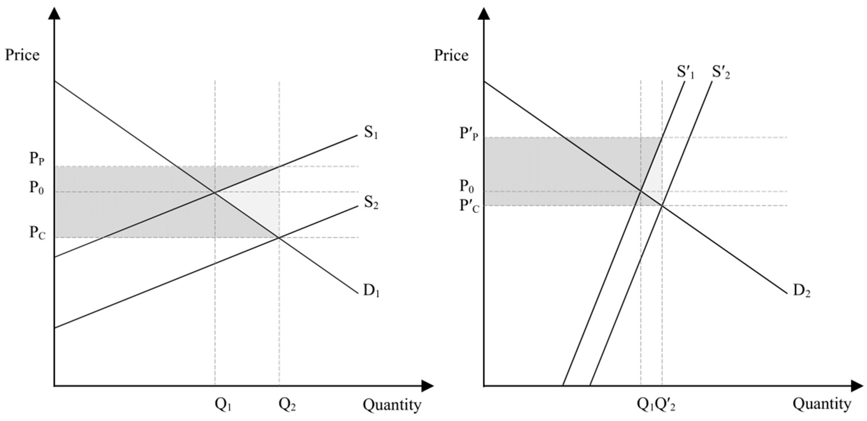Figure 2 illustrates such inefficient markets. On the left graph, S₁, D₁, Q₁, and P₀ are supply curve (marginal cost), demand curve (marginal benefit), supply quantity, and equilibrium price in the existing housing market, respectively. The introduction of a per-square-foot subsidy would create a new equilibrium, in which Q₂, P_p, and P_c are the new supply quantity, the unit price for firms, and the unit price for costumers, respectively. The right graph represents a market with a low-price elasticity of supply, in which introducing the same amount of subsidy (P_p − P_c = P′_p − P′_c) would have a little impact on supply quantity (Q′₂), while giving more benefits to producers than consumers. Similar mechanisms are in place for introducing new residential energy efficiency policies that depend on the price elasticity of demand for energy [57]. For guidance and more information, see Ref. [66].

The integration of environmental principles in an affordable housing program requires innovative policymakers to monetize and evaluate the private and public costs and benefits of the program, based on local demographic and housing market data. The extant literature suggests that certified offices and houses have higher rents and/or prices that can come from energy efficiency, water efficiency, improved air quality, and occupant productivity. Nonetheless, evaluation of public benefits (i.e., positive externalities, such as eco-system protection, and waste and carbon dioxide emission reduction) associated with green building against environmental damages caused by conventional buildings has been documented with insufficient attention and consensus in the literature [17,67]. Simulation-based life-cycle analyses have provided valuable insight into the environmental impacts of green buildings [68], but little, if any, research has been performed to date to analyze the spillover effects of green buildings, e.g., in terms of the impact of the presence or density of green buildings on prices of nearby non-green buildings. Such analyses would have provided more details on price dynamics and the social benefits of green buildings, and consequences for local sustainability and climate change policy [69]. The need for monetary analyses is reinforced by the fact that construction cost data, performance data (e.g., energy use, water use) and outcome data (e.g., on health, pollution, congestion) are generally confidential, limited, or simply unavailable, and engineering simulation studies could be hard to compare or have restricted generalizability, due to heterogeneities involved in the operation stage. Monetizing all the impacts of green affordable housing could reduce uncertainties associated with forecasts, and allow policy analysts to obtain systematic and context-driven conclusions about the social benefits of such programs, based on cost benefit analysis [70,71].

The current analysis aims to address the lack of attention in the existing literature to the residential sector in smaller urban areas, through a cost analysis of EarthCraft VA certified LIHTC developments, a price analysis of market-rate EarthCraft VA certified single-family houses, and an analysis of spillover effects associated with market-rate certified houses and affordable non-certified houses in Montgomery County, VA. As previous research [50,51,72,73,74] has documented large associations between the presence of density incentives and a higher production of green residential buildings in a state or county, we apply our findings on costs and prices to the design of a county-wide voluntary density incentive program, to explore how much additional floor area could compensate local builders for investment in the construction of green affordable housing units in for-sale and for-rent scenarios.

3. Methodology

Overview of Study Context and Datasets

This study employs two separate datasets, along with the corresponding regression analyses of construction costs and transaction prices of green affordable housing. The first dataset includes pooled cross-sectional LIHTC construction cost data from all publicly available applications on the Virginia Housing Development Authority website, as of October 2019. The cost premium sample includes 422 new construction and rehabilitation residential projects across VA, with Gold and Platinum levels of EarthCraft certification. The second dataset includes pooled cross-sectional MLS transaction data for housing units in Montgomery County, VA, between 2000 and 2019, which were used to estimate price premiums and the spillover effects of EarthCraft VA certified houses. The authors employed time-, site-, and district-specific fixed effects to capture temporal and locational changes in closed/transaction prices. We removed units built before 1800 and units with above 100 acre lots as outliers. The price premium sample includes 38 EarthCraft certified houses built between 2008 and 2019, with an average transaction price of $441,779.8 (SD 131,065), and 45 affordable rental apartment complexes. The affordable properties included Section-8 rental housing assistance apartments, apartments that accepted housing vouchers, and income-restricted complexes. The certified houses and affordable properties were in census blocks, in which 1098 and 2199 transactions took place during the study period, and located in different areas within the county, thus exhibiting no spatial autocorrelation or clustering impacts. Latitude and longitude data were obtained from Texas A&M Geo-Services website, to control for zoning characteristics and potential externalities. Data on population, education, and income at the Census-defined block group level were obtained from the US Census Bureau’s 2018 ACS 5-year estimates.

We used STATA 14 to perform hedonic regression analyses, to assess the total construction cost and transaction price impacts of EarthCraft VA certification, and to estimate the spillover effects of EarthCraft VA certified homes and affordable housing properties on non-green houses in Census-defined blocks. The hedonic approach to sale price reflects both supply and demand influences and recognizes the value of a house as an additive function of the utility-bearing characteristics of the structure, the lot, and the neighborhood in which the house is located [75]. Based on the theory of hedonic prices formulated by Ref. [76], Equation (1) is one of the earliest and most frequently used applications of linear hedonic regression models in housing offered by Ref. [77], where $v_i$ is the house value and $S_i$, $L_i$, and $N_i$ are vectors of characteristics of the structure, lot, and neighborhood, and $\alpha$,$\beta$, and $\gamma$ are vectors of unknown coefficients. Virtually all previous studies on green building price premiums used similar multivariate log–linear (i.e., semi-log) hedonic models, with time and location as fixed effects [8,29,78,79]. For the purpose of this study, Equation (1) could be re-written as Equation (2), where $G_i$ is a binary variable used to obtain the price premium of having an EarthCraft VA certification, $Y_m$ and $M_n$ denote the fixed effect of the year and the month of transaction, $C$ is a constant term, and $\eta$, $\delta$, and $\theta$ are coefficients.

$$ln{v}_i=S_i\alpha +L_i\beta +N_i\gamma +{\overline{ℰ}}_i$$

(1)

$$ln{v}_i=G_i{\eta }_i+{\displaystyle \sum }_{j=1}^5{S}_j{\alpha }_j+{\displaystyle \sum }_{k=1}^{16}{L}_k{\beta }_k+{\displaystyle \sum }_{l=1}^{16}{N}_l{\gamma }_l+{\displaystyle \sum }_{m=1}^{19}{Y}_m{\delta }_m+{\displaystyle \sum }_{n=1}^{12}{M}_n{\theta }_n+C+{\overline{\mathcal{E}}}_i$$

(2)

To obtain estimates for a voluntary density incentive program for green affordable housing in Montgomery County, VA we assumed that there are 3%, 6%, and 10% increases in construction costs associated with EarthCraft VA Certified, Gold, and Platinum levels of certification, based on a synthesis of the literature, EarthCraft industry reports, and our regression analyses. To estimate the amount of additional floor area required to incentivize green building in the for-sale scenario, we set the estimated total sale profit from new construction (i.e., market price minus the total cost of financing and production, including general contractor’s overhead and profit) under the density incentive zoning ordinance, equal to the estimated total profit from new construction under the existing zoning ordinance, and solved for the increased floor area under the density incentive zoning ordinance. Green building area (Q_g) can be estimated using Equation (3), where C and C_g are production and financing costs, and Q and Q_g are the total areas of non-green and green buildings, respectively, and P is the sale price of non-green buildings. Similarly, the incentivized affordable housing floor area is estimated using Equation (4), where P_m and P_a are sale prices, and Q_m and Q_a are the total areas of market-rate and affordable rate units, respectively. To solve for the necessary increase in density, Q_a is treated as a percentage of Q_m. In this equation, C_e and C_i are production and financing costs of building under existing zoning and under incentive conditions, respectively, and Q_e is the total area under existing zoning conditions. Alternatively, the total loss of a building’s operating income, due to the presence of rent caps on affordable units, can be considered as a per unit area additional cost of construction. In a for-rent affordable housing scenario, the net monthly operating income is equal to the constant monthly construction loan due (A), which is found by the amortization calculator formula (Equation (5)), using the total cost of construction loan (P), monthly interest rate (r), and total number of payments (n). When there is a deficit in the net monthly operating income as the result of rent caps on affordable units (often determined based on 30% of household income), the net present value of the total deficit plus the green premium, if present, is translated into a percentage of the net monthly operating income to determine the density incentive.

$$\begin{gathered} (P-C)\times Q=\left(P-C_g\right)\times Q_g\mathrm{or} \\ {Q}_g=\frac{\left(P-C\right)\times Q}{\left(P-C_g\right)} \end{gathered}$$

(3)

$$(P_m-C_e)\times Q_e=\left(P_m\times Q_m+P_a\times Q_a\right)-C_i\times \left(Q_m+Q_a\right)$$

(4)

$$A=P\frac{r{\left(1+r\right)}^n}{{\left(1+r\right)}^n-1}$$

(5)

Table 1. Description of variables in construction cost models (n = 230).

Variable	Definition	Mean	Std. Dev.	Min	Max
Continuous
Buildings	Number of buildings in a project	3.913	4.889	1	30
Cost	Total residential space construction cost in USD	11,100,000	6,876,547	2,804,831	51,300,000
Latitude	Geographical latitude of project city in decimal units	37.699	0.775	36.600	39.770
Ln_Cost	Natural logarithm of residential space construction cost	16.077	0.516	14.847	17.752
Longitude	Geographical longitude of project city in decimal units	−7.289	1.067	−86.160	−75.820
Residential Area	Total air-conditioned residential space area in square foot (SF)	77,720	36,982	21,846	262,648
Stories	Number of building stories	3.367	1.459	1	12
Year	Project year	2015.191	2.488	2011	2019
Binary
Gold Level	If building has Gold Level EarthCraft certification (1)	0.387	0.488
Platinum Level	If building has Platinum Level EarthCraft certification (1)	0.613	0.488

and

Table 2. Description of variables in transaction price models (n = 11,016).

Variable	Definition	Mean	Std. Dev.	Min	Max
Continuous
Acreage	Total lot area in acres	1.342	4.368	0.01	100
Area	Total finished interior space area in SF	2074.060	849.932	100	6696
Education	Percent 25+ adults with bachelor’s degree or higher in BG	50.394	22.626	5.982	100
Full Baths	Total number of full bathrooms	2.172	0.722	0	6
Half Baths	Total number of half bathrooms	0.482	0.546	0	6
Income	Median household income in BG in 2017 in 1000 USD	70.866	26.453	6.86	141.25
Latitude	Geographical latitude of lot in decimal units	37.177	0.060	36.994	37.348
Ln_Price	Natural logarithm of the total house price	12.215	0.516	8.700	13.805
Longitude	Geographical longitude of lot in decimal units	−80.415	0.049	−80.611	−80.188
Month	Transaction month fixed effects	6.516	2.982	1	12
Population	Total population living in BG in 100 persons in 2017	19.271	6.339	5.29	33.51
Price	Total house price in USD	228,435.800	115,920.100	6000	990,000
Year	Transaction year fixed effects	2010.935	5.155	2001	2019
Year Built	Year of construction	1985.561	23.454	1800	2019
Binary
Christiansburg	If building is in Christiansburg (1)	0.394	0.489
EarthCraft	If building is EarthCraft certified (1)	0.003	0.055
EnergyStar	If building is EnergyStar certified (1)	0.001	0.037
Montgomery	If building is in Montgomery (1)	0.324	0.468
Public Transport	If public transport is within walkable distance (1)	0.088	0.283
Recreation	If recreational facility is within walkable distance (1)	0.050	0.217
School	If elementary school is within walkable distance (1)	0.078	0.268
Townhouse	If building is a townhouse (1)	0.127	0.333

include descriptive statistics of the sample set and descriptions of primary independent variables used in the current analysis. In addition to these variables, price estimate models accounted for the fixed effects of years of transaction (19 variables), site characteristics (16 variables), and neighborhood characteristics (16 variables). As opposed to single-family and multi-family developments, planned residential developments (PRDs) often achieve multiple incentives (e.g., flexible unit sizes, increased FARs, and decreased minimum lot sizes, and multiple community features) and, thus, should be studied on a case-by-case basis, for the purpose of allocating density incentives (see Ref. [80]). Third-party consultants should examine the accuracy of pro-forma statements of PRD builders, and the minimum profitable production costs and land costs can be obtained from RSMeans and linear regression of land price on land characteristics (see, e.g., Ref. [81]). Detailed sale price estimates can be obtained from MLS data using hedonic regression—or other advanced multivariate analytical tools—that accounts for the variety of unit characteristics. Once the difference between the estimated total costs and sale prices are determined, planners could negotiate with the builder on the project’s expected benefits for the society, based on the magnitude of the estimated profit.

4. Results

4.1. Construction Cost Premiums

The LIHTC properties data suggest that the level of ‘greenness’ of LIHTC buildings has become increasingly important, as opposed to simply obtaining the ‘barely green’ (i.e., EarthCraft VA Certified) certification.

Table 3. Ordinary least squares (OLS) regression analyses of residential construction cost.

Variable	All		New Construction		Rehabilitation
	Coef.	R.S.E.	Coef.	R.S.E.	Coef.	R.S.E.
Platinum Level	0.0849 **	0.0406	0.0450	0.0521	0.1187 **	0.0610
Rehabilitation	−0.4941 ***	0.0400
Age					0.0041 ***	0.0012
Buildings	0.0106 ***	0.0032	0.0094 **	0.0036
Residential Area	1.07 × 10−5 ***	6.55 × 10−7	8.42 × 10−6 ***	7.02 × 10−7	1.42 × 10−5 ***	7.85 × 10−7
Stories	0.1252 ***	0.0177	0.0977 ***	0.0217	0.1007 ***	0.0210
Latitude	0.1128 ***	0.0229	0.1908 ***	0.0300	0.0252	0.0391
Longitude	0.0199	0.0102	0.0505 ***	0.0211	0.0232	0.0121
Year	0.0571 ***	0.0078	0.0466 ***	0.0101	0.0690 ***	0.0110
Constant	−102.9944 ***	15.8505	−82.1426 ***	20.5282	−124.1019 ***	22.1574
Obs	422		230		191
Prob > F	0.000		0.000		0.000
R-squared	0.857		0.790		0.800
Adj R-squared	0.854		0.783		0.792
Root MSE	0.292		0.240		0.296

Notes:1. The dependent variable is the natural log of the total cost. 2. The reference level of EarthCraft certification for which the dummy variable is zero, is EarthCraft Gold. 3. *** and ** denote p < 0.01 and p < 0.05, respectively.

presents results from the regression analysis of the total construction cost of LIHTC residential projects with Gold and Platinum levels of EarthCraft certification. To interpret the percentage change in construction cost in these semi-log models, where the dependent variable has been log-transformed but the predictors have not, we exponentiate the coefficient of the independent variable, subtract one from the result, and multiply it by one hundred to interpret coefficients in percentages. The first model (All) includes both new construction and rehabilitation projects and indicates a significant cost impact of change in the level of certification. Nonetheless, the other models distinguish new construction and rehabilitation project data, respectively, suggesting that a change of certification level does increase the average cost of new constructions (4.60%, p = 0.368) but the increase is statistically insignificant. Model 2 suggests that the change has a considerable impact on the total cost of rehabilitation, and the impact is statistically significant (12.60%, p = 0.033). The 95% confidence intervals for new construction and rehabilitation impacts based on Robust Standard Errors (R.S.E.) are −5.94–15.91% and −0.16–26.99%, respectively. Variance Inflation Factor (VIF) of the variables and models are presented in the Appendix A.

4.2. Price Premiums and Spillover Effects

Table 4. OLS regression analyses of single-family house prices.

Variable	Model-1		Model-2		Model-3
	Coef.	R.S.E.	Coef.	R.S.E.	Coef.	R.S.E.
EarthCraft	0.1403 ***	0.0282	0.1568 ***	0.0260	0.1691 ***	0.0288
EnergyStar	0.0565	0.0425	0.0725 **	0.0362	0.0475	0.0380
Area	0.0003 ***	0.0000	0.0003 ***	0.0000	0.0003 ***	0.0000
Full Baths	0.0534 ***	0.0056	0.0487 ***	0.0055	0.0534 ***	0.0056
Half Baths	0.0666 ***	0.0051	0.0662 ***	0.0050	0.0697 ***	0.0051
Townhouse	−0.1493 ***	0.0066	−0.1589 ***	0.0065	−0.1487 ***	0.0067
Year Built	0.0047 ***	0.0002	0.0047 ***	0.0002	0.0046 ***	0.0002
Acreage	0.0094 ***	0.0013	0.0094 ***	0.0013	0.0093 ***	0.0013
Latitude	0.2055	0.1513	−0.1308	0.1561	0.1431	0.1549
Longitude	−0.4008 ***	0.1225	−0.1932	0.1244	−0.4624 ***	0.1239
Public Transport	−0.0265 ***	0.0076	−0.0190 **	0.0075	−0.0131	0.0081
Recreation	0.0183	0.0098	0.0104	0.0097	0.0178	0.0101
School	0.0474 ***	0.0082	0.0280 ***	0.0083	0.0458 ***	0.0083
Christiansburg	−0.0438 ***	0.0150	−0.0194	0.0151	−0.0474 ***	0.0152
Montgomery	−0.0671 ***	0.0100	−0.0216 **	0.0103	−0.0662 ***	0.0102
Education			0.0032 ***	0.0002
Income					0.0011 ***	0.0001
Population			−0.0011 **	0.0005	−0.0015 ***	0.005
Year FE	Yes		Yes		Yes
Month FE	Yes		Yes		Yes
Site FE	Yes		Yes		Yes
District FE	Yes		Yes		Yes
Obs	11,016		10,996		10,773
Adj R-squared	0.746		0.752		0.748
Root MSE	0.261		0.258		0.261

Notes: 1. The dependent variable is the natural log of transaction price. 2. *** and ** denote p < 0.01 and p < 0.05, respectively. 3. FE refers to fixed effects.

presents results from the regression analysis of single-family houses with and without EarthCraft VA certification. Based on Model 1, which includes the hedonic characteristics of houses, lots, and neighborhoods, EarthCraft VA certified homes are, on average, associated with a 15.06% sale price premium compared to otherwise identical buildings, and the premium is statistically significant. Houses with EnergyStar appliances are, on average, associated with a 5.81% sale price premium compared to houses without those features, but the premium is statistically insignificant. Model 2 and Model 3 control for the socioeconomic (SES) variables of education, income, and population at the Census-defined block group level, the smallest geographical level for which these data are available. Although these SES variables show small coefficients, the inclusion of these statistically significant variables increases the estimated average sale price premium for EarthCraft VA certified homes from 15.06% to 16.98% and 18.42%. The models also suggest that houses located within walking distance of public transport on MLS records are negatively affected by some undesirable locational characteristics (e.g., air pollution, congestion, noise) and, on average, are 2.69% less valuable. Nonetheless, houses located within walking distance of elementary schools are transacted with an average of 4.85% sale price premiums, compared to similar houses not located within walking distance of the district elementary school.

Table 5. Analyses of spillover effects of certified houses and non-certified affordable houses.

Variable	Model-1		Model-2		Model-3
	Coef.	R.S.E.	Coef.	R.S.E.	Coef.	R.S.E.
Green building	0.0566 ***	0.0067	0.0447 ***	0.0066	0.0662 ***	0.0070
Affordable housing	−0.0072	0.0058	0.0037	0.0058	−0.0029	0.0059
Area	0.0003 ***	0.0000	0.0003 ***	0.0000	0.0003 ***	0.0000
Full Baths	0.0547 ***	0.0056	0.0507 ***	0.0055	0.0551 ***	0.0056
Half Baths	0.0674 ***	0.0051	0.0667 ***	0.0050	0.0713 ***	0.0051
Townhouse	−0.1430 ***	0.0067	−0.1526 ***	0.0067	−0.1425 ***	0.0068
Year Built	0.0046 ***	0.0002	0.0046 ***	0.0002	0.0046 ***	0.0002
Acreage	0.0094 ***	0.0013	0.0094 ***	0.0013	0.0093 ***	0.0013
Latitude	0.2300	0.1519	−0.1143	0.1566	0.1743	0.1552
Longitude	−0.3894 ***	0.1228	−0.1941	0.1243	−0.4509 ***	0.1238
Public Transport	−0.0301 ***	0.0076	−0.0221 ***	0.0075	−0.0159	0.0081
Recreation	0.0176	0.0098	0.0102	0.0097	0.0168	0.0101
School	0.0497 ***	0.0082	0.0298 ***	0.0083	0.0474 ***	0.0083
Christiansburg	−0.0429 ***	0.0151	−0.0186	0.0151	−0.0454 **	0.0152
Montgomery	−0.0623 ***	0.0100	−0.0172	0.0103	−0.0594 ***	0.0101
Education			0.0032 ***	0.0002
Income					0.0011 ***	0.0001
Population			−0.0011 **	0.0005	−0.0017 ***	0.0005
Year FE	Yes		Yes		Yes
Month FE	Yes		Yes		Yes
Site FE	Yes		Yes		Yes
District FE	Yes		Yes		Yes
Obs	10,975		10,975		10,741
Adj R-squared	0.745		0.751		0.748
Root MSE	0.261		0.258		0.261

Notes: *** and ** denote p < 0.01 and p < 0.05.

presents results from the regression analysis of spillover effects of certified market-rate and non-certified affordable housing units on other houses within the Census-defined block. Based on Model-1, which includes hedonic characteristics of houses, lots, and neighborhoods, the presence of certified units in a block is, on average, associated with a 5.82% sale price premium for non-certified houses within the block (the 95% confidence interval is 4.43–7.23%), and the spillover effect is statistically significant at 99%. The presence of non-certified affordable housing units is associated with an average of −0.72% sale price premiums for non-certified houses within the block (the 95% confidence interval is −1.88–0.42%), but the spillover effect is statistically insignificant. Model 2 and Model 3 control for the socioeconomic variables of education, income, and population at the block group level, and show slight changes, but statistically significant spillover effects.

Table 6. Analyses of spillover effects of certified houses and non-certified affordable houses.

	2004–2007		2008–2011		2012–2015		2016–2018
	Coef.	R.S.E.	Coef.	R.S.E.	Coef.	R.S.E.	Coef.	R.S.E.
Green building present	0.0275 **	0.0137	0.0371 **	0.0188	0.0573 ***	0.0133	0.0781 ***	0.0130
Affordable housing present	−0.0197 *	0.0104	−0.0138	0.0152	0.0073	0.0121	−0.0061	0.0120
Area	0.0003 ***	0.0000	0.0003 ***	0.0000	0.0003 ***	0.0000	0.0003 ***	0.0000
Full Baths	0.0592 ***	0.0100	0.0717 ***	0.0138	0.0540 ***	0.0118	0.0527 ***	0.0120
Half Baths	0.0723 ***	0.0087	0.0783 ***	0.0130	0.0662 ***	0.0113	0.0556 ***	0.0103
Townhouse	−0.1196 ***	0.0129	−0.1263 ***	0.0156	−0.1714 ***	0.0135	−0.1732 ***	0.0128
Year Built	0.0038 ***	0.0003	0.0045 ***	0.0005	0.0052 ***	0.0004	0.0050 ***	0.0004
Acreage	0.0106 ***	0.0025	0.0183 ***	0.0037	0.0110 ***	0.0020	0.0080 ***	0.0019
Latitude	0.2981	0.2395	0.5963	0.4335	0.5681	0.4052	−0.8080 **	0.3959
Longitude	−0.6974 ***	0.1801	−0.3204	0.3291	−0.0799	0.3157	−0.1861	0.3378
Christiansburg	−0.0092	0.0299	−0.0623	0.0432	−0.0771 **	0.0338	−0.0232	0.0289
Montgomery	−0.0478 ***	0.0186	−0.0543 **	0.0273	−0.1112	0.0220	−0.0589 ***	0.0198
Year FE	Yes		Yes		Yes		Yes
Month FE	Yes		Yes		Yes		Yes
Site FE	Yes		Yes		Yes		Yes
District FE	Yes		Yes		Yes		Yes
Obs	2972		1887		2494		2700
Adj R-squared	0.781		0.736		0.745		0.730
Root MSE	0.219		0.275		0.268		0.278

Notes: *** and ** denote p < 0.01 and p < 0.05.

presents a similar analysis of spillover effects in four different historical periods. The first EarthCraft VA certified houses in Montgomery County, VA, were built in 2008. Therefore, Model 1 to Model 4 suggest that: (1) blocks in which market-rate certified houses were built in 2008 were relatively more valuable than other blocks in the county; (2) the value premium of those blocks in which market-rate certified houses were built in 2008 and later, has continuously increased over time. During the study period, the presence of affordable housing units was associated with negligible spillover effects, which were often statistically insignificant.

4.3. Density Incentive Calculations

Table 7. Estimates of incentives for green single-family and multi-family housing.

	Area (sqft)	Price/Rent	Cost of Construction				Incentive Floor Area
	Non-Green	Non-Green	Non-Green	Certified	Gold	Platinum	Certified	Gold	Platinum
Single-Family	1200	$199	$135	$139	$143	$149	6.85%	14.71%	27.18%
(For sale)	1400	$180	$128	$132	$136	$141	8.06%	17.54%	33.09%
	1600	$176	$123	$127	$131	$136	7.62%	16.50%	30.89%
	1800	$165	$118	$122	$126	$130	8.27%	18.04%	34.18%
	2000	$157	$113	$117	$120	$125	8.45%	18.45%	35.06%
	2200	$151	$110	$113	$116	$121	8.74%	19.16%	36.61%
Multi-Family	50,000	$204	$106	$109	$112	$117	3.44%	7.25%	13.03%
Low-rise	60,000	$204	$96	$99	$102	$106	2.82%	5.90%	10.49%
(For sale)	70,000	$204	$89	$92	$95	$99	2.47%	5.15%	9.12%
	80,000	$204	$85	$88	$91	$94	2.26%	4.71%	8.30%
	90,000	$204	$82	$85	$88	$91	2.14%	4.43%	7.80%
	100,000	$204	$81	$83	$86	$89	2.06%	4.27%	7.51%
Multi-Family	50,000	$0.96	$106	$109	$112	$117	3.09%	6.28%	10.71%
Low-rise	60,000	$0.84	$96	$99	$102	$106	3.09%	6.28%	10.71%
(For rent)	70,000	$0.76	$89	$92	$95	$99	3.09%	6.28%	10.71%
	80,000	$0.71	$85	$88	$91	$94	3.09%	6.28%	10.71%
	90,000	$0.67	$82	$85	$88	$91	3.09%	6.28%	10.71%
	100,000	$0.65	$81	$83	$86	$89	3.09%	6.28%	10.71%

presents the results of our density incentive estimates for single-family and multi-family housing of various sizes in for-sale and for-rent scenarios, respectively, where costs and prices are shown in per square foot of residential area. In the for-sale scenario, builders recover cost premiums at sale times, whereas, in the for-rent scenario, cost premiums are recovered in the long run. In the for-rent scenario, the amount of incentive, i.e., the percentage of additional floor area, to compensate builders, is proportional to, and slightly higher than, the green building certification cost premium expressed in percentage.

Table 8. Estimates of incentives for green affordable housing in a for-rent low-rise scenario.

Units	Area Median Income	Count	Area (sqft)	Market Rent/Unit	Affordable Rent/Unit	Market Income	Loss of Income
0-Bedroom	30%	10	500	$750	$276	$7500	$4744
500 sqft	50%	10	500	$750	$458	$7500	$2916
1 person max	80%	10	500	$750	$733	$7500	$169
	100%	5	500	$750	-	$3750	$0
	120%	5	500	$750	-	$3750	$0
	Market	4	500	$750	-	$3000	$0
1-Bedroom	30%	10	750	$960	$368	$9600	$5925
750 sqft	50%	10	750	$960	$611	$9600	$3488
1.5 person max	80%	10	750	$960	-	$9600	$0
	100%	5	750	$960	-	$4800	$0
	120%	5	750	$960	-	$4800	$0
	Market	4	750	$960	-	$3840	$0
2-Bedroom	30%	10	1000	$1230	$471	$12,300	$7588
1000 sqft	50%	10	1000	$1230	$655	$12,300	$5750
Three persons max	80%	10	1000	$1230	$1,048	$12,300	$1825
	100%	5	1000	$1230	-	$6150	$0
	120%	5	1000	$1230	-	$6150	$0
	Market	5	1000	$1230	-	$6150	$0
Total			100,000			$130,590	$32,403
Loss of Income/Market Income Ratio (24.81%)
Area after incentive (add the Ratio)	124,813
Area after EarthCraft Certified (add 3.09%)	128,669
Area after EarthCraft Gold (add 6.28%)	132,651
Area after EarthCraft Platinum (add 10.71%)	138,180

presents an example of a 100,000 sqft low-rise multifamily building, in which about 25% of the total market-based rent is lost, due to the presence of affordable housing units, dedicated to local workforce with different levels of income relative to the area median income. In this case, an increase in the residential area to 124,813 sqft could recover the loss in rent, and further increases to 128,669 sqft, 132,651 sqft, and 138,180 sqft are enough to recover the total construction cost of different levels of EarthCraft VA certification during the operation of the building. The calculations are based on a 15-year construction loan with a 5% interest rate.

5. Discussion

5.1. Key Findings and Comparison to Previous Work

Based on an analysis of 422 LIHTC projects that applied for income tax credits between 2011 and 2019 across VA, our findings suggest that an increase in the level of EarthCraft certification, from Gold to Platinum, increases the cost of rehabilitation and new construction by 12.60% and 4.60%, on average, while controlling specifically for statistically significant attributes of the residential area, number of stories, age of existing buildings, coordinates, and the year of construction. The result of the cost premium on new construction is supported by Ref. [8], as small increases in the level of green building certification of new constructions have statistically insignificant cost impacts. However, similar increases in the level of certification in rehabilitation are associated with large and significant cost premiums. A potential reason for this cost premium is the impact of green building criteria on building enclosures, which typically constitute a large part of rehabilitation projects. Compared to new construction projects, rehabilitation projects might be more cost-effective in terms of rate-of-return, but rehabilitation project options and specifications might require additional scope and/or restrict the menu of credit-earning solutions that would be available in new constructions. Another complicating factor is that, within green building programs, there are separate certifications for the rehabilitation of existing buildings, whereas almost all research to date has focused on new construction cost premiums. Whether new construction or rehabilitation, buildings certified as green within each category are likely to take longer to complete than conventional buildings, thus requiring less experienced builders to wait longer to obtain revenues. Allocating more incentives to rehabilitation projects could be reasonable where there is a tendency to lower undesirable economic, environmental, and social impacts of developments (e.g., reduced cost and time of construction, reduced waste generation and resource consumption, increased reuse of existing materials), thus increasing social benefits [82,83].

Houses certified under the EarthCraft VA program in Montgomery County, VA are associated with significant sale price premiums, with an estimated average of 15.06%, of which about 2.79% could be attributed to locational characteristics (based on Table 6) that were not captured. Therefore, the 12.27% premium translates to a dollar value of about $32,105, considering the average home sale price for the county, of $261,660 in 2018. This finding is in general agreement with a previous study that found an increase of 8.30% associated with 300 EarthCraft certified houses from a sample of 1094 homes sold in Atlanta, GA between 2007 and 2010, which could be lesser, due to a recession in the housing market [30]. In addition, Ref. [29] found 8–9% premiums associated with housing units with local certification schemes in Austin, TX after matching and hedonic analyses. The relatively higher price premium in this study could be partially attributed to a higher potential for savings from energy efficiency in the context of Montgomery, VA, compared to Atlanta, GA or Austin, TX. Anecdotally, EarthCraft VA reports an upfront cost premium of 0.5–3% based on local builders, suggesting that the capitalization of green building features into transaction prices, on average, substantially exceeds upfront cost premiums. In the current study, the impact of EnergyStar certification on housing unit prices is smaller (around 5.81%) and not always statistically significant.

The density bonus estimates suggest that, to recover 3%, 6%, and 10% incremental cost premiums associated with for-sale single-family houses in Blacksburg, VA, homebuilders need about 5–10%, 10–20%, and 25–40% increases in floor area, respectively. More precise estimates can be achieved based on the structural and locational characteristics of individual buildings (Table 7). Nonetheless, housing prices are also confounded by dynamic market-driven factors, making it difficult to forecast housing prices using conventional methods. It is likely that regulatory and technological reforms affect certification costs and willingness to invest in certified buildings. Factors such as builders’ capacity and experience in green building, the energy literacy of households, availability of professional training programs and financial solutions, and recognition of green buildings in the market, are important to the economic viability of green buildings. It is also likely that local opposition to affordable housing causes construction delays, delays in leasing or selling units, etc. Therefore, such thresholds could provide local planners with some level of flexibility in decision-making. In for-sale, low-rise and mid-rise multi-family buildings, the percentage and variability of density incentives decrease. In general, our results indicate that where housing is expensive relative to its basic costs of production (e.g., due to zoning) small increases in building area could help builders recoup their initial investment in green affordable housing, while keeping the price per unit area unchanged for home buyers and renters. Planners could strategically allocate density incentives towards meeting other goals set by local comprehensive plans or zoning codes, e.g., promoting socio-economically balanced communities, but need to ensure that other constraints, e.g., water permits and height limits, are not limiting development [84]. The real test of whether the offered density incentive ordinance offsets the costs of green certification and price/rent limits is if local builders would prefer them over the existing ordinance [36]. Further incentives might include the use of economic instruments (e.g., tax reduction, financial assistance) or the relaxation of zoning requirements (e.g., lot coverage, parking, public space, allowing for off-site construction of affordable units) [85].

Non-certified market-rate houses in proximity to EarthCraft VA certified houses have been associated with increasing sale price premiums of 3.78%, 5.90%, and 8.12%, according to the three recent models specified in Table 6. Assuming about 2.79% of the associated premium belongs to unknown locational characteristics (from 2004–2007 model in Table 6), the remaining 5.33% premium in the period 2016–2018 would equate to a dollar value of $13,946 when considering the average home sale price for the county of $261,660 in 2018. The spillover effect has increased in the last few years. The combination of price premium (private benefit) and spillover effect (public benefit), which together represents the social benefits of green building in the county, is much higher than the average cost premium of obtaining green building certification, and justifies the local government’s investment in an integrated green affordable housing program. The program could reduce public spending, resulting from disproportionate costs of energy, transport, healthcare, safety, etc., on low-income groups. As the clustering of green buildings could also disproportionately impact housing affordability by increasing local property values, the introduction of affordable housing units could also address potential segregation impacts. We find evidence that houses in proximity to schools have higher prices, a finding that is supported by the hedonic price literature on pedestrian-and transit-oriented development [86]. Nonetheless, we find negative price effects associated with proximity to public transportation, which could be explained by the fact that the public transportation system in the county is primarily designed to service student riders, and more expensive houses tend to be in less congested areas.

Extant research on the spillover effects of affordable housing and LIHTC properties has found that the magnitude of effects depends on a variety of factors, including but not limited to, type and implementation of housing programs, design and management of properties, characteristics of host neighborhoods, and concentration of affordable housing [37,40]. The literature recognizes several reasons for local opposition to any new—and even expensive —housing units, including concerns about the character and quality of structures, negative externalities, diminishing valued open space, etc., which might contribute to a decline in property values [87,88]. In Montgomery County, VA, non-certified housing units that co-exist with affordable housing developments in a Census block demonstrate an average sale price premium of −0.72%, which is statistically insignificant. The presence of positive spillover effects associated with certified units suggests that the integration of green building with affordable housing—along with the dispersal of affordable housing throughout the city, reducing the concentration of poverty in buildings through mixed-income developments, and quality management of affordable properties—could enhance the attractiveness of affordable properties in host neighborhoods and reduce local opposition to government-assisted housing.

5.2. Recommendations for Future Research

Our results show that large and significant cost impacts are associated with small increases in the level of certification in rehabilitation projects. Therefore, future research should further investigate the impact of green building certifications on rehabilitation projects, as there is currently no comparable systematic study available in the literature. Existing buildings before new energy code improvements of the late 2000s are our largest current stock. As green building policies are increasingly adopted by local governments, multi-jurisdictional studies with larger sample sizes are needed to draw firm conclusions on the external impacts of both market-rate and affordable green housing units, e.g., on local economic, environmental, and social sustainability rates [89]. In this research, we examined such effects, based on either the presence or absence of such units, due to sample size limitations, but it would be more fruitful if the relationship is explored in terms of the proportion of land devoted to, and distance from, certified units and affordable units over time.

Our sample set represents all MLS transactions in the county during the last twenty years. However, the analysis in this case-study is restricted, due to the slow diffusion of green building practices in the local marketplace not allowing for further statistical analyses, e.g., propensity score weighting and matching to reduce selection bias. Despite constant increases in the frequency of transactions in the local market since 2008, and the capitalization of green certifications into house prices, the number of certified houses has not increased since 2014. Such declines, which might be attributed to the emergence of stricter energy-efficiency codes, improvements in construction standards, cost of housing, or negative sentiments towards green buildings in the real estate industry, is worth further investigation in the future research [78].

A common limitation in the study of green building cost premium is the lack of organized construction data. LIHTC projects are subject to the Freedom of Information Act (FOIA), which provides the public with access to federal agency records, providing useful resources for future research on the construction costs of multi-family residential buildings. Nonetheless, most LIHTC agencies in the region did not start to organize and make construction project data electronically available until recent years. In fact, the Virginia Housing Development Authority (VHDA) had the only organized, publicly accessible archive of LIHTC construction data in the region, which itself was limited to recent projects. The availability of more LIHTC data in the future would provide researchers with opportunities to investigate the social impacts of green affordable housing, a more detailed assessment of which could help address existing barriers, and enhance the market recognition of green and affordable housing [90].

6. Conclusions

This empirical study explored density bonus options for green affordable housing, by analyzing construction costs, sale prices, and spillover effects for green certifications and affordable housing units.

Table 9. Summary of results from the past research and the present study.

Extant Literature Results

Study Results

1) Previous research has often focused on the capitalization of nationally recognized labels into commercial property prices in larger cities. 2) There is little evidence on the magnitude of upfront green construction cost premiums in the residential sector in the US. 3) A general conclusion from the past analyses is that green buildings can have small upfront cost premiums, but price premiums often offset the cost of certification. 4) Previous research suggests well-maintained affordable housing properties can appreciate property values in neighborhoods containing deteriorating housing units 5) Integration of environmental principles in affordable housing requires cost and benefit analyses based on local demographic and housing market data.

1) Obtaining a green certification increases the cost of new housing projects, but the increase is not statistically significant. 2) Obtaining a green certification has a large impact on the cost of rehabilitation projects, and the impact is statistically significant. 3) The value premium of blocks in which market-rate certified houses are built has continuously increased over time. 4) The presence of non-green affordable housing units is associated with negligible spillover effects, which are often statistically insignificant. 5) Small density incentives help builders recoup their initial investment in green building in areas where housing is expensive

summarizes the results from the past research and the present study. Our findings indicate that: (1) the supply of green rehabilitation projects requires more incentives than the supply of new construction projects with identical certification levels, and policymakers should account for these differences when designing incentive programs (2) the integration of green and affordable units is economically justified and socially beneficial, since both private owners and the public can enjoy its positive economic, environmental, and equity impacts (3) green and affordable housing initiatives could have a positive price impact on peer buildings and reduce the risk of investment in affordable housing, by enhancing neighborhood conditions and competition on sustainability metrics (4) Small voluntary density incentives could help facilitate the integration of green building with affordable housing, to promote multiple sustainable development goals, where housing is expensive relative to its basic costs of production. Achieving green building compliance through third-party verification programs—rather than government-designed programs—could facilitate sustainable development by reducing the cost of program administration. Since buildings represent about 40% of global energy use, and 30% of global greenhouse gas emissions, the major source of contributions to climate change, there are considerable opportunities for positive large-scale impacts on global sustainability and climate change mitigation by gradual investment in the environmental sustainability of local housing markets and, at the same time, opportunities to address housing affordability and environmental justice [91].

References

1. USDOE. Use of Energy in the United States. Available online: https://www.eia.gov/energyexplained/index.php?page=us_energy_use (accessed on 28 July 2019).
2. Glaeser, E.L.; Gyourko, J. The impact of building restrictions on housing affordability. Econ. Policy Rev. 2003, 9, 1–19. [Google Scholar]
3. Adelle, C.; Russel, D. Climate policy integration: a case of déjà vu? Environ. Policy Gov. 2013, 23, 1–12. [Google Scholar] [CrossRef]
4. Jordan, A.; Lenschow, A. Environmental policy integration: a state of the art review. Environ. Policy Gov. 2010, 20, 147–158. [Google Scholar] [CrossRef]
5. Pearce, A.R.; DuBose, J.R.; Bosch, S.J. Green Building Policy Options for the Public Sector. J. Green Build. 2007, 2, 156–174. [Google Scholar] [CrossRef]
6. Zhao, D.; McCoy, A.P.; Agee, P.; Mo, Y.; Reichard, G.; Paige, F. Time effects of green buildings on energy use for low-income households: A longitudinal study in the United States. Sustain. Cities Soc. 2018, 40, 559–568. [Google Scholar] [CrossRef]
7. Fuerst, F.; Kontokosta, C.; McAllister, P. Determinants of green building adoption. Environ. Plan. B Plan. Des. 2014, 41, 551–570. [Google Scholar] [CrossRef]
8. Chegut, A.; Eichholtz, P.; Kok, N. The price of innovation: An analysis of the marginal cost of green buildings. J. Environ. Econ. Manag. 2019, 98, 102248. [Google Scholar] [CrossRef] [Green Version]
9. McCabe, M. High-Performance Buildings–Value, Messaging, Financial and Policy Mechanisms; Pacific Northwest National Lab.(PNNL): Richland, WA, USA, 2011.
10. Hu, M. Does zero energy building cost more?–An empirical comparison of the construction costs for zero energy education building in United States. Sustain. Cities Soc. 2019, 45, 324–334. [Google Scholar] [CrossRef]
11. Kahn, M.E.; Kok, N. The capitalization of green labels in the California housing market. Reg. Sci. Urban Econ. 2014, 47, 25–34. [Google Scholar] [CrossRef]
12. USGBC. An Introduction to LEED and Green Building; US Green Building Council: Washington, DC, USA, 2019. [Google Scholar]
13. EarthCraft Who is EarthCraft. Available online: https://earthcraft.org/who-is-earthcraft/ (accessed on 24 August 2019).
14. Fuerst, F. Building momentum: An analysis of investment trends in LEED and Energy Star-certified properties. J. Retail Leis. Prop. 2009, 8, 285–297. [Google Scholar] [CrossRef] [Green Version]
15. Zuo, J.; Zhao, Z.-Y. Green building research–current status and future agenda: A review. Renew. Sustain. Energy Rev. 2014, 30, 271–281. [Google Scholar] [CrossRef]
16. Dwaikat, L.N.; Ali, K.N. Green buildings cost premium: A review of empirical evidence. Energy Build. 2016, 110, 396–403. [Google Scholar] [CrossRef]
17. Zhang, L.; Wu, J.; Liu, H. Turning green into gold: A review on the economics of green buildings. J. Clean. Prod. 2018, 172, 2234–2245. [Google Scholar] [CrossRef]
18. Matthiessen, L.F.; Morris, P. Costing Green: A Comprehensive Cost Database and Budgeting Methodology; USGBC: Washington, DC, USA, 2004. [Google Scholar]
19. Matthiessen, L.F.; Morris, P. Cost of Green Revisited: Reexamining the Feasibility and Cost Impact of Sustainable Design in the Light of Increased Market Adoption; Continental Automated Buildings Association: Ottawa, ON, Canada, 2007. [Google Scholar]
20. Fischer, C.; Lyon, T.P. Competing environmental labels. J. Econ. Manag. Strategy 2014, 23, 692–716. [Google Scholar] [CrossRef]
21. Earth Craft. What is EarthCraft? Available online: https://earthcraft.org/homeowners/homeowner-faqs/ (accessed on 5 August 2019).
22. GSA. LEED Cost Study; US General Services Administration: Washington, DC, USA, 2004. Available online: https://archive.epa.gov/greenbuilding/web/pdf/gsaleed.pdf (accessed on 24 August 2019).
23. Eichholtz, P.; Kok, N.; Quigley, J.M. Doing well by doing good? Green office buildings. Am. Econ. Rev. 2010, 100, 2492–2509. [Google Scholar] [CrossRef]
24. Eichholtz, P.; Kok, N.; Quigley, J.M. The economics of green building. Rev. Econ. Stat. 2013, 95, 50–63. [Google Scholar] [CrossRef]
25. Fuerst, F.; McAllister, P. Eco-labeling in commercial office markets: Do LEED and Energy Star offices obtain multiple premiums? Ecol. Econ. 2011, 70, 1220–1230. [Google Scholar] [CrossRef]
26. Fuerst, F.; McAllister, P. Green Noise or Green Value? Measuring the Effects of Environmental Certification on Office Values. Real Estate Econ. 2011, 39, 45–69. [Google Scholar] [CrossRef]
27. Robinson, S.; McAllister, P. Heterogeneous price premiums in sustainable real estate? An investigation of the relation between value and price premiums. J. Sustain. Real Estate 2015, 7, 1–20. [Google Scholar]
28. Wiley, J.A.; Benefield, J.D.; Johnson, K.H. Green design and the market for commercial office space. J. Real Estate Finance Econ. 2010, 41, 228–243. [Google Scholar] [CrossRef]
29. Walls, M.; Gerarden, T.; Palmer, K.; Bak, X.F. Is energy efficiency capitalized into home prices? Evidence from three US cities. J. Environ. Econ. Manag. 2017, 82, 104–124. [Google Scholar] [CrossRef]
30. Stephenson, R.M. Quantifying the Effect of Green Building Certification on Housing Prices In Metropolitan Atlanta. Master’s Thesis, Georgia Institute of Technology, Atlanta, GA, USA, December 2012. [Google Scholar]
31. Koirala, B.S.; Bohara, A.K.; Berrens, R.P. Estimating the net implicit price of energy efficient building codes on US households. Energy Policy 2014, 73, 667–675. [Google Scholar] [CrossRef]
32. Robinson, S.; Simons, R.; Lee, E.; Kern, A. Demand for green buildings: Office tenants’ stated willingness-to-pay for green features. J. Real Estate Res. 2016, 38, 423–452. [Google Scholar]
33. Ezennia, I.S.; Hoskara, S.O. Methodological weaknesses in the measurement approaches and concept of housing affordability used in housing research: A qualitative study. PLoS ONE 2019, 14, e0221246. [Google Scholar]
34. HUD Glossary of HUD Terms. Available online: https://archives.huduser.gov/portal/glossary/glossary.html (accessed on 28 July 2019).
35. Quigley, J.M.; Raphael, S. Is housing unaffordable? Why isn’t it more affordable? J. Econ. Perspect. 2004, 18, 191–214. [Google Scholar] [CrossRef]
36. Powell, B.; Stringham, E. The economics of inclusionary zoning reclaimed: how effective are price controls. Fla. St. UL Rev. 2005, 33, 471. [Google Scholar]
37. Baum-Snow, N.; Marion, J. The effects of low income housing tax credit developments on neighborhoods. J. Public Econ. 2009, 93, 654–666. [Google Scholar] [CrossRef] [Green Version]
38. Johnson, M.P.; Ladd, H.F.; Ludwig, J. The benefits and costs of residential mobility programmes for the poor. Hous. Stud. 2002, 17, 125–138. [Google Scholar] [CrossRef]
39. Mueller, E.J.; Tighe, J.R. Making the case for affordable housing: Connecting housing with health and education outcomes. J. Plan. Lit. 2007, 21, 371–385. [Google Scholar] [CrossRef]
40. Nguyen, M.T. Does affordable housing detrimentally affect property values? A review of the literature. J. Plan. Lit. 2005, 20, 15–26. [Google Scholar] [CrossRef]
41. Santiago, A.M.; Galster, G.C.; Tatian, P. Assessing the property value impacts of the dispersed subsidy housing program in Denver. J. Policy Anal. Manag. J. Assoc. Public Policy Anal. Manag. 2001, 20, 65–88. [Google Scholar] [CrossRef]
42. Yeganeh, A.J.; McCoy, A.P. Housing policy innovation to integrate environmental sustainability with economic development. In Proceedings of the International Congress on Engineering and Sustainability in the XXI Century INCREaSE 2019, Faro, Portugal, 9–11 October 2019; pp. 587–602. [Google Scholar]
43. Kivimaa, P.; Mickwitz, P. The challenge of greening technologies—Environmental policy integration in Finnish technology policies. Res. Policy 2006, 35, 729–744. [Google Scholar] [CrossRef]
44. Runhaar, H.; Driessen, P.; Uittenbroek, C. Towards a Systematic Framework for the Analysis of Environmental Policy Integration. Environ. Policy Gov. 2014, 24, 233–246. [Google Scholar] [CrossRef]
45. Bradshaw, W.; Connelly, E.F.; Cook, M.F.; Goldstein, J.; Pauly, J. The Costs and Benefits of Green Affordable Housing; New Ecology: Boston, MA, USA, 2005. [Google Scholar]
46. Foy, K.C. Home is where the health is: the convergence of environmental justice, affordable housing, and green building. Pace Envtl. Rev. 2012, 30, 1–57. [Google Scholar]
47. Chegut, A.; Eichholtz, P.; Holtermans, R. Energy efficiency and economic value in affordable housing. Energy Policy 2016, 97, 39–49. [Google Scholar] [CrossRef]
48. Yeganeh, A.J.; McCoy, A.P.; Reichard, G.; Schenk, T.; Hankey, S. (Virginia Polytechnic Institute and State University, Blacksburg, VA, USA) Integration of green building with affordable housing programs in US states. 2019; Unpublished Work. [Google Scholar]
49. Eichholtz, P.M.; Kok, N.; Quigley, J.M. Ecological responsiveness and corporate real estate. Bus. Soc. 2016, 55, 330–360. [Google Scholar] [CrossRef]
50. Simons, R.; Choi, E.; Simons, D. The effect of state and city green policies on the market penetration of green commercial buildings. J. Sustain. Real Estate 2009, 1, 139–166. [Google Scholar]
51. Choi, E. Green on buildings: the effects of municipal policy on green building designations in America’s central cities. J. Sustain. Real Estate 2010, 2, 1–21. [Google Scholar]
52. Simcoe, T.; Toffel, M.W. Government green procurement spillovers: Evidence from municipal building policies in California. J. Environ. Econ. Manag. 2014, 68, 411–434. [Google Scholar] [CrossRef] [Green Version]
53. DSIRE Database of State Incentives for Renewables & Efficiency®. Available online: https://www.dsireusa.org/ (accessed on 20 August 2019).
54. IEA Building Energy Efficiency Policies. Available online: https://www.iea.org/beep/ (accessed on 20 August 2019).
55. Olubunmi, O.A.; Xia, P.B.; Skitmore, M. Green building incentives: A review. Renew. Sustain. Energy Rev. 2016, 59, 1611–1621. [Google Scholar] [CrossRef] [Green Version]
56. USGBC U.S. Green Building Council Public Policy Library. Available online: https://public-policies.usgbc.org/ (accessed on 20 August 2019).
57. Alberini, A.; Filippini, M. Response of residential electricity demand to price: The effect of measurement error. Energy Econ. 2011, 33, 889–895. [Google Scholar] [CrossRef] [Green Version]
58. Circo, C.J. Using mandates and incentives to promote sustainable construction and green building projects in the private sector: a call for more state land use policy initiatives. Penn St. Rev. 2007, 112, 731. [Google Scholar]
59. Deng, Y.; Wu, J. Economic returns to residential green building investment: The developers’ perspective. Reg. Sci. Urban Econ. 2014, 47, 35–44. [Google Scholar] [CrossRef]
60. Matisoff, D.C.; Noonan, D.S.; Flowers, M.E. Policy monitor—Green buildings: economics and policies. Rev. Environ. Econ. Policy 2016, 10, 329–346. [Google Scholar] [CrossRef]
61. Sirmans, S.; Macpherson, D. The state of affordable housing. J. Real Estate Lit. 2003, 11, 131–156. [Google Scholar]
62. Scally, C.P.; Tighe, J.R. Democracy in action?: NIMBY as impediment to equitable affordable housing siting. Hous. Stud. 2015, 30, 749–769. [Google Scholar] [CrossRef]
63. Eicher, T.S. Housing prices and land use regulations: A study of 250 major US cities. Northwest J. Bus. Econ. 2008, 2008, 1–42. [Google Scholar]
64. Ganong, P.; Shoag, D. Why has regional income convergence in the US declined? J. Urban Econ. 2017, 102, 76–90. [Google Scholar] [CrossRef]
65. Malpezzi, S.; Vandell, K. Does the low-income housing tax credit increase the supply of housing? J. Hous. Econ. 2002, 11, 360–380. [Google Scholar] [CrossRef]
66. Varian, H.R. Intermediate Microeconomics with Calculus: A Modern Approach; W.W. Norton & Co.: New York, NY, USA, 2014. [Google Scholar]
67. Chegut, A.; Eichholtz, P.; Kok, N. Supply, demand and the value of green buildings. Urban Stud. 2014, 51, 22–43. [Google Scholar] [CrossRef]
68. Cabeza, L.F.; Rincón, L.; Vilariño, V.; Pérez, G.; Castell, A. Life cycle assessment (LCA) and life cycle energy analysis (LCEA) of buildings and the building sector: A review. Renew. Sustain. Energy Rev. 2014, 29, 394–416. [Google Scholar] [CrossRef]
69. Yeganeh, A.J.; McCoy, A.P.; Schenk, T. Determinants of climate change policy adoption: A meta-analysis. Urban Clim. 2020, (in press). [Google Scholar] [CrossRef]
70. Fuguitt, D.; Wilcox, S.J. Cost-benefit Analysis for Public Sector Decision Makers; Greenwood Publishing Group: Westport, CT, USA, 1999. [Google Scholar]
71. Kats, G.; Alevantis, L. The Costs and Financial Benefits of Green Buildings: A Report to California’s Sustainable Building Task Force; Sustainable Building Task Force: Sacramento, CA, USA, 2003. [Google Scholar]
72. Kontokosta, C. Greening the regulatory landscape: the spatial and temporal diffusion of green building policies in US cities. J. Sustain. Real Estate 2011, 3, 68–90. [Google Scholar]
73. Sanderford, A.R.; McCoy, A.P.; Keefe, M.J. Adoption of energy star certifications: theory and evidence compared. Build. Res. Inf. 2018, 46, 207–219. [Google Scholar] [CrossRef]
74. Sauer, M.; Siddiqi, K. Incentives for green residential construction. In Proceedings of the Construction Research Congress 2009: Building a Sustainable Future, Seattle, WA, USA, 5–7 April 2009; pp. 578–587. [Google Scholar]
75. Brueckner, J.K. Lectures on Urban Economics; MIT Press: Cambridge, MA, USA, 2011. [Google Scholar]
76. Rosen, S. Hedonic prices and implicit markets: product differentiation in pure competition. J. Polit. Econ. 1974, 82, 34–55. [Google Scholar] [CrossRef]
77. Grether, D.M.; Mieszkowski, P. Determinants of real estate values. J. Urban Econ. 1974, 1, 127–145. [Google Scholar] [CrossRef]
78. Brounen, D.; Kok, N. On the economics of energy labels in the housing market. J. Environ. Econ. Manag. 2011, 62, 166–179. [Google Scholar] [CrossRef] [Green Version]
79. Deng, Y.; Li, Z.; Quigley, J.M. Economic returns to energy-efficient investments in the housing market: Evidence from Singapore. Reg. Sci. Urban Econ. 2012, 42, 506–515. [Google Scholar] [CrossRef] [Green Version]
80. Dowall, D.E. Applying real estate financial analysis to planning and development control. J. Am. Plann. Assoc. 1985, 51, 84–94. [Google Scholar] [CrossRef]
81. Glaeser, E.; Gyourko, J. The Economic Implications of Housing Supply. J. Econ. Perspect. 2018, 32, 3–30. [Google Scholar] [CrossRef] [Green Version]
82. Alba-Rodríguez, M.D.; Martínez-Rocamora, A.; González-Vallejo, P.; Ferreira-Sánchez, A.; Marrero, M. Building rehabilitation versus demolition and new construction: Economic and environmental assessment. Environ. Impact Assess. Rev. 2017, 66, 115–126. [Google Scholar] [CrossRef]
83. Power, A. Does demolition or refurbishment of old and inefficient homes help to increase our environmental, social and economic viability? Energy Policy 2008, 36, 4487–4501. [Google Scholar] [CrossRef]
84. Ryan, S.; Enderle, B.E. Examining spatial patterns in affordable housing: The case of California density bonus implementation. J. Hous. Built Environ. 2012, 27, 413–425. [Google Scholar] [CrossRef]
85. Hickey, R. After the downturn: New challenges and opportunities for inclusionary housing. In Center for Housing Policy; National Housing Conference: Washington, DC, USA, 2013. [Google Scholar]
86. Bartholomew, K.; Ewing, R. Hedonic price effects of pedestrian-and transit-oriented development. J. Plan. Lit. 2011, 26, 18–34. [Google Scholar] [CrossRef]
87. Galster, G.C.; Tatian, P.; Smith, R. The impact of neighbors who use Section 8 certificates on property values. Hous. Policy Debate 1999, 10, 879–917. [Google Scholar] [CrossRef]
88. Pendall, R. Opposition to housing: NIMBY and beyond. Urban Aff. Rev. 1999, 35, 112–136. [Google Scholar] [CrossRef]
89. Gilderbloom, J.I.; Hanka, M.J.; Ambrosius, J.D. Historic preservation’s impact on job creation, property values, and environmental sustainability. J. Urban. 2009, 2, 83–101. [Google Scholar] [CrossRef]
90. Runde, T.; Thoyre, S. Integrating sustainability and green building into the appraisal process. J. Sustain. Real Estate 2010, 2, 221–248. [Google Scholar]
91. Edenhofer, O. Climate Change 2014: Mitigation of Climate Change; Cambridge University Press: Cambridge, UK, 2015. [Google Scholar]
Figure 1. Marginal benefit (MB) and marginal cost (MC) for individuals and the society.
Sustainability 11 06269 g001
Figure 2. Price elasticity (left) and inelasticity (right) of supply.
Sustainability 11 06269 g002