Life-Cycle Assessment of Brazilian Transport Biofuel and Electrification Pathways

Abstract

Biofuels and electrification are potential ways to reduce CO₂ emissions from the transport sector, although not without limitations or associated problems. This paper describes a life-cycle analysis (LCA) of the Brazilian urban passenger transport system. The LCA considers various scenarios of a wholesale conversion of car and urban bus fleets to 100% electric or biofuel (bioethanol and biodiesel) use by 2050 compared to a business as usual (BAU) scenario. The LCA includes the following phases of vehicles and their life: fuel use and manufacturing (including electricity generation and land-use emissions), vehicle and battery manufacturing and end of life. The results are presented in terms of CO₂, nitrous oxides (NO_x) and particulate matter (PM) emissions, electricity consumption and the land required to grow the requisite biofuel feedstocks. Biofuels result in similar or higher CO₂ and air pollutant emissions than BAU, while electrification resulted in significantly lower emissions of all types. Possible limitations found include the amount of electricity consumed by electric vehicles in the electrification scenarios.

1. Introduction

This article describes a life-cycle analysis (LCA) performed for urban passenger transport (cars, urban buses and bus rapid transit (BRT) buses) in Brazil for the years 2015–2050 in five-year steps, calculated in a spreadsheet. The LCA compares the effect of a gradual but complete shift to the use of either biofuels or battery electric vehicles (BEVs) from a 2015 starting point and compared to a business as usual (BAU) scenario. The scenarios assume that the only change made is the propulsion technology/fuel used and that the distance driven by all vehicles (within each mode) per year is the same for all scenarios. The authors acknowledge a wholesale conversion to a particular powertrain type is neither realistic or necessarily desirable, but the intention of this LCA is not to provide a forecast of greenhouse gas (GHG) and air pollution emissions or other factors; the system is too complex and the uncertainties too great. Instead, the intention is to compare the effect of applying the various technologies/fuels in extremis in order to discern their effect in a simplified manner and identify any possible limitations and allow further discussions on the ideal policy strategy.

1.1. Literature Review

Changing from the use of internal combustion engine vehicles (ICEVs, i.e., conventional petrol- or diesel- fueled vehicles) offers potential GHG emissions savings. The literature contains a wide range of estimates on how much this potential is, and what is important in determining it. Hawkins et al. [1] find the advantage of EVs to be 9%–29% less than petrol vehicles (EVs using EU-average electricity), while Garcia et al. [2] find it to be 30%–39% in Portugal. Abdul-Manan [3] quotes a 10%–60% advantage in other studies, and also finds a 40% reduction in GHGs, along with a 60% likelihood that GHG emissions would increase if hybrid electric vehicles (HEVs) were displaced by BEVs.

From an LCA perspective, the major difference between a BEV and its ICEV equivalent is a shift of emissions from those produced in the production and use of fossil fuel to those from the production of batteries and the electricity used to power the vehicle. It follows that the major determinants of the overall effects of BEVs relate to the production of vehicles and their batteries, and the electricity used to power them.

Given the production-heavy emissions profile of BEVs, the lifetime of the vehicles and their batteries significantly affects the lifetime CO₂ emissions [1,2,4,5,6,7,8,9,10], i.e., how many driven km before either must be replaced; this need not be the same value, as a vehicle’s battery may be replaced before the end of the vehicle’s life. Peters et al. [10] point out that most of the LCA studies reviewed focus primarily on assessing impacts through storage capacity basis rather than accounting for the battery lifetime, which they suggest might lead to misleading conclusions.

Battery manufacturing, and in particular the cell chemistry adopted to manufacture the battery, is another significant determinant of the overall CO₂ emissions. Several studies examine various effects of different cell chemistries [7,11,12,13]. Depending on the electricity used to power the EV in its use phase, battery manufacturing was found to contribute between 8% and 38% of the total life-cycle emissions (Poland and Sweden, with electricity CO₂ emissions of with 650 and 20 g/kWh, respectively), or 15% at the EU-average electricity CO₂ emissions (300 g/kWh) [14]. Notter et al. [7] estimate that batteries cause 7%–15% of the environmental impacts of e-mobility, while Ambrose and Kendall [15] estimate that the battery production phase accounts for 5%–15% of the fuel cycle GHGs of plug-in electric vehicles. Peters et al. [10] find equivalent CO₂ emissions for battery manufacturing of 110 kg/kWh, while Ambrose and Kendall [15] find 256–261 kg/kWh. Hall and Lutsey [16], in a wide-ranging review (including the two sources mentioned here), find a range of battery manufacturing emissions of 30–494 g/kWh. Finally, Peters and Weil [17], however, urge caution, concluding that the discrepancies in many of these results are primarily due to the differences in assumptions rather than the particular cell chemistries.

Related to the high production emissions, material recycling is another significant contributor to the overall CO₂ emissions [4,6].

The most commonly noted determinant of the overall CO₂ emissions of BEVs is the carbon intensity of the electricity used to power the vehicles [2,5,7,15,18,19,20]. For example, Onat et al. [21] find different optimum vehicle types in different US states based on the states’ electricity generation (and driving patterns). Hawkins et al. [8] find that BEVs generally outperform ICEVs, although not for very efficient ICEVs compared to BEVs running on coal-fired electricity. Similarly, Varga [22] concludes that increasing the use of EVs will have no effect on GHG emissions in Romania given the country’s carbon-intensive electricity generation. In Malaysia, Onn et al. [23] conclude that EVs produced higher well-to-wheel (WTW, i.e., all impacts from fuel production to delivery to the vehicle and final use in the vehicle) environmental impacts in seven out of 15 categories than ICEVs, primarily due to the composition of the electricity grid (40% coal). Similar conclusions for China were put forth by Hofmann et al. [24] and Zhou et al. [25]. Finally, in Beijing, Ke et al. [26] show that BEVs can significantly reduce CO₂ emissions, unlike previous assessments, primarily due to the shift from coal-based electricity generation to gas. Similar results are presented by Shi et al. [27] who analyze the impacts of the electric taxi fleets in Beijing.

Given the significance of electricity emissions on the overall results and the temporal variation of electricity emissions, at what time of day BEVs are charged is significant [28]. Faria et al. [29] warn that a renewable-dependent grid may not necessarily directly translate to low GHGs for EVs due to the high variability of such systems. Rangaraju et al. [30] point to the importance of charging during off-peak hours in terms of reducing the impacts of BEVs. However, a study performed by EPRI (as quoted in [31]) warns that an off-peak charging scheme might increase emissions of EVs, particularly if the grid is coal based, by increasing the base-load (often coal-fired) electricity demand.

While electric motors are much quieter than their internal combustion engine (ICE) equivalents, above approximately 40 km/h, other sources of noise (tyre and aerodynamic) begin to become dominant, leading to little difference in the noise emissions of BEVs and ICEVs from that speed and above [28].

Garcia and Freire [32] discuss the different fleet-based LCAs that have been conducted and observe that many of these studies have not integrated all stages of the life cycle. In particular, end-of-life treatment (i.e., recycling and/or reuse) is another influential, and oft-overlooked aspect of an LCA of vehicle technologies [4,5,6,32].

While BEVs have definite benefits in terms of urban air pollutant emissions, and electricity-dependent benefits in terms of GHG emissions, these benefits are also accompanied by negative effects, such as human toxicity, water eco-toxicity, freshwater eutrophication, acidification, and metal depletion, amongst others [1,33], with Notter et al. [7] estimating that human health damage accounts for 43% of the complete environmental burden caused by the production of a Li-ion battery.

Few studies could be found directly comparing electrification with biofuels. Choma and Ugaya [33] examine the effect of increasing the number of electric vehicles in Brazil, finding that EVs offer reduced global warming potential compared to ICEVs (using E25 fuel: 25% ethanol and 75% petrol). While Meier et al. [34], in their high electrification scenario (40% of distance and 26% of fuel use) in the USA, find that meeting an 80% GHG reduction target would require “significant quantities of low-carbon liquid fuel”.

The calculation of the overall GHG emissions from biofuel production is particularly reliant on the inclusion (or not) of direct (the effect of changing land from one use to growing biofuel feedstocks) indirect (increased land use for biofuel feedstocks causes land elsewhere to be converted to other uses) land-use change emissions, and how those are calculated. Particularly the inclusion (and calculation method) of LUC, especially indirect, emissions is difficult and subject to significant controversy [35]. However, the degree to which including LUC reverses the GHG advantages of biofuels depends on a great deal of factors and conditions [36,37,38,39].

1.2. Brazilian Transport and Biofuel Industries

The establishment of the National Alcohol Program (PROALCOOL by its Portuguese acronym) in 1975 marked the beginning of a unique model that promotes the large-scale production and use of biofuels for transport. PROALCOOL was created with the aim of promoting the production of ethanol and thus reducing the economic and environmental impacts of imported petrol. The program started with a required blend of 10% anhydrous ethanol with petrol in 1979, and this reached 27% by March 2015 [40].

In addition to ethanol, in 2005, Brazil started to promote the production of biodiesel as an alternative for petroleum-derived diesel fuel. Brazil’s Federal Law No. 11,097/2005 established the legal requirement for blending biodiesel with petroleum-derived diesel, which started with a blend ratio of 2% by volume and has subsequently been increased to 7%. In March 2016, new mandatory blend ratios were set for 2017 (8%), 2018 (9%) and 2019 and onward (10%) [40].

As a result of these policies and programs, Brazil is the second largest producer of biofuels in the world after the USA and more than 90% of all new light vehicles sold in Brazil run on any combination of ethanol and petrol (flex-fuel engines) [41]. Sugarcane ethanol plays a key role in terms of energy security as it represents 18% of primary energy production, 34% of energy consumption in the transportation sector for light vehicles, and 5.5% of the electricity generation in Brazil [42]. In the Brazilian transport sector, 49% of emissions are due to the combustion of diesel fuel and 33% due to the combustion of petrol. In addition, it is important to bear in mind that sugarcane production is associated with the following environmental and social impacts [43]:

• Land degradation and deforestation and direct and indirect land-use change (LUC);
• Soil and water pollution;
• Loss of biodiversity due to monocultures and straw burning;
• Carcinogenic air emissions from sugarcane straw burning;
• Worsened inequality in the countryside and poor working conditions (overworking, low wages, the use of temporary and seasonal labor, and even child and slave labor).

In 2015, agriculture accounted for 31% and LUC for 24% of the GHG emitted, adding up to more than half of the total GHG emissions of Brazil [44].

1.3. Brazilian Electricity Sector

As shown in

Table 1. Electricity generation by source in 2018 [46].

Source	GWh	%
Hydro	399,109	73.6%
Thermal—fossil	66,467	12.3%
Wind	44,506	8.2%
Thermal—other	13,816	2.5%
Thermal—renewable	10,723	2.0%
Nuclear	4974	0.9%
Solar	2492	0.5%
Total	542,087

, Brazil’s electricity system is low carbon, with low-emission sources (hydro, wind and other renewable) making up 84% of the total generation in 2018. Moreover, according to the Strategic Electricity Plan, by 2030, Brazil will double its electricity generation in relation to 2014 levels [45].

2. Methodology

The LCA presented here examines the effect of a gradual but complete adoption of either electric vehicles or biofuels by 2050 in Brazilian (urban) passenger transport. This means 100% of vehicles would be BEVs, or 100% of all fuel sold would be biofuel (sugarcane ethanol or soy-based biodiesel) in conjunction with 100% biofuel-capable vehicles, respectively, in 2050. The results are calculated in terms of CO₂ emissions, urban air pollution (nitrous oxides (NO_x) and particulate matter (PM)), electricity consumption and the land area required to grow sufficient biofuel feedstocks.

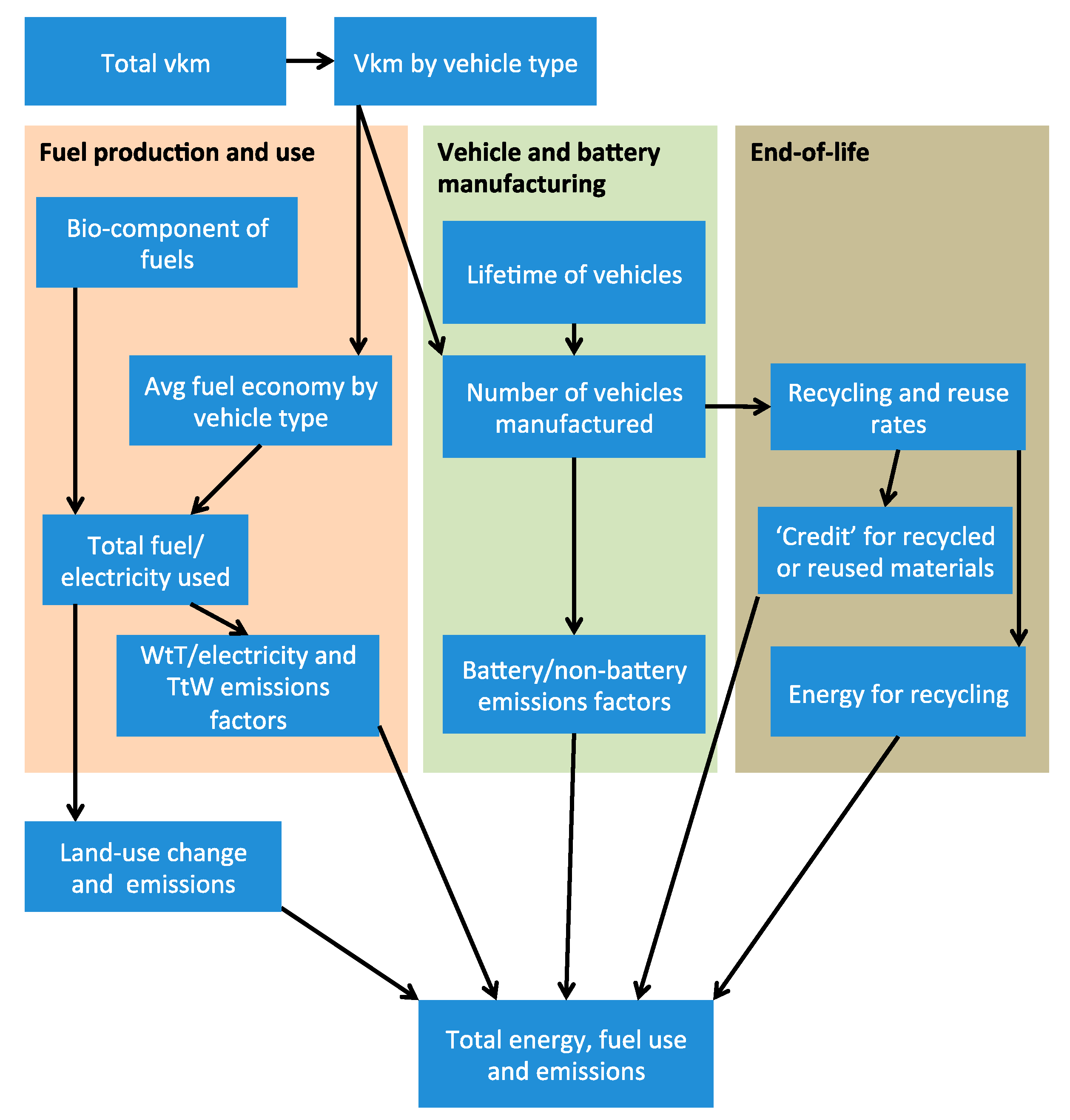
The LCA considers passenger cars, urban buses and bus rapid transit (BRT) buses. However, because the magnitude of results of BRT buses is negligible in comparison to the other modes (see Figure 4), the results for BRT are omitted for brevity. The LCA is calculated in a spreadsheet for the years 2015–2050 in five-year steps. The results for each year are for only the year in question as a ‘snapshot’ (i.e., the intervening years are ignored). An overview of the aspects and life phases considered in the LCA is shown in Figure 1, and further described in the section below. The spreadsheet is structured to allow for the comparison of sets of five scenarios, allowing a comparison of the BAU scenario with four alternatives. Appendix A contains tables of the input values used in the LCA.

2.1. Vehicle Use and Characteristics

2.1.1. Total National Vehicle Use

To allow free selection of various powertrain types (see below) in the scenarios, the total distance driven in Brazil by all vehicles of each mode (cars, urban buses) (Figure 2) per year in vehicle kilometers (vkm) must be calculated. It is calculated from the total projected vehicle stock of each mode multiplied by the corresponding average distance driven per vehicle, using figures for both from International Energy Agency (IEA) modeling [47,48] (

Table A4. Overall annual distance driven and fuel economy (liters of gasoline equivalent (LGe), per 100 km) for cars. Data from [47].

	2015	2020	2025	2030	2035	2040	2045	2050
Vehicle stock (million)	35.7	37.8	41.2	45.7	54.3	62,6	68.6	72.7
Average travel per vehicle	13,899	13,422	13,108	13,196	13,385	13,578	13,717	13,797
Total vkm (billion)	496.6	501.1	503.3	505.4	507.4	539.7	603.5	726.8
Fuel economy (LGe/100 km)
Diesel ICE	7.6	7.2	6.8	6.4	6.0	5.8	5.7	5.5
Diesel hybrid	6.1	4.8	4.9	4.9	4.9	4.9	4.8	4.8
Flex ICE	9.4	8.9	8.3	7.5	6.8	6.5	6.2	6.0
Flex hybrid	6.3	5.5	5.3	5.2	5.1	5.1	4.9	4.8
CNG/LPG	9.9	9.8	9.7	8.4	7.0	6.6	6.2	6.0
Electric	2.3	2.2	2.2	2.1	2.0	2.0	2.0	1.9

and

Table A5. Overall annual distance driven and fuel economy (liters of gasoline equivalent (LGe), per 100 km) for urban buses. Data from [47].

	2015	2020	2025	2030	2035	2040	2045	2050
Vehicle stock (thousand)	273.6	293.4	315.1	300.1	277.1	251.4	229.7	210.2
Average travel per vehicle	32,715	32,715	32,715	32,715	32,715	32,715	32,715	32,408
Total vkm (billion)	8.95	9.60	10.31	9.82	9.07	8.22	7.52	6.81
Fuel economy (LGe/100 km)
Diesel ICE	44.7	43.1	42.1	41.0	40.0	39.0	38.0	37.1
Diesel hybrid	34.7	33.6	32.7	31.9	31.1	30.3	29.6	28.8
Flex ICE	49.6	47.9	46.7	45.6	44.4	43.3	42.2	41.2
Flex hybrid	37.2	36.0	35.1	34.2	33.3	32.5	31.7	30.9
CNG/LPG	49.6	47.9	46.7	45.6	44.4	43.3	42.2	41.2
Electric	14.9	14.4	14.0	13.7	13.3	13.0	12.7	12.4

).

2.1.2. Fleet and Fuel Composition

In each scenario, for each year (

Table A2. Proportion of cars in the fleet by powertrain type for the various scenarios.

	2015	2020	2025	2030	2035	2040	2045	2050
BAU
Flex internal combustion engine (ICE)	0.95	0.96	0.98	0.97	0.95	0.92	0.88	0.82
Flex hybrid			0.01	0.03	0.05	0.07	0.11	0.16
Compressed natural gas (CNG)	0.05	0.04	0.01
BEV						0.01	0.01	0.02
Biofuel w/o hybrid
Flex ICE	0.95	1	1	1	1	1	1	1
Flex hybrid
CNG	0.05
BEV
Biofuel ½ hybrid
Flex ICE	0.95	0.9	0.84	0.77	0.7	0.63	0.56	0.5
Flex hybrid		0.1	0.16	0.23	0.3	0.37	0.44	0.5
CNG	0.05
BEV
Biofuel with hybrid
Flex ICE	0.95	0.81	0.68	0.54	0.4	0.26	0.12
Flex hybrid		0.19	0.32	0.46	0.6	0.74	0.88	1
CNG	0.05
BEV
Electrification
Flex ICE	0.95	0.82	0.67	0.54	0.4	0.27	0.14
Flex hybrid
CNG	0.05
BEV		0.18	0.33	0.46	0.6	0.73	0.86	1

and

Table A3. Proportion of urban buses in the fleet by powertrain type for the various scenarios.

	2015	2020	2025	2030	2035	2040	2045	2050
BAU
Diesel ICE	1	1	1	0.98	0.95	0.89	0.8	0.7
Diesel hybrid				0.01	0.03	0.06	0.1	0.15
CNG						0.01	0.01	0.01
BEV				0.01	0.02	0.04	0.09	0.14
Biofuel w/o hybrid
Diesel ICE	1	1	1	1	1	1	1	1
Diesel hybrid
CNG
BEV
Biofuel ½ hybrid
Diesel ICE	1	0.93	0.85	0.78	0.71	0.64	0.57	0.5
Diesel hybrid		0.07	0.15	0.22	0.29	0.36	0.43	0.5
CNG
BEV
Biofuel with hybrid
Diesel ICE	1	0.86	0.71	0.57	0.43	0.29	0.14
Diesel hybrid		0.14	0.29	0.43	0.57	0.71	0.86	1
CNG
BEV
Electrification
Diesel ICE	1	0.85	0.71	0.57	0.42	0.28	0.14
Diesel hybrid
CNG
BEV		0.15	0.29	0.43	0.58	0.72	0.86	1

), the composition of the fleets (cars and urban buses) is defined from the following powertrain types: flex, flex hybrid, diesel, diesel hybrid, compressed natural gas (CNG) and electric. Hybrids are assumed to be ‘standard’ hybrids without the facility to be charged from external sources, while electric is assumed to mean fully electric vehicles with only onboard batteries as energy storage. In parallel, for each year, the proportion of biofuels sold is defined from 0%–100% (

Table A1. Proportion of biofuels sold in Brazil in the various scenarios [49,50]. Fossil diesel and petrol make up the remaining portion.

	2015	2020	2025	2030	2035	2040	2045	2050
Proportion of biodiesel
BAU/electrification		0.100	0.100	0.100	0.100	0.100	0.100	0.100
Biofuel		0.143	0.286	0.429	0.571	0.714	0.857	1.000
Proportion of ethanol
BAU/electrification	0.496	0.560	0.560	0.560	0.560	0.560	0.560	0.560
Biofuel	0.496	0.568	0.640	0.712	0.784	0.856	0.928	1.000

). Values for the volume of fuels sold are available for 2015 and 2018 [49,50]; the 2020 values are calculated by extrapolating the development from 2015 to 2018. For ethanol, both hydrated and anhydrous are considered together; hence, the proportion in 2015 (49.6%) being significantly greater than the 27% ethanol as mandated in pump petrol (‘gasohol’). For biodiesel, the extrapolated 2020 value was above the mandated 10%; so, 10% has been used from 2020 onwards under the assumption that there would be no overshoot.

This model assumes all relevant vehicles are able to run on any proportion of bio or fossil fuel. For petrol, flex vehicles are near ubiquitous in new registrations in Brazil [41] (and ethanol is sold in similar volumes to petrol in 2015) and so this assumption is almost already reality. For diesel, however, Brazil’s pump diesel currently contains only 10% biodiesel, so this assumption must be considered more speculative, though it is assumed to be possible given sufficient research and development for the purposes of this LCA.

2.2. Fuel Production and Use Phase

2.2.1. Total Fuel Use Per Vehicle Type and Fuel Type

The total vkm per mode and powertrain type is calculated based on the overall vkm per mode and the powertrain proportions as entered in the scenarios. The total use-phase energy, and thus fuel, consumed by each vehicle type is calculated from the vkm and the corresponding on-road average fuel economy for each type. All relevant values here are provided by the IEA [47] (Table A4 and Table A5). The total amounts of fuel used are multiplied by emission factors for well-to-tank (WtT) (including electricity) and tank-to-wheel (TtW) emissions (more details of both below) to determine the emissions of each vehicle (and fuel) type and thus scenario. For electric vehicles, the round-trip efficiency for electric vehicles (buses) of 88%, from Lajunen [51], is applied to the stated fuel economy to reflect the inefficiency in charging and discharging the battery.

2.2.2. Well-to-Tank (WtT) Emissions

For each fuel type, the well-to-tank CO₂ emissions (per liter) are given by Edwards et al. [52] (

Table A7. Well to Tank (WtT) and Tank to Wheels (TtW) CO₂ emission factors for various fuels.

Fuel	Well to Tank (g/MJ)	Tank to Wheels (g/MJ)
Petrol	13.8	69.8
Ethanol	18.1	0.0
Diesel	15.4	74.4
Biodiesel	34.6	0.0
CNG	19.6	62.2

). The figures provided are calculated for Europe and modified for Brazil (see below), as consistent figures for all fuel types for Brazil could not be found. For fossil fuels, the figures have been used as found. For biofuels, the European figures for Brazilian-produced ethanol and biodiesel are modified by deducting the value listed for ‘transport to Europe’. These figures do not contain land-use emissions. The WtT factor for electric vehicles is provided by the relevant average emission intensity of the electricity system in that year (see below).

2.2.3. Tank-to-Wheels (TtW) Emissions

TtW emissions are calculated using the energy and CO₂ content of each fuel type [47,53], along with NOx and PM exhaust emissions intensities from Agência Nacional de Transportes Terrestres [54], supplemented with NOx exhaust emissions intensities for LPG/CNG vehicles from Murrells and Pang [55] (Table A7). The TtW CO₂ exhaust emission intensity of ethanol and biodiesel is considered to be zero as this carbon is considered to have been sequestered in the production phase. For NO_x and PM, the values for 2012 (the latest year available) are applied for all years (

Table A6. NO_x and PM emissions intensities (g/km) for 2012. [54].

Pollutant	Petrol	Ethanol	Diesel	CNG
NOx	0.0300	0.0300	2.1020	0.0310
PM	0.0011	0.0000	0.0200	0.0011

), or an annual reduction in air pollution emission intensity of 8.67% (from 2012), derived from Miller et al. [56] is applied.

2.2.4. Electricity System

Best- (mostly renewables) and worst-case (mostly fossil fuels) scenarios for both total generation (in TWh) and CO₂ emission intensity (in kilotonne/TWh) are provided by the online calculator provided by the Energy Research Office [57] (EPE in Portuguese) for decadal years (2020, 2030, etc.) (

Table A8. Total Brazilian electricity generation and CO₂ emissions intensities for 2015/17 [46] and EPE scenarios for the best and worst case [57] for 2020–2050.

Year	Generation (TWh)			CO2 Emissions Intensities (kiloton/TWh)
	2015/17	Best Case	Worst Case	2015/17	Best Case	Worst Case
2015	531 *	531 *	531 *	122 *	122 *	122 *
2020	547 **	857	837	94 **	88	147
2030	547 **	1197	1246	94 **	47	257
2040	547 **	1656	1743	94 **	37	317
2050	547 **	2260	2298	94 **	29	354

* Actual values from 2015; ** actual values from 2017.

), extrapolated to other years. The worst-case scenario is the default used in the scenarios. The model does not account for any effects of large additional loads in the short or long term, and the total generation capacity is used only as a comparison; a more complicated model accounting for the characteristics of the electricity generation system is beyond the scope of this study.

2.2.5. Land-Use Change Emissions

A direct land-use change (LUC) emission model is used to calculate the LUC emissions. It is assumed that the land area for all other crops remains the same, with all changes in biofuel use directly affecting the land used to grow the feedstocks, and that this land comes from (or returns to) various forest types or Cerrado/savannah according to the volume of biofuel needed in each year. A more complicated model involving intermediate steps and economic elasticities is beyond the scope of this analysis.

Firstly, the land area required to grow the requisite fuel feedstocks is calculated using figures for the yield of ethanol (sugarcane) or biodiesel (assumed to be all derived from soyabeans) per land area, using values from Valin et al. [58] (

Table A10. Biofuel yields [58] and applied values for LUC emissions of CO₂ for various biomes (from Table A9).

Aspect		Value
Biofuel yields per land area of cropland (L/ha)	Ethanol	5570
	Biodiesel	530
CO2 emissions from LUC (g/ha)	Cerrado (savannah)	121,845,050
	Plantation forest	211,755,493
	Low forest	283,641,324
	Avg forest	459,142,610
	High forest	634,643,895

). The values used are constant for all land types and locations. From this and the volume of fuel required each year, the yearly change in cropland area from the previous period is calculated.

The National Energy Policy Council (CNPE) has mandated, as part of the RenovaBio programme, a decrease in the CO₂ emissions of each unit of energy consumed by Brazilians from 74.3 g/MJ (2017) to 66.1 g/MJ in 2029; 1.07% per year [59], assumed to be achieved through increased biofuel yields (L/ha) and from increasing the proportion of biofuels used in fuels, though no statement of how much each contributes is given, and so it is assumed that each contributes half of the 1.07% (0.535% pa). The improved biofuel yields are thus increased at the rate of 0.535% per annum, although even this may be overly favorable to biofuels as the possibility of increased yields is questioned by Bernardo, Lourenzani, Satolo, and Caldas [60]. Furthermore, this would almost certainly cause the embedded CO₂ in biofuel to increase through, e.g., increased tractor and fertilizer use, and because these changes cannot be quantified, they are assumed to be negligible. The assumption that increased biofuel use decreases emissions presents a difficulty, as this is the opposite finding to this LCA, and so must be assumed to be based on a different methodology; as such, the other half of the mandated 1.07% decrease from increased biofuel use is omitted.

For biodiesel, 20% of the land-use change emissions are attributed to transport use, according to the ≈20% oil portion of the beans which can be used to make biodiesel: the other 80% would be attributed to the other uses of the soyabeans (e.g., soyameal for animal feed), outside this LCA.

Secondly, the carbon dioxide emitted (or absorbed) from the change in land-use is calculated using values of the carbon content of various Brazilian forest types (including plantation) and Cerrado (Brazilian Savannah) (

Table A9. Description of various methods and sources of carbon (not CO₂) content of Brazilian biomes.

Description	Value (Mg/ha)	Source
Author’s judgement of map of values for Amazon	360	[63]
Average of given values for Atlantic forest	230.8
Author’s judgement of map of values for Cerrado	60
“national-level forest AGB [above-ground biomass] density” with errors.	306.79 ± 36.1	[64]
“Estimates of forest carbon stocks” per canopy cover threshold (10%, 25% and 30%)	102, 116, 123	[65]
Plantation forest land area and AGB for 2016	104.3	[66]
Average forest AGB for four submodels (1990–2009 average)	199, 266, 200, 196	[61]

). The values for plantation forest and Cerrado are used as found, whereas a numerical mean and standard deviation is calculated for the forest values, with the low and high values representing one standard deviation from the mean value. The conversion from biomass carbon to CO₂ emissions is performed using the average ratio between “Average forest AGB [Above Ground Biomass]” and “Primary forest (instantaneous, non-process) emissions” (primary is selected assuming that the recropping of the land for biofuel is part of the secondary stage), from Aguiar et al. [61], giving a value for CO₂ emissions for each hectare of land changed.

The emissions from land-use change are spread over a 20 year period. LUC emissions in 2015 are zero as the LCA captures only change in biofuel use (and thus land use) to generate LUC emissions, and so for example the 2020 value includes any change from 2015 to 2020.

2.3. Vehicle and Battery Manufacturing Phase

For computational efficiency and because of a lack of equivalent model data pre-2015, a fleet model could not be implemented, so the number of vehicles manufactured per year is calculated by assuming each year is closed regarding vehicles, i.e., all vehicles used in a year would be manufactured in that year and disposed of at the end of the same year. The scenarios thus prescribe a fleet proportion, not sales proportions of the various powertrain types. The number of vehicles for each year is calculated by dividing the total vkm for each powertrain type by the total lifetime (in km) of that type. The emissions for vehicle manufacturing are constant per vehicle, independent of changes to the electricity emission intensity applied elsewhere in the LCA. In addition, the values are accounted for in Brazil, even if the parts actually originate elsewhere.

For cars, the lifetime (200,000 km) is provided by Messagie [14] and assumed to be the same for all vehicle types (see

Table A11. Vehicle and battery life and number of batteries required in cars’ lives.

Vehicle Type	Vehicle Life (km)	Battery Size (kWh)	Batteries in Vehicle Life	Battery Round Trip Efficiency
Flex ICE	200,000
Flex hybrid		1.5	1.5
CNG
BEV		30.0	1.5	0.88

). In addition, with the exception of the batteries for hybrid and electric vehicles, the non-battery components are assumed to result in the same CO₂ emissions (≈3.2 tonnes); see

Table A12. Total lifetime CO₂ emissions for cars (including fuel use) and the proportion of the total from manufacturing of the glider and powertrain (i.e., everything but the battery).

Component Proportions	Proportion	CO2 (g)
Total lifetime emissions (estimated, incl. fuel use)	−	17,680,000
Glider	0.15	2,652,000
Powertrain	0.03	530,400

. For buses, the lifetimes (different by powertrain type) are provided by Lajunen [51] with a correction factor for the lifetime of non-diesel buses in line with the calculations by WRI [62] (

Table A13. Vehicle and battery life and number of batteries required in urban bus lives.

Vehicle Type	Vehicle Life (km)	Battery Size (kWh)	Battery Life (km)	Batteries in Life	Battery Round Trip Efficiency
Diesel ICE	1,000,000
Diesel hybrid	1,200,000	14.5	190,000	6.3
Flex ICE	1,000,000
Flex hybrid	1,200,000	14.5	190,000	6.3
CNG/LPG	1,000,000
Electric	1,500,000	99.5	600,000	2.5	0.88

and

Table A14. Total manufacturing emissions for various bus types and their associated non-battery component where applicable.

Vehicle Type	Total	Total Non-Battery
Diesel ICE	45,400,000	45,400,000
Diesel hybrid	48,600,000	45,600,000
Flex ICE	45,400,000	45,400,000
Flex hybrid	48,600,000	45,600,000
CNG	45,400,000	45,400,000
Electric	56,900,000	40,800,000

).

Battery manufacturing emissions are calculated from the overall capacity of batteries required for all hybrid and electric vehicles and their respective battery capacities (and the rate of battery replacement) as shown in Table A11 and Table A13. A range of current battery manufacturing emissions intensities (in g/kWh) is provided in Hall and Lutsey [16], from which the average (default) minimum or maximum values (see

Table A15. CO₂ emissions intensities for battery manufacturing (in g/kWh).

Scenario	Manufacturing CO2 Emissions (g/kWh)
Minimum	30,000
Average	152,063
Maximum	494,000

) can be applied. The default assumption for the battery and vehicle manufacturing calculations is that both are manufactured from raw materials and disposed of without reuse or recycling at the end of life. As such, if the scenarios dictate that the materials (and thus CO₂ emissions) are recovered or reused at the end of life, this results in a ‘credit’, covered in more detail in the end-of-life section, below.

2.4. End-of-Life Phase

As mentioned above, the LCA treats each year as a closed system, so all vehicles used in any year also come to the end of their lives in that year. Five aspects of the end of life are considered: non-battery recycling emissions, non-battery materials credit, battery recycling emissions and materials credit and a battery reuse credit (values and sources given in

Table A16. End-of-life data and sources.

Aspect		Figure	Source
Energy for recycling	Vehicle	0.43 MJ/kg	[67]
	Battery	469 MJ/kWh
Mass (kg)	Car	1200	[40]
	Bus	7491	[51]
Extra emissions for all-virgin materials vehicle production		15–20%	[68]
Reduction in emissions by using recycled battery materials		23–43%	[69]
		10–17%	[68]
Current battery recycling rate		5%	[70]
Vehicle-use portion of battery life		58.1%	[69]

). Reusing batteries and recovering materials through recycling effectively reduces the manufacturing emissions, but they are considered as credits in this manner to allow separate (calculation) and presentation of these and the default manufacturing emissions.

Recycling emissions considers the energy required to recycle the respective parts and is calculated by multiplying the total mass of vehicles and capacity of batteries to be recycled by the respective factors for the energy required to recycle them. It is assumed the energy for this comes from the electricity network, so the relevant CO₂ emission intensity of the electricity system for that year is applied.

The vehicle recycling materials credit is included at current levels of recycling and use of recycled materials. The credit is zero as it is assumed to be included in current calculations of vehicle manufacturing emissions.

The battery recycling materials credit is calculated according to the 10%–17% and 23%–43% reductions (Table A16) given for the use of recycled materials in battery manufacturing. The base assumed reduction is 26.5%—the mid-point between the 10% and 43% outer figures. The actual emission credit figure is calculated from the total battery manufacturing emissions in the relevant year, multiplied by the 26.5% and the assumed proportion of battery recycling (details below).

The battery reuse credit is calculated using the assumed extra life (72%) batteries can be used for after their vehicular use, i.e., they are used for 58.1% of their lives in vehicles and, as such, the remaining 41.9% counted as a credit for this LCA, as that proportion of the manufacturing emissions can be attributed to subsequent use.

The calculation of end-of-life credits applies an assumed proportion of battery reuse and recycling. Both are assumed to increase linearly to 100% by 2050, from 5% and 0% in 2015 for recycling and reuse, respectively (see

Table A17. Battery recycling and reuse rates as applied in the LCAs.

Aspect	2015	2020	2025	2030	2035	2040	2045	2050
Battery recycling rate	0.05	0.19	0.32	0.46	0.59	0.73	0.86	1.00
Battery reuse rate		0.17	0.33	0.46	0.60	0.73	0.87	1.00

). This assumes that the greater use of batteries as per the scenarios will create an ever-greater economic and environmental imperative on the more efficient use of batteries and materials. As batteries can be both reused and recycled, both credits can be applied.

3. Scenarios Tested

Figure 3 shows the sets of scenarios examined (for each mode), consisting of a main LCA and four sensitivity analyses, considering LUC emissions, battery manufacturing emissions, vehicle and battery lives and electricity system developments vs. a best-case biofuel scenario, respectively. The content of the scenarios was defined based on a combination of the primary purpose of the study (comparing biofuels to electrification), the main factors affecting the results as described in the introduction and the intermediate results of the LCA itself. These are outlined in the following section, and the component parts are described in detail in Appendix A.

For all scenario values, where the user-input (i.e., non-modeled) values change between 2015 and 2050, the values for intervening years are changed linearly. All parameters for all scenarios in 2015 are set to the 2015 BAU values. All sub-LCAs contain the BAU as described in the main LCA.

3.1. Main LCA

An overview of the scenarios used for the LCA of cars is shown in

Table 2. Overview of the scenarios tested in the main LCA (values for 2015/20–2050, interpolated for intermediate years).

	BAU	Biofuel with Hybrid	Biofuel without Hybrid	Electrification, Best Case	Electrification, Worst Case
Fuels *	Ee50/56-Ee56	Ee50/57-Ee100		Ee50/56-Ee56
	B0/10-B10	B0/14-B100		B0/10-B10
Vehicles	Model	0%–100% hybrid	0%–0% hybrid	0%–100% electric
Electricity	Worst case			Best case	Worst case
Battery manuf.	Average
LUC	Average forest

* Analogous to the common naming convention whereby, e.g., E85 represents an 85%/15% ethanol/petrol mix as sold; ‘Ee’ (ethanol effective) represents the overall proportion of ethanol (hydrated and anhyrdous) to petrol, as if these were sold as a single mixed fuel, though in fact hydrated ethanol is sold from separate pumps by itself. B10 denotes 10% biodiesel, 90% fossil-diesel.

(details in Table A1, Table A2 and Table A3). The main LCA compares BAU to biofuel scenarios with and without hybridization, and electrification for the best- and worst-case electricity system development.

For the BAU scenario, the 2015/2020 proportions of ethanol (50% in 2015, 57% subsequently) and biodiesel (0% in 2015, 10% from 2020 onwards) are applied, while the vehicle proportions are provided from the IEA model [47].

The biofuel scenarios are based on the complete conversion of cars to ethanol and buses to biodiesel by 2050. As such, the proportions of biofuel in pump fuels are linearly increased to 100% in 2050 from the 2020 values: 57% for ethanol and 10% for biodiesel. In addition, the proportion of flex vehicles (for cars) or diesels (for buses) is linearly increased to 100% by 2050. Furthermore, the proportion of hybrid vehicles is increased to 100% in the biofuel and hybrid scenario but maintained at 0% in the biofuel without hybrid scenario. The few other vehicles are phased out by 2020.

Both electrification scenarios are based on the gradual shift toward complete electrification of cars and buses by 2050. The biofuel components of pump fuels as per BAU are used. The proportion of flex or diesel vehicles is linearly decreased to 0% by 2050, with hybrids contributing an ever-greater proportion of the total proportion allocated to flex or diesel vehicles. Other vehicle types (CNG, non-diesel buses) are phased out by 2020. Fully electric vehicles make up the remainder. The sole difference in the two electrification scenarios is the use of either the EPE best- or worst-case scenarios concerning total electricity generation and CO₂ emission intensity.

3.2. Sensitivity Analysis #1: Land-Use Change Emissions

This sensitivity analysis (

Table 3. Overview of the scenarios tested in the sensitivity analysis on LUC (values for 2015/20–2050, interpolated for intermediate years).

	BAU		Biofuel ½ Hybrid
	with LUC	without LUC	No LUC	Cerrado	Forest Density
					Plantation	Low	Avg	High
Fuels	Ee50/56-Ee56		Ee50/57-Ee100
	B0/10-B10		B0/14-B100
Vehicles	Model		0%–50% hybrid
Electricity	Worst case
Battery manuf.	Average
LUC	Avg forest	None	None	Cerrado	Plantation forest	Low forest *	Avg forest *	High forest *

* Refers to the carbon density of the forest per hectare.

) considers the effect of the biome used as the basis of land-use change (LUC) emissions on biofuel scenarios, i.e., the source of land used for extra land for biofuel feedstocks (or the inverse for diminishing demand). The scenarios are calculated (and presented) in two halves due to scenario-number limitations of the calculation tool.

The BAU scenario is used as per the main LCA, along with a BAU without LUC scenario, in which the LUC component is omitted. These are shown on both graphs for comparison.

Otherwise, six biofuel scenarios are calculated assuming the use of the biomes Cerrado, plantation forest, and low-, average- and high-density virgin forest, along with a scenario in which LUC emissions are omitted. These latter six LUC biome scenarios are applied to a biofuel scenario, splitting the difference between the ‘with’ and ‘without hybrid’ scenarios from the main LCA: the proportion of hybrids is increased linearly to 50% in 2050 (see Table A2 and Table A3).

3.3. Sensitivity Analysis #2: Battery Manufacturing Emissions

This sensitivity analysis (see

Table 4. Overview of the scenarios tested in the sensitivity analysis on battery manufacturing emissions (values for 2015/20–2050, interpolated for intermediate years).

	BAU	Biofuel, ½ Hybrid	Electrification
			Avg Battery Manuf.	Min Battery Manuf.	Max Battery Manuf.
Fuels	Ee50/56-Ee56	Ee50/57-Ee100	Ee50/56-Ee56
	B0/10-B10	B0/14-B100	B0/10-B10
Vehicles	Model	0%–50% hybrid	0%–100% electric
Electricity	Worst case
Battery manuf.	Average	Average	Average	Min	Max
LUC	Avg forest

) considers the effect on the electrification scenario of different values for battery manufacturing emissions. The values used are the average, minimum and maximum as presented in Hall and Lutsey [16]. These are applied to the (worst-case) electrification scenario from the main LCA and compared to the BAU and biofuel ½ hybrid scenarios from the main LCA and the sensitivity analysis, respectively.

3.4. Sensitivity Analysis #3: Vehicle and Battery Lives

This sensitivity analysis (see

Table 5. Overview of the scenarios tested in the sensitivity analysis on battery manufacturing emissions (values for 2015/20–2050, interpolated for intermediate years).

	BAU	Biofuel, ½ Hybrid	Electrification
			Default Lives	−20% Lives	+20% Lives
Fuels	Ee50/56-Ee56	Ee50/57-Ee100	Ee50/56-Ee56
	B0/10-B10	B0/14-B100	B0/10-B10
Vehicles	Model	0%–50% hybrid	0%–100% electric
Electricity	Worst case
Battery manuf.	Average	Average	Average	Min	Max
LUC	Avg forest
Vehicle and battery lives	Default		Default	Default −20%	Default +20%

) considers the effect on the electrification scenarios of changes to the effective life of both vehicles and batteries. Specifically, the lifetime of the vehicles and batteries (both expressed in km) is increased or decreased by 20%.

3.5. Sensitivity Analysis #4: Best-Case Biofuel Vs. Electricity System Development

This sensitivity analysis (see

Table 6. Overview of the scenarios tested in the sensitivity analysis on the best-case biofuel scenario vs. electrification under electricity system development scenarios (values for 2015/20–2050, interpolated for intermediate years).

	BAU	Biofuel with Hybrid	Electrification
			2015/17	Best Case	Worst Case
Fuels	Ee50/56-Ee56	Ee50/57-E100	Ee50/56-Ee56
	B0/10-B10	B0/14-B100	B0/10-B10
Vehicles	Model	0%–100% hybrid	0%–100% electric
Electricity	Worst case		2015/17	Best case	Worst case
Battery manuf.	Average
LUC	Avg forest	None	Avg forest

) compares a best-case biofuel scenario (full hybridization, no LUC emissions) with electrification scenarios under different electricity system developments regarding CO₂ emission intensity.

4. Results

The following contains an overview of the results of the various LCAs tested as described above. First, the main LCA results are shown, split into separate sections for cars and urban buses. This is followed by a section for the relevant results of each of the sensitivity analysis for both modes combined.

4.1. Main LCA

Figure 4 shows the CO₂ emissions of the BAU scenarios of cars, urban buses and BRT buses, respectively, in the main LCA. Cars are by far the dominant mode, while BRT buses are insignificant.

4.1.1. Cars

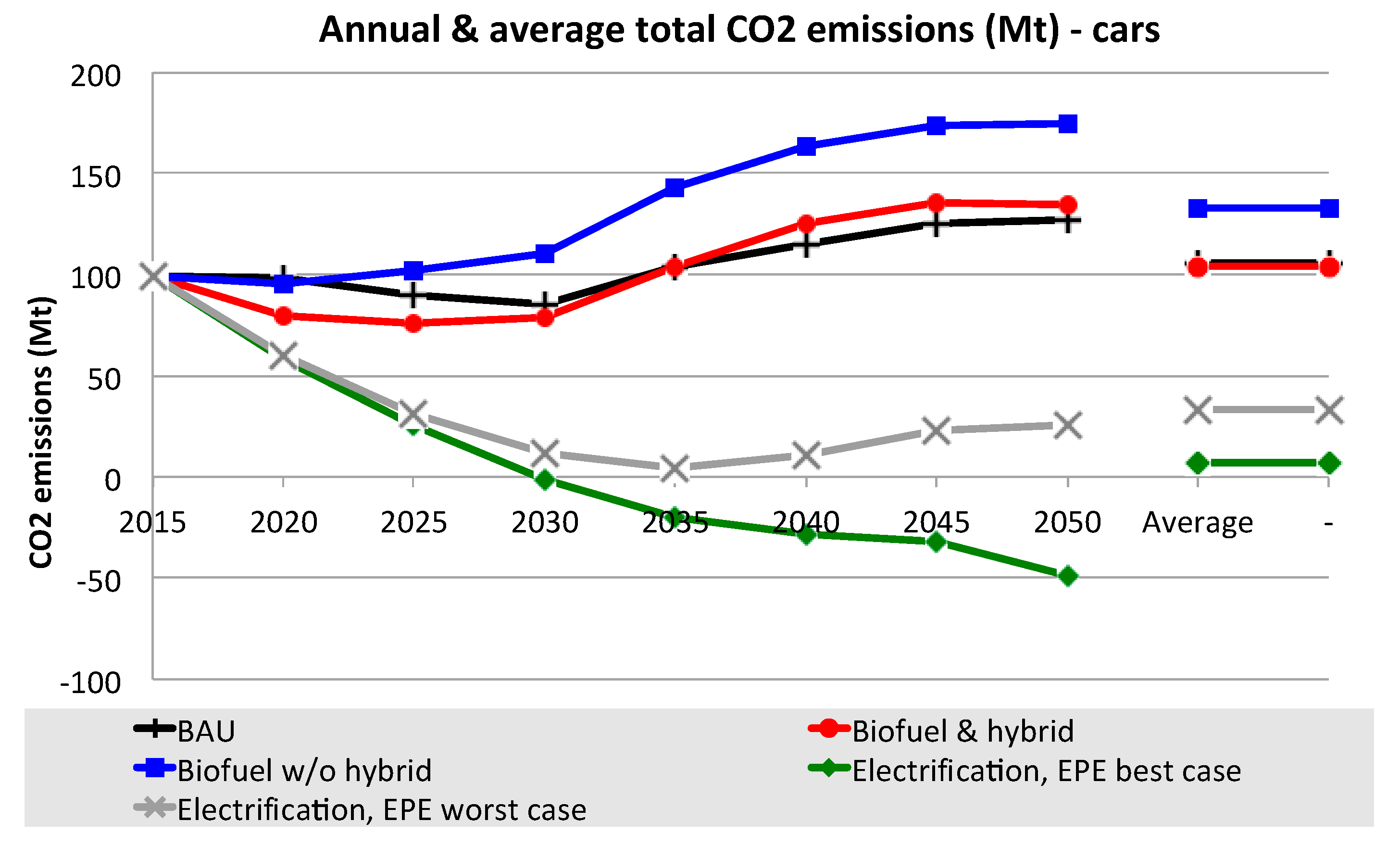
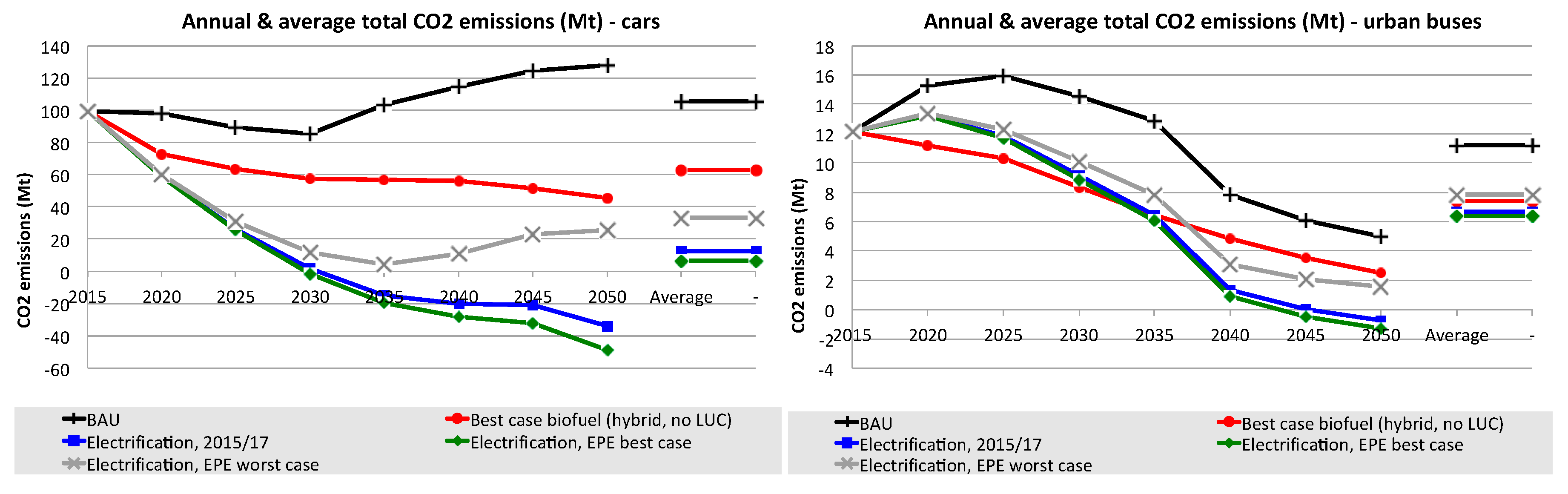
The results for the main LCA scenarios in Figure 5 show that the biofuel scenario without hybridization of the fleet has greater emissions than BAU on average, while biofuel with hybrid is approximately equal on average. Both electrification scenarios (best and worst case) have lower emissions than BAU throughout and on average.

Figure 6 shows the composition of the scenarios in the main LCA according to the different life phases in 2020, 2035 and 2050. The BAU scenario is predominated by exhaust emissions (grey), while the biofuel scenarios have large portions from LUC emissions (red), especially in 2035 and 2050. The electrification scenarios have large portions for manufacturing emissions (blue) in 2050, but in the best-case scenario, a great deal of those would be offset by the end-of-life credit for increased reuse and recycling of the parts and materials (black). In addition, this scenario is notable for the large negative portion of LUC emissions as the use of biofuel decreases and the land is switched to sequestration. In the worst-case electrification scenario, electricity generation (green) is a significant contributor to the overall emissions in 2050 due to the greater emission intensity of electricity generation in this scenario. For the same reason the end-of-life credit is diminished.

Figure 7 shows the result for air pollutant emissions in the main LCA scenarios. It shows electrification has a clear advantage over BAU. For NO_x, the biofuel scenarios have similar emissions to the (fossil-dominated) BAU scenario, while the air pollutant emissions for the electrification scenarios reduce to zero. For PM emissions, all alternatives to BAU have lower emissions. However, as shown in Figure 8, if policies and technologies are applied which contribute to an 8.67% annual improvement, as suggested by Miller et al. [56], the differences in powertrain technology become much less pronounced and all scenarios reduce to much lower levels by 2050.

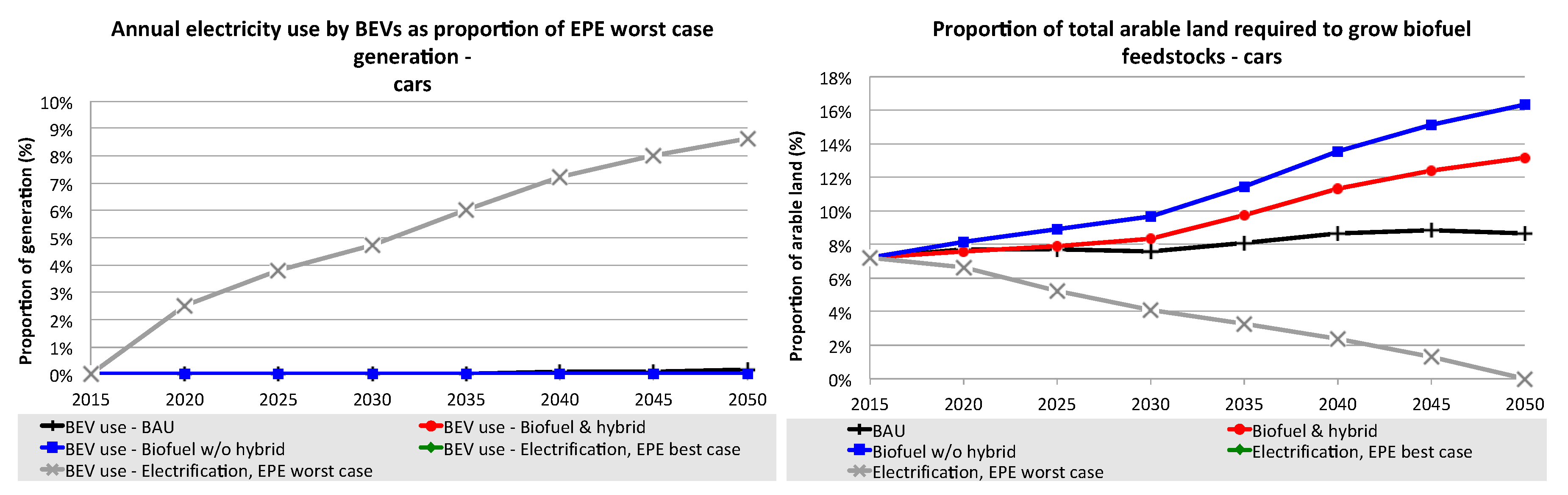
Figure 9 shows the results of the electricity consumption (left) and land use (right). The amount of electricity consumed steadily increases, approaching 9% of the worst-case generation capacity. The proportion of the arable land area required to meet the demand for ethanol increases steadily to over 13% and 16% in 2050 for the hybrid and non-hybrid scenarios, respectively.

4.1.2. Urban Buses

The results of the main LCA for urban buses (Figure 10) follow a similar pattern (between scenarios) as for cars, above. The electrification of urban buses would result in the lowest CO₂ emissions, with the two biofuel scenarios resulting in the greatest emissions. However, on a yearly basis, the hybrid biofuel scenario becomes lower than BAU by 2050, as the overall use of fuel reduces and much of the land previously used to grow biofuel feedstocks switches to sequestration. The biofuel scenarios are sensitive to the gradient of vehicle use. This holds for cars also, but there are several differences which account for the greater variation for urban buses.

• Urban bus use increases in the early stages of the analysis, where car use does not.
• Biodiesel results in greater LUC emissions per liter because of the lower yield per hectare of land.
• The scenarios dictate a greater increase per slot for biodiesel, which starts at zero and increases to 100% (≈14% per 5-year slot), whereas ethanol starts from ≈50%.

The composition of the total emissions according to life phases for urban buses (Figure 11) is also similar in pattern to cars. The biofuel scenarios have large land-use change emissions, especially in 2035, and the worst-case electrification scenario has large electricity generation emissions. Manufacturing and end-of-life emissions make only very small or insignificant contributions. This figure also shows the source of the negative overall emissions calculated for the best-case electrification scenario: primarily, the large negative emissions from LUC, as biofuel use is reduced.

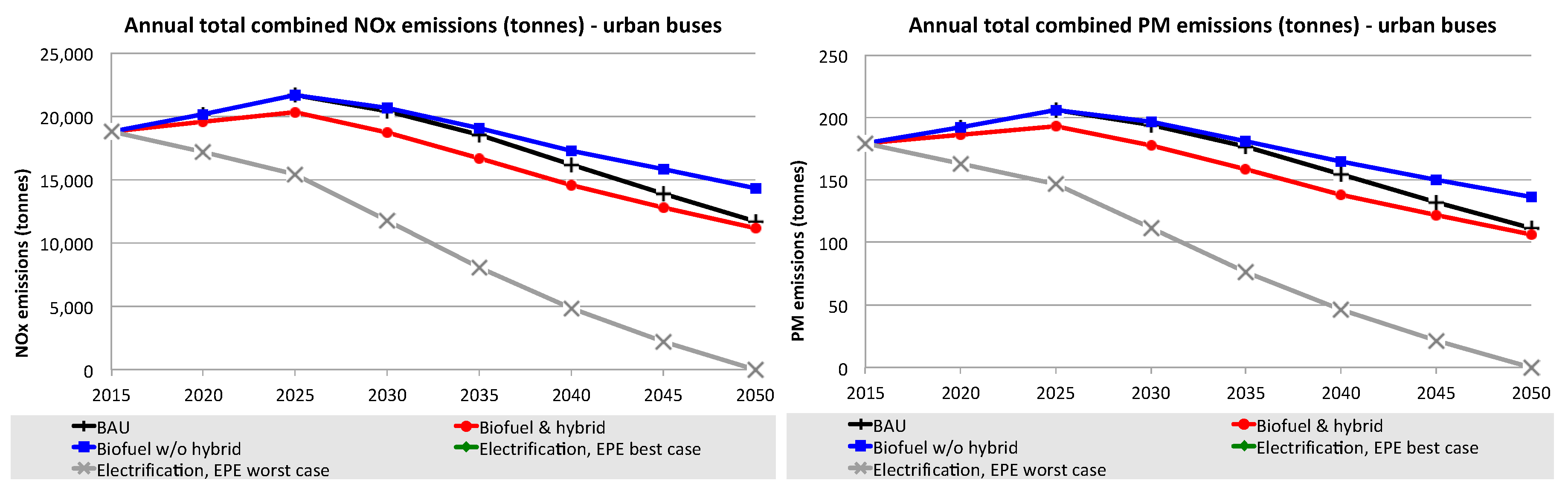
Also regarding air pollutant emissions, the same pattern emerges as for cars, as shown in Figure 12. The results and expected trends are similar to those of the car scenarios, with the biofuel scenarios without and with hybrid close to, but above and below, BAU, respectively, while the electrification scenarios steadily decrease to zero. However, as shown in Figure 13, if policies and technologies are applied which contribute to a 8.67% annual improvement, as suggested by Miller et al. [56], the differences in powertrain technology become much less pronounced and the emissions from all scenarios diminish to much lower levels by 2050.

Figure 14 shows the results of proportional electricity consumption (left) and proportional land use (right). Regarding electricity use, electric urban bus electricity consumption peaks at below 0.5%, presumably an irrelevant amount from a grid-operational perspective. The amount of land required to grow sufficient biofuel feedstocks for urban buses peaks at below 1% for the highest scenario: biofuels without hybrid, while the biofuel with hybrid scenario peaks at below 0.8%.

4.2. Sensitivity Analysis #1: Land-Use Change Emissions (Biofuel)

The total annual CO₂ emissions for the sensitivity analysis of various LUC emission scenarios are shown in Figure 15, below. Also included, for perspective, are the results for BAU if the LUC emissions were disregarded.

For both cars and urban buses, the results are quite sensitive to the LUC scenario selected, with a considerable difference between the biofuel scenarios with no-LUC (blue, left) and high-density forest (grey, right), in line with the overall contribution of LUC emissions to the overall result and the CO₂ embedded in the various biomes (values in t/ha), Cerrado (122, green, left), plantation forest (212, grey, left), then low- (284, blue, right), average- (459, green, right) and high-density forest (635, grey, right).

For cars, on average, the plantation forest, Cerrado and low-density forest biomes result in lower overall emissions than BAU; the average- and high-density forest biomes result in greater overall emissions than BAU.

For buses, if the land for biofuel feedstocks is assumed to come from/return to Cerrado or plantation forest, on average, the results are lower than BAU, with all remaining forest biomes resulting in greater emissions than BAU.

Furthermore, the difference between BAU with (black) and without (red) LUC emissions can be seen; for cars, BAU without LUC is consistently below BAU, but for urban buses, the same holds until between 2035 and 2040, where the lines cross due to the LUC emissions switching to sequestration in the BAU scenario.

In addition, in general, it can be seen that the results are also quite sensitive to year-to-year changes of fuel use.

4.3. Sensitivity Analysis #2: Battery Manufacturing Emissions

This sensitivity analysis examines the effect of battery manufacturing emissions on a CO₂ per kWh of battery capacity basis. The results are shown in Figure 16, showing that the overall results are not particularly sensitive to this change for cars, and practically not at all for urban buses.

4.4. Sensitivity Analysis #3: Vehicle and Battery Lives

This sensitivity analysis examines the effect of a this change in the life-length (both expressed in km) of both vehicles and their batteries in the electrification scenarios. For example, in the −20% scenario, the life of a car is reduced from 200,000 km to 160,000 km, in conjunction with a decrease in battery life from ≈133,000 km to ≈107,000 km. This has the effect of needing a greater (or lower) number of vehicles and batteries to be manufactured each year, with a corresponding change in the overall proportion of manufacturing emissions. Figure 17 shows the results for CO₂ emissions with a ±20% change in the assumed vehicle and battery life. For cars, this has a comparatively small effect, especially when compared to the difference to the BAU and biofuel scenarios shown. For urban buses, the effect is even smaller; it is practically invisible.

The final sensitivity analysis compares a best-case biofuel scenario with the three electrification scenarios, the results of which are shown in Figure 18. As this shows, all alternative scenarios have lower emissions than BAU, throughout and on average. Furthermore, on average, for cars the worst-case electrification scenario results in lower emissions than the best-case biofuel scenario, though the two do converge somewhat by 2050. For urban buses, all electrification scenarios initially rise above the best-case biofuel scenario but subsequently drop below.

4.5. Sensitivity Analysis #4: Best-Case Biofuel vs. Electricity System Development

Overall, this sensitivity analysis shows the advantage of the electrification scenarios over biofuels: even in what could be regarded as extreme and unrealistic scenarios, (biofuel disregarding LUC emissions altogether, and electrification dominated by fossil fuels), for cars, electrification still has lower emissions on average and throughout, and for urban buses, on average the result is only slightly in favor of the biofuel scenario. As such, under more realistic scenarios, it could be expected that electrification would have lower emissions.

Finally, the results presented here show that if the current overall CO₂ emission intensity of Brazilian electricity generation is maintained into the future (i.e., as per the 2015/17 scenario), the resulting emissions would be between the EPE scenarios, but closer to the best case, i.e., the worst-case scenario is significantly more CO₂ emission-intensive than the current scenario, and the best-case scenario is somewhat less CO₂ emission-intensive.

5. Findings and Discussion

1. Cars are the largest contributor to the effects examined in this LCA

Overall, of the modes examined in this LCA, cars have the greatest effect on the results—CO₂ emissions, air pollutant emissions, electricity consumption and land-use for biofuel feedstocks—albeit to differing degrees: the results for air pollutant emissions, for example, between cars and urban buses are comparatively close. Despite cars being smaller and having lower emissions per distance driven than buses, their collective total distance driven is much, much higher, accounting for their greater overall effect.

2. Electrification results in the lowest CO₂ emissions

This LCA finds that the lowest CO₂ emissions would be reached in the electrification scenarios examined. Even if the worst-case electrification scenario is compared to the best-case biofuel scenario—both of which are probably unlikely given the extremity of their underlying premises—the electrification scenario results in lower (cars) or only slightly higher (urban buses) emissions. In the main LCA, the electrification scenarios offer 65%–89% CO₂ savings over BAU on average (note that the electrification scenarios include negative LUC emissions). A comparison of this finding with the other electrification-biofuel comparison found [34] is near-impossible due to the very different methodologies applied (including an apparent exclusion of LUC emissions) and the different countries in question.

Not shown above is a further expansion of sensitivity analysis #4, in which the electrification scenarios were calculated without LUC emissions. For cars, the average CO₂ emissions were almost identical between the biofuel (with hybrid) and electrification (2015/17) scenarios. For urban buses, the biofuel scenario resulted in near-identical CO₂ emissions to the worst-case electrification scenario, i.e., without LUC at all, the BEVs offer improved CO₂ emissions, assuming the overall generation profile remains similar to the present. While there is controversy regarding the methodology of including LUC emissions, we consider it unlikely that LUC would be zero; however, even if it were, BEVs under reasonable assumptions would result in similar CO₂ emissions to biofuel with full hybridization.

3. Electrification results in lower air pollutant emissions

As with the CO₂ emissions, the results suggest that the electrification of cars and buses would be the ideal path as it would lead to the highest reduction in both NO_x and PM emissions. Biofuels, on the other hand, in most cases, do not reduce air pollution significantly from BAU (except for car PM emissions from ethanol). The magnitude of this result is greatly diminished; however, if a yearly improvement of ≈9% in emission intensity is achieved, the difference between scenarios becomes much smaller.

4. Land-use change emissions are a major contributor to the results for the biofuel scenarios

LUC emissions as calculated here are a major contributor to the overall CO₂ emissions of the biofuel scenarios, and there is a great difference between the carbon content of the biomes selected, making the results very sensitive to whether LUC emissions are included or how they are calculated, and the rate of change of vehicle/biofuel use. If the Cerrado or plantation forest biomes are used to calculate LUC emissions, the result is emissions below BAU level, while using average- or high-density forest results in higher-than-BAU emissions, with low-density forest being below BAU for cars, above for urban buses.

LUC emissions are delayed and for a limited time (20 years), but the other emissions occur on a year-by-year basis. An interesting aspect of this analysis, covering a long timeframe, is that it shows the way in which LUC emissions fluctuate in relation to the other emissions that occur on a year-to-year basis, which LCAs of a single point in time would be unable to show well.

Related to this point is the land that would be required to grow sufficient feedstocks for biofuels. For cars, assuming the worst case of the full use of biofuels (without hybridization), up to 16% of Brazil’s arable land would be required to grow sufficient sugarcane.

5. Electrification is sensitive to electricity system characteristics

While the electrification scenarios can potentially yield significant benefits in terms of emission reduction, the amount of benefit depends greatly on the electricity system’s average emission intensity. However, the analysis suggests capacity can be added with higher than current emission intensity (as per the EPE worst case) while still maintaining a significant benefit over BAU. This is in line with the findings of previous studies described in the introduction.

Another characteristic of the electricity system of note is the total generation capacity. This analysis shows that cars would result in significant electricity demand: the full-scale electrification of cars is calculated to require up to ≈9% (in 2050) of the projected total generation capacity of Brazil (38% of 2017-level generation capacity). Intuitively, this would also be significant in terms of peak loads. The electrification of urban buses is calculated to result in urban bus electricity demand that would remain below 0.6% of the total expected national generation capacity.

Other aspects

Similar patterns were found for the sensitivity of the results to battery manufacturing emission factors and the lifetime of vehicles and batteries. Namely, for cars, the overall result was not particularly sensitive to changes, while for urban buses, the overall result was hardly sensitive at all. Presumably, this is due to the relatively lower proportion of the manufacturing phase for urban buses. This is particularly interesting because it is in contrast to many sources in the introduction, suggesting both of these factors are strong determinants of the overall result.

The other effects listed in the literature review: charging time of day, noise, and other effects were beyond the scope of this study.

5.1. Policy Recommendations

Cars

From a CO₂ and air pollutant emissions standpoint, ideally, Brazil should implement policies to encourage the increased adoption of electric cars. These could include taxation or feebate schemes based on exhaust CO₂ emissions, subsidies on the purchase of electric vehicles, or free parking or use of carpooling lanes. As included in Rota 2030, manufacturers could be forced to include and encourage EVs by setting average emission levels targets (which decrease year by year) for all vehicles they sell each year, such as applies in the EU. Subsidies on locally manufactured fuels (including biofuels) should be removed or reduced

If electrification is not pursued, the use of ethanol should not be increased, by (at least) maintaining the current ≈50% proportion of ethanol (to petrol) sold.

Urban buses

The recommended course of action for urban buses is, superficially, the same as for cars: from a CO₂ and air pollution emissions standpoint, urban buses should be electrified. Electrification of urban buses may be easier than cars because biodiesel is not as well established or widespread in Brazil, and there are far fewer vehicles, and those vehicles tend to be owned and operated by organizations with many vehicles each, limiting the number of affected stakeholders. Given the far lower consumption of urban buses combined, less regard needs to be paid to considerations of the grid or overall generation capacity; though given that buses may need (very) high power, some local improvements may be necessary. Electrification of urban buses could be encouraged by providing direct funding to operators or local authorities to buy electric buses or the necessary charging infrastructure. Furthermore, where routes are put to tender, these could have the condition of being operated by electric vehicles.

General

Several aspects not covered directly by this LCA are nevertheless important regarding the discussion on reducing the emissions from the transport sector. These include measures to reduce the per km fuel consumption (and air pollution emissions) of individual vehicles, reducing the use of vehicles through improved urban planning and improved cycling and walking infrastructure and encouraging public transport use rather than individual vehicles, which would have positive effects on all aspects considered in this LCA, as well as in other dimensions not covered (e.g., health, noise, economics, etc.).

Another aspect to consider is the international aspect of technological development. Brazil’s biofuel system is very well developed, with arguably significantly better environmental outcomes than other countries, especially those using corn-ethanol. If all other countries shift away from liquid-fueled, internal-combustion vehicles to electric vehicles, this could make Brazil a technology island; potentially cut off from foreign sources of major developments such as autonomous vehicles, forcing Brazil to either develop those technologies themselves or adapt them to local vehicles.

Moreover, it is important to bear in mind the economic relevance of the biofuel industry in Brazil and its linkages to other sectors such as automotive. As such, if an electrification strategy for the automotive sector were implemented, consideration should be paid to the associated conversion of the biofuel industry.

Biofuel feedstocks and land

In all cases, but especially where the policy focus remains on biofuels, it should be ensured that any additional land used to grow biofuel feedstocks should not have high stored carbon, i.e., should be Cerrado or plantation forest, or similar biomes, or even better that it must come from already cleared land, such as farmland used for other crops, degraded pastureland or brownfield sites. However, steps must be taken to ensure any resulting pressure on farmland does not result in land cleared for other crops, and thus indirect land-use change emissions and productive ecosystems and the services they offer are not degraded.

As included in the yearly increase in biofuel feedstock yields, efforts to increase the yield of biofuels per area of land should be undertaken, such as investing in technological and capacity building. It must be noted though that this study does not include the assessment of impacts on other parameters such as soil biodiversity and sustainability, which might be important to consider if higher yield intensities are sought for existing areas of feedstock cultivation.

Electricity system

If electrification is pursued, especially for cars, the country’s electricity generation capacity should be increased in line with the consumption of BEVs. This added capacity should be as low emission as possible. Additionally, policies to address the possible high load on the grid of vehicles being charged should be implemented. At their simplest, these could involve simple grid/generation capacity upgrades. Preferential tariffs for off-peak charging could be introduced, possibly also in conjunction with technologies to allow vehicles to take advantage of those tariffs and also potentially for them to be utilized for grid balancing. Furthermore, the availability of charging infrastructure away from home would encourage people to buy EVs in the first place by easing their range anxiety, but also to charge their cars during the day away from the morning and evening peaks.

5.2. Suggested Improvements to the LCA Methodology Applied

The following areas have been identified as areas that would improve the LCA.

• A more complicated LUC calculation including the agricultural land-use elasticities and yields of biofuels differentiated by land type.
• Inclusion of modal/behavioral shift aspects to allow the effects of reduced travel or modal shifts to be included in scenarios.
• Inclusion of electricity emissions intensities in all aspects of the LCA (e.g., manufacturing) to better reflect changes to the system, along with better representation of the place of manufacture (and CO₂ emissions) of vehicle components.
• Consideration of the economic effects of hybrids and BEVs in Brazil, and of the expansion in electricity generation necessary for the electrification scenarios.
• Include a fleet model for vehicles.
• Inclusion of further effects such as water use (especially for biofuel feedstock production), toxicity, and the use of other key materials

References

- Hawkins, T.R.; Singh, B.; Majeau-Bettez, G.; Strømman, A.H. Comparative Environmental Life Cycle Assessment of Conventional and Electric Vehicles. J. Ind. Ecol. 2013, 17, 53–64. [Google Scholar] [CrossRef]
- Garcia, R.; Gregory, J.; Freire, F. Dynamic fleet-based life-cycle greenhouse gas assessment of the introduction of electric vehicles in the Portuguese light-duty fleet. Int. J. Life Cycle Assess. 2015, 20, 1287–1299. [Google Scholar] [CrossRef]
- Abdul-Manan, A.F.N. Uncertainty and differences in GHG emissions between electric and conventional gasoline vehicles with implications for transport policy making. Energy Policy 2015, 87, 1–7. [Google Scholar] [CrossRef]
- Ma, H.; Balthasar, F.; Tait, N.; Riera-Palou, X.; Harrison, A. A new comparison between the life cycle greenhouse gas emissions of battery electric vehicles and internal combustion vehicles. Energy Policy 2012, 44, 160–173. [Google Scholar] [CrossRef]
- Aguirre, K.; Eisenhardt, L.; Lim, C.; Nelson, B.; Norring, A.; Slowik, P.; Tu, N.; Rajagopal, D.D. Lifecycle Analysis Comparison of a Battery Electric Vehicle and a Conventional Gasoline Vehicle; UCLA IoES: Los Angeles, CA, USA, 2012. [Google Scholar]
- Van Mierlo, J.; Messagie, M.; Rangaraju, S. Comparative environmental assessment of alternative fueled vehicles using a life cycle assessment. Transp. Res. Procedia 2017, 25, 3435–3445. [Google Scholar] [CrossRef]
- Notter, D.A.; Gauch, M.; Widmer, R.; Wäger, P.; Stamp, A.; Zah, R.; Althaus, H.-J. Contribution of Li-Ion Batteries to the Environmental Impact of Electric Vehicles. Environ. Sci. Technol. 2010, 44, 6550–6556. [Google Scholar] [CrossRef] [PubMed]
- Hawkins, T.R.; Gausen, O.M.; Strømman, A.H. Environmental impacts of hybrid and electric vehicles—A review. Int. J. Life Cycle Assess. 2012, 17, 997–1014. [Google Scholar] [CrossRef]
- Tagliaferri, C.; Evangelisti, S.; Acconcia, F.; Domenech, T.; Ekins, P.; Barletta, D.; Lettieri, P. Life cycle assessment of future electric and hybrid vehicles: A cradle-to-grave systems engineering approach. Chem. Eng. Res. Des. 2016, 112, 298–309. [Google Scholar] [CrossRef]
- Peters, J.F.; Baumann, M.; Zimmermann, B.; Braun, J.; Weil, M. The environmental impact of Li-Ion batteries and the role of key parameters—A review. Renew. Sustain. Energy Rev. 2017, 67, 491–506. [Google Scholar] [CrossRef]
- Zackrisson, M.; Avellán, L.; Orlenius, J. Life cycle assessment of lithium-ion batteries for plug-in hybrid electric vehicles–Critical issues. J. Clean. Prod. 2010, 18, 1519–1529. [Google Scholar] [CrossRef]
- Majeau-Bettez, G.; Hawkins, T.R.; Strømman, A.H. Life Cycle Environmental Assessment of Lithium-Ion and Nickel Metal Hydride Batteries for Plug-In Hybrid and Battery Electric Vehicles. Environ. Sci. Technol. 2011, 45, 4548–4554. [Google Scholar] [CrossRef] [PubMed]
- Ellingsen, L.A.-W.; Hung, C.R.; Strømman, A.H. Identifying key assumptions and differences in life cycle assessment studies of lithium-ion traction batteries with focus on greenhouse gas emissions. Transp. Res. Part Transp. Environ. 2017, 55, 82–90. [Google Scholar] [CrossRef]
- Messagie, M. Life Cycle Analysis of the Climate Impact of Electric Vehicles; Transport & Environment: Brussels, Belgium, 2017. [Google Scholar]
- Ambrose, H.; Kendall, A. Effects of battery chemistry and performance on the life cycle greenhouse gas intensity of electric mobility. Transp. Res. Part Transp. Environ. 2016, 47, 182–194. [Google Scholar] [CrossRef]
- Hall, D.; Lutsey, N. Effects of Battery Manufacturing on Electric Vehicle Life-Cycle Greenhouse Gas Emissions; International Council on Clean Transportation: Washington, DC, USA, 2018; p. 12. [Google Scholar]
- Peters, J.F.; Weil, M. Providing a common base for life cycle assessments of Li-Ion batteries. J. Clean. Prod. 2018, 171, 704–713. [Google Scholar] [CrossRef]
- Bauer, C.; Hofer, J.; Althaus, H.-J.; Del Duce, A.; Simons, A. The environmental performance of current and future passenger vehicles: Life cycle assessment based on a novel scenario analysis framework. Appl. Energy 2015, 157, 871–883. [Google Scholar] [CrossRef]
- Woo, J.; Choi, H.; Ahn, J. Well-to-wheel analysis of greenhouse gas emissions for electric vehicles based on electricity generation mix: A global perspective. Transp. Res. Part Transp. Environ. 2017, 51, 340–350. [Google Scholar] [CrossRef]
- Wu, Y.; Zhang, L. Can the development of electric vehicles reduce the emission of air pollutants and greenhouse gases in developing countries? Transp. Res. Part Transp. Environ. 2017, 51, 129–145. [Google Scholar] [CrossRef]
- Onat, N.C.; Kucukvar, M.; Tatari, O. Conventional, hybrid, plug-in hybrid or electric vehicles? State-based comparative carbon and energy footprint analysis in the United States. Appl. Energy 2015, 150, 36–49. [Google Scholar] [CrossRef]
- Varga, B.O. Electric vehicles, primary energy sources and CO2 emissions: Romanian case study. Energy 2013, 49, 61–70. [Google Scholar] [CrossRef]
- Onn, C.C.; Chai, C.; Abd Rashid, A.F.; Karim, M.R.; Yusoff, S. Vehicle electrification in a developing country: Status and issue, from a well-to-wheel perspective. Transp. Res. Part Transp. Environ. 2017, 50, 192–201. [Google Scholar] [CrossRef]
- Hofmann, J.; Guan, D.; Chalvatzis, K.; Huo, H. Assessment of electrical vehicles as a successful driver for reducing CO2 emissions in China. Appl. Energy 2016, 184, 995–1003. [Google Scholar] [CrossRef]
- Zhou, G.; Ou, X.; Zhang, X. Development of electric vehicles use in China: A study from the perspective of life-cycle energy consumption and greenhouse gas emissions. Energy Policy 2013, 59, 875–884. [Google Scholar] [CrossRef]
- Ke, W.; Zhang, S.; He, X.; Wu, Y.; Hao, J. Well-to-wheels energy consumption and emissions of electric vehicles: Mid-term implications from real-world features and air pollution control progress. Appl. Energy 2017, 188, 367–377. [Google Scholar] [CrossRef]
- Shi, X.; Wang, X.; Yang, J.; Sun, Z. Electric vehicle transformation in Beijing and the comparative eco-environmental impacts: A case study of electric and gasoline powered taxis. J. Clean. Prod. 2016, 137, 449–460. [Google Scholar] [CrossRef]
- Jochem, P.; Doll, C.; Fichtner, W. External costs of electric vehicles. Transp. Res. Part Transp. Environ. 2016, 42, 60–76. [Google Scholar] [CrossRef]
- Faria, R.; Marques, P.; Moura, P.; Freire, F.; Delgado, J.; de Almeida, A.T. Impact of the electricity mix and use profile in the life-cycle assessment of electric vehicles. Renew. Sustain. Energy Rev. 2013, 24, 271–287. [Google Scholar] [CrossRef]
- Rangaraju, S.; De Vroey, L.; Messagie, M.; Mertens, J.; Van Mierlo, J. Impacts of electricity mix, charging profile, and driving behavior on the emissions performance of battery electric vehicles: A Belgian case study. Appl. Energy 2015, 148, 496–505. [Google Scholar] [CrossRef]
- Huo, H.; Cai, H.; Zhang, Q.; Liu, F.; He, K. Life-cycle assessment of greenhouse gas and air emissions of electric vehicles: A comparison between China and the U.S. Atmos. Environ. 2015, 108, 107–116. [Google Scholar] [CrossRef]
- Garcia, R.; Freire, F. A review of fleet-based life-cycle approaches focusing on energy and environmental impacts of vehicles. Renew. Sustain. Energy Rev. 2017, 79, 935–945. [Google Scholar] [CrossRef]
- Choma, E.F.; Ugaya, C.M.L. Environmental impact assessment of increasing electric vehicles in the Brazilian fleet. J. Clean. Prod. 2017, 152, 497–507. [Google Scholar] [CrossRef]
- Meier, P.J.; Cronin, K.R.; Frost, E.A.; Runge, T.M.; Dale, B.E.; Reinemann, D.J.; Detlor, J. Potential for Electrified Vehicles to Contribute to U.S. Petroleum and Climate Goals and Implications for Advanced Biofuels. Environ. Sci. Technol. 2015, 49, 8277–8286. [Google Scholar] [CrossRef] [PubMed]
- Finkbeiner, M. Indirect Land Use Change–Science or Mission? BioResources 2014, 9, 3755–3756. [Google Scholar] [CrossRef]
- Searchinger, T.; Heimlich, R.; Houghton, R.A.; Dong, F.; Elobeid, A.; Fabiosa, J.; Tokgoz, S.; Hayes, D.; Yu, T.-H. Use of U.S. Croplands for Biofuels Increases Greenhouse Gases Through Emissions from Land-Use Change. Science 2008, 319, 1238–1240. [Google Scholar] [CrossRef] [PubMed]
- Lapola, D.M.; Schaldach, R.; Alcamo, J.; Bondeau, A.; Koch, J.; Koelking, C.; Priess, J.A. Indirect land-use changes can overcome carbon savings from biofuels in Brazil. Proc. Natl. Acad. Sci. USA 2010, 107, 3388–3393. [Google Scholar] [CrossRef] [PubMed] [Green Version]
- Sanchez, S.T.; Woods, J.; Akhurst, M.; Brander, M.; O’Hare, M.; Dawson, T.P.; Edwards, R.; Liska, A.J.; Malpas, R. Accounting for indirect land-use change in the life cycle assessment of biofuel supply chains. J. R. Soc. Interface 2012, 9, 1105–1119. [Google Scholar] [CrossRef] [PubMed]
- Dunn, J.B.; Han, J.; Seabra, J.; Wang, M. Biofuel Life-Cycle Analysis. In Handbook of Bioenergy Economics Policy: Volume II; Springer: New York, NY, USA, 2017; pp. 121–161. [Google Scholar]
- Dallmann, T.; Façanha, C. International Comparison of Brazilian Regulatory Standards for Light-Duty Vehicle Emissions. In White Paper; International Council on Clean Transportation (ICCT): Washington, DC, USA, 2017. [Google Scholar]
- Posada, F.; Façanha, C. Brazil Passenger Vehicle Market Statistics. International Comparative Assessment of Technology Adoption and Energy Consumption. In White Paper; The International Council on Clean Transportation (ICCT): Washington, DC, USA, 2015. [Google Scholar]
- Cortez, L.; Nogueira, L.; Lealc, M.; Baldassin, R. 40 Years of the Brazilian Ethanol Program (Proálcool): Relevant Public Policies and Events Throughout Its Trajectory and Future Perspectives. Available online: http://bioenfapesp.org/gsb/lacaf/documents/papers/05_ISAF_2016_Cortez_et_al.pdf (accessed on 27 September 2018).
- Duarte, C.G.; Gaudreau, K.; Gibson, R.B.; Malheiros, T.F. Sustainability assessment of sugarcane-ethanol production in Brazil: A case study of a sugarcane mill in São Paulo state. Ecol. Indic. 2013, 30, 119–129. [Google Scholar] [CrossRef]
- EDUCA-CLIMA (MMA) Resenha Energética Brasileira. Available online: http://educaclima.mma.gov.br/panorama-das-emissoes-de-gases-de-efeito-estufa-e-acoes-de-mitigacao-no-brasil/ (accessed on 10 May 2018).
- Electrobras Plano Estratégico do Sistema Electrobras 2015–2030; Electrobras: Rio de Janeiro, Brazil, 2015.
- SEEG Brasil SEEG Monitor Eletrico. Available online: http://monitoreletrico.seeg.eco.br/ (accessed on 27 September 2018).
- Arioli, M.S. Data analysis_4 countries_4DS_1.5DS_june 5_LF_MA.xlsx, 2018; (Provided via email personally).
- Fulton, L.; Cazzola, P.; Cuenot, F. IEA Mobility Model (MoMo) and its use in the ETP 2008. Energy Policy 2009, 37, 3758–3768. [Google Scholar] [CrossRef]
- Empresa de Pesquisa Energética Balanço Energético Nacional 2016. Available online: http://www.epe.gov.br/pt/publicacoes-dados-abertos/publicacoes/Balanco-Energetico-Nacional-2016 (accessed on 4 September 2019).
- Empresa de Pesquisa Energética Balanço Energético Nacional 2019. Available online: http://www.epe.gov.br/pt/publicacoes-dados-abertos/publicacoes/balanco-energetico-nacional-2019 (accessed on 4 September 2019).
- Lajunen, A. Evaluation of Battery Requirements for Hybrid and Electric City Buses. World Electr. Veh. J. 2012, 5, 340–349. [Google Scholar] [CrossRef] [Green Version]
- Edwards, R.; Mahieu, V.; Griesemann, J.-C.; Larivé, J.-F.; Rickeard, D.J. Well-to-Wheels Analysis of Future Automotive Fuels and Powertrains in the European Context; European Commission, Joint Research Centre, Institute for Energy and Transport: Luxembourg, 2014.
- ICCT ICCT Conversion_tool_locked_20141121.xlsx. Available online: https://www.theicct.org/file/3017/download?token=qISauoIF (accessed on 27 September 2018).
- Agência Nacional de Transportes Terrestres INVENTÁRIO NACIONAL DE EMISSÕES ATMOSFÉRICAS POR VEÍCULOS AUTOMOTORES RODOVIÁRIOS; Ministério do Meio Ambiente: Brasília, Brazil, 2014.
- Murrells, T.; Pang, Y. EMISSION FACTORS for ALTERNATIVE VEHICLE TECHNOLOGIES.; National Atmospheric Emissions Inventory: London, UK, 2013.
- Miller, J.; Du, L.; Kodjak, D. IMPACTS of WORLD-CLASS VEHICLE EFFICIENCY and EMISSIONS REGULATIONS in SELECT G20 COUNTRIES; ICCT: Washington, DC, USA, 2017; p. 24. [Google Scholar]
- Empresa de Pesquisa Energética Calculadora 2050. Available online: http://calculadora2050.epe.gov.br/calculadora.html (accessed on 5 April 2019).
- Valin, H.; Peters, D.; van den Berg, M.; Frank, S.; Havlik, P.; Hamelinck, C.; Pirker, J.; Mosnier, A.; Balkovic, J.; Dürauer, M.; et al. The Land Use Change Impact of Biofuels Consumed in the EU—Quantification of Area and Greenhouse Gas Impacts; ECOFYS: Utrecht, The Netherlands, 2015. [Google Scholar]
- Rodrigues, F. CNPE Fixa em 11% meta do Descarbonização da RenovaBio Para 2029. Available online: https://www.biodieselbr.com/noticias/regulacao/rbio/cnpe-fixa-em-11-meta-do-descarbonizacao-da-renovabio-para-2029-250619 (accessed on 11 September 2019).
- Bernardo, R.; Lourenzani, W.L.; Satolo, E.G.; Caldas, M.M. Analysis of the agricultural productivity of the sugarcane crop in regions of new agricultural expansions of sugarcane. Gest. Produção 2019, 26. [Google Scholar] [CrossRef] [Green Version]
- Aguiar, A.P.D.; Ometto, J.P.; Nobre, C.; Lapola, D.M.; Almeida, C.; Vieira, I.C.; Soares, J.V.; Alvala, R.; Saatchi, S.; Valeriano, D.; et al. Modeling the spatial and temporal heterogeneity of deforestation-driven carbon emissions: The INPE-EM framework applied to the Brazilian Amazon. Glob. Chang. Biol. 2012, 18, 3346–3366. [Google Scholar] [CrossRef] [Green Version]
- Siqueira, E.H. SPTrans relative bus life lengths (personal email communication) 2018.
- Leite, C.C.; Costa, M.H.; Soares-Filho, B.S.; De Barros Viana Hissa, L. Historical land use change and associated carbon emissions in Brazil from 1940 to 1995. Glob. Biogeochem. Cycles 2012, 26. [Google Scholar] [CrossRef]
- Hu, T.; Su, Y.; Xue, B.; Liu, J.; Zhao, X.; Fang, J.; Guo, Q. Mapping Global Forest Aboveground Biomass with Spaceborne LiDAR, Optical Imagery, and Forest Inventory Data. Remote Sens. 2016, 8, 565. [Google Scholar] [CrossRef] [Green Version]
- Saatchi, S.S.; Harris, N.L.; Brown, S.; Lefsky, M.; Mitchard, E.T.A.; Salas, W.; Zutta, B.R.; Buermann, W.; Lewis, S.L.; Hagen, S.; et al. Benchmark map of forest carbon stocks in tropical regions across three continents. Proc. Natl. Acad. Sci. USA 2011, 108, 9899–9904. [Google Scholar] [CrossRef] [PubMed] [Green Version]
- Sanquetta, C.R.; Dalla Corte, A.P.; Pelissari, A.L.; Tomé, M.; Maas, G.C.B.; Sanquetta, M.N.I. Dynamics of carbon and CO2 removals by Brazilian forest plantations during 1990–2016. Carbon Balance Manag. 2018, 13. [Google Scholar] [CrossRef] [PubMed] [Green Version]
- Kukreja, B. Life Cycle Analysis of Electric Vehicles—Quantifying the Impact; City of Vancouver: Vancouver, BC, Canada, 2018. [Google Scholar]
- Nealer, R.; Reichmuth, D.; Anair, D. Cleaner Cars from Cradle to Grave (2015); Union of Concerned Scientists: Cambridge, MA, USA, 2015. [Google Scholar]
- European Environment Agency. Electric Vehicles from Life Cycle and Circular Economy Perspectives TERM 2018: Transport. and Environment Reporting Mechanism (TERM) Report; European Environment Agency: Copenhagen, Denmark, 2018.
- Zacune, J. Less is More—Resource Efficiency through Waste Collection, Recycling and Reuse of Aluminium, Cotton and Lithium in Europe; Friends of the Earth Europe: Brussels, Belgium, 2013. [Google Scholar]
Figure 1.
Schematic of the life-cycle analysis (LCA) methodology. WtT: well to tank; TtW: tank to wheel.
Figure 2.
Total distance driven by the respective modes annually (billion vkm). Cars (green) are shown on left y-axis, while urban (red) and bus rapid transit (BRT) buses (blue) are shown on the right y-axis.
Figure 3.
Scenarios examined in the main LCA and the three sensitivity analyses. LUC: land-use change.
Figure 4.
Annual and average (for all years) CO2 emissions for the BAU scenarios in the main LCA by mode.
Figure 5.
Annual and average (for all years) CO2 emissions for the scenarios examined for cars in the main LCA. EPE: Energy Research Office.
Figure 6.
Composition of the main LCA scenarios according to life-phase for the years 2020, 2035 and 2050.
Figure 7.
Total air pollutant (nitrous oxides (NOx) and particulate matter (PM)) emissions (2012 levels) of cars in the main LCA scenarios.
Figure 8.
Total air pollutant (NOx and PM) emissions (2012 levels, 8.67% annual reduction) of cars in the main LCA scenarios.
Figure 9.
Proportion of worst-case electricity generation consumed (left) and the proportion of 2016-level arable land required to grow biofuel feedstocks (right) for the scenarios in the main LCA for cars. BEVs: battery electric vehicles.
Figure 10.
Annual and average (for all years) CO2 emissions for the scenarios examined for urban buses in the main LCA.
Figure 11.
Figure 12.
Total air pollutant (NOx and PM) emissions (2012 levels) of urban buses in the main LCA scenarios.
Figure 13.
Total air pollutant (NOx and PM) emissions (2012 levels, 8.67% annual reduction) of urban buses in the main LCA scenarios.
Figure 14.
Proportion of worst-case electricity generation consumed (left) and the proportion of 2016-level arable land required to grow biofuel feedstocks (right), both for the scenarios in the main LCA for urban buses.
Figure 15.
Annual and average (for all years) CO2 emissions for the scenarios examined for cars (left) and urban buses (right) in the sensitivity analysis regarding LUC emissions.
Figure 16.
Annual and average (for all years) CO2 emissions for the scenarios examined for cars (left) and urban buses (right) in the sensitivity analysis regarding battery manufacturing emissions.
Figure 17.
Annual and average (for all years) CO2 emissions for the scenarios examined for cars (left) and urban buses (right) in the sensitivity analysis regarding vehicle and battery lives.
Figure 18.
Annual and average (for all years) CO2 emissions for the scenarios examined for cars (left) and urban buses (right) in the sensitivity analysis regarding electricity system development.