1. Introduction
Electricity is indispensable for the growth of a country, so it is essential to increase energy generation and meet the growing demand. Generating energy by traditional means such as petroleum products compromises the ecological balance of future generations. To take advantage of the natural resources that exist locally is to offer the population economic growth possibilities, wind energy is an alternative, using the force of the wind to convert it into electricity through a wind turbine [
1]. Globally, wind energy has been booming, the Global Wind Energy Council (GWEC) in February 2018 reported that in 2017, more than 54 GW of wind energy were installed in more than 90 countries, nine of them with more than 10,000 MW installed and 29 that have now exceeded 1000 MW, increasing the accumulated capacity to 486.8 GW, 12.6% more than in 2016 [
2]. In Mexico, the wind resource is currently being investigated [
3], wind infrastructure has grown 300% in the last six years, the Asociación Mexicana de Energía Eólica (AMDEE) estimates that in 2024, 10,000 MW [
4] will be reached and predicted that by 2031 14,000 MW [
5] will be generated. The city of Querétaro has considerable wind potential [
6], with an average annual wind speed of 7.3 m/s, NE/SW direction with a probability of the presence of 26% that defines it as a viable candidate for the incorporation of small wind turbines [
7]. The Universidad Autónoma de Querétaro (UAQ) is working on the technological development of wind turbines with the design of its blades and the control of its systems, by now, three 14 KW wind turbines with two and three blades have been installed [
8].
The amount of energy that can be obtained from a wind turbine is a function of the size of the rotor. The greater the length of the blades, the more energy is produced, so the capacity and size of wind turbines have increased exponentially in the last decade. The commonly used wind turbine has a diameter of 125 m sweeping area capable of producing up to 7.5 MW [
9]. However, since 2016, it is more common to see wind turbines with a nominal power of 9.5 MW [
10]. The V164-10 model capable of generating up to 10 MW is available for sale now and can be delivered for commercial installation until 2021 [
11].
Technological advances in wind power generation systems focus on increasing the size of the rotor, which requires large plains, with a considerable wind resource. However, in complex terrain with hills, trees or buildings, where the wind resource is smaller, the installation of “small wind turbines” is necessary [
12]. The international standard IEC 61400-1: 2014 defines “small wind turbines” those with an area of the rotor sweep less than or equal to 200 m
2 and a generation voltage less than 1000 V AC or 1500 V DC for both on-grid and off-grid applications [
13].
The problem of installing wind turbines in this type of places is the randomness of the wind, it is necessary to use turbines that operate with different speeds to take full advantage of this natural resource, so it follows that for each wind speed there is an ideal rotation speed. This is called the optimum tip speed ratio (TSR), and it is different for each wind turbine according to its size and aerodynamic model [
14]. The angle of inclination of the blade should be controlled in a wind turbine to maximize energy production, regulate the speed of rotation of the rotor, mitigate dynamic loads and ensure a continuous supply of energy to the network [
15].
The pitch angle controller is based on rotating the blades simultaneously, with an independent or shared actuator. The angle used with the wind speed below the nominal value is zero, and then the angle increases when the wind speed is greater than the nominal speed [
16]. The control method for the classic pitch angle is the PI [
17,
18]. The control strategy works correctly when the dynamics of the system is stable, however, the sensitivity of the generator’s rotation speed to the pitch angle varies differently. If the wind speed is close to the nominal speed, the sensitivity of the generator shaft speed to the pitch angle is very small. Therefore, a higher response speed is required than at higher wind speeds, where a small change in the angle can have a large effect on the speed of the generator shaft. Nonlinear variation of the pitch angle versus wind speed implies the need for non-linear control, which means a constant change in the response speed of the controller according to the wind speed and the value of the change in the speed of the wind [
19].
A literature review was carried out and it was found that there are different authors who have worked to solve the problem of nonlinearity for pitch control in a wind turbine [
20]. In [
21,
22,
23] a fuzzy logic control (FLC) was combined with proportional-integral-derivative control (PID), FLC is the means to change previously calculated PID gains according to the process variable error, if the error is negative or positive or if the measured value greatly exceeds. In [
24], a control method based on an artificial neural networks (ANN) adapter was presented in which the parameters of the PID neural network were automatically regulated. The improved gradient descent method was used to optimize the weights of the networks and to avoid the weights of the neural network. In [
25], a PID control model was designed, a gain programming procedure was planned using differential evolution optimization algorithm to apply to the appropriate controller as the operating point changes. In [
17,
26], the authors used a PI controller, however, the proportional gain
Kp and the integral gain
Ki were adjusted through the particle swarm optimization algorithm. In [
27], a pitch controller based on the moth-flame optimization algorithm was proposed, the candidate solutions were moths and the PID parameters were the position of the moths in the search space. Therefore, moths can fly in a 3D space that represents the three parameters of the controller
Kp,
Ki, and
Kd with the change of their position vectors.
In this document, we propose a PI controller, an optimization algorithm based on teaching–learning was developed that calculates the optimal gains for any change in wind speed. PI controller uses the error value between the measured speed of the generator shaft and the optimum value according to the wind speed, to determine the reference value of the inclination angle. The wind speed and the value of the magnitude of the change between each speed are evaluated in the proposed algorithm to calculate the value of the PI gains suitable for the adequate response time of the controller, so it can be adapted to any sudden changes in wind speed.
The implementation of the teaching–learning optimization method applied to the pitch control of a wind turbine is an important innovation for this type of application. Unlike the controllers mentioned above, this control model offers to researchers in this field a control alternative, with an algorithm that adjusts to wind conditions and converges on a solution in a shorter time because it uses the best solution of the iteration to change the existing solution in the population, in addition to using a minimum of computer resources since it only uses simple arithmetic operations such as sums and divisions, so the controller suppresses transitory excursions and achieve a good and fast regulation in the operation of the stable state.
Different simulations of the dynamic model were carried out to preset initial values of the control algorithm, and they were adjusted experimentally with a 14 KW wind turbine, two blades, 12 m in diameter, with a permanent magnet synchronous generator (PMSG) installed at the UAQ airport campus.
2. Wind Turbines
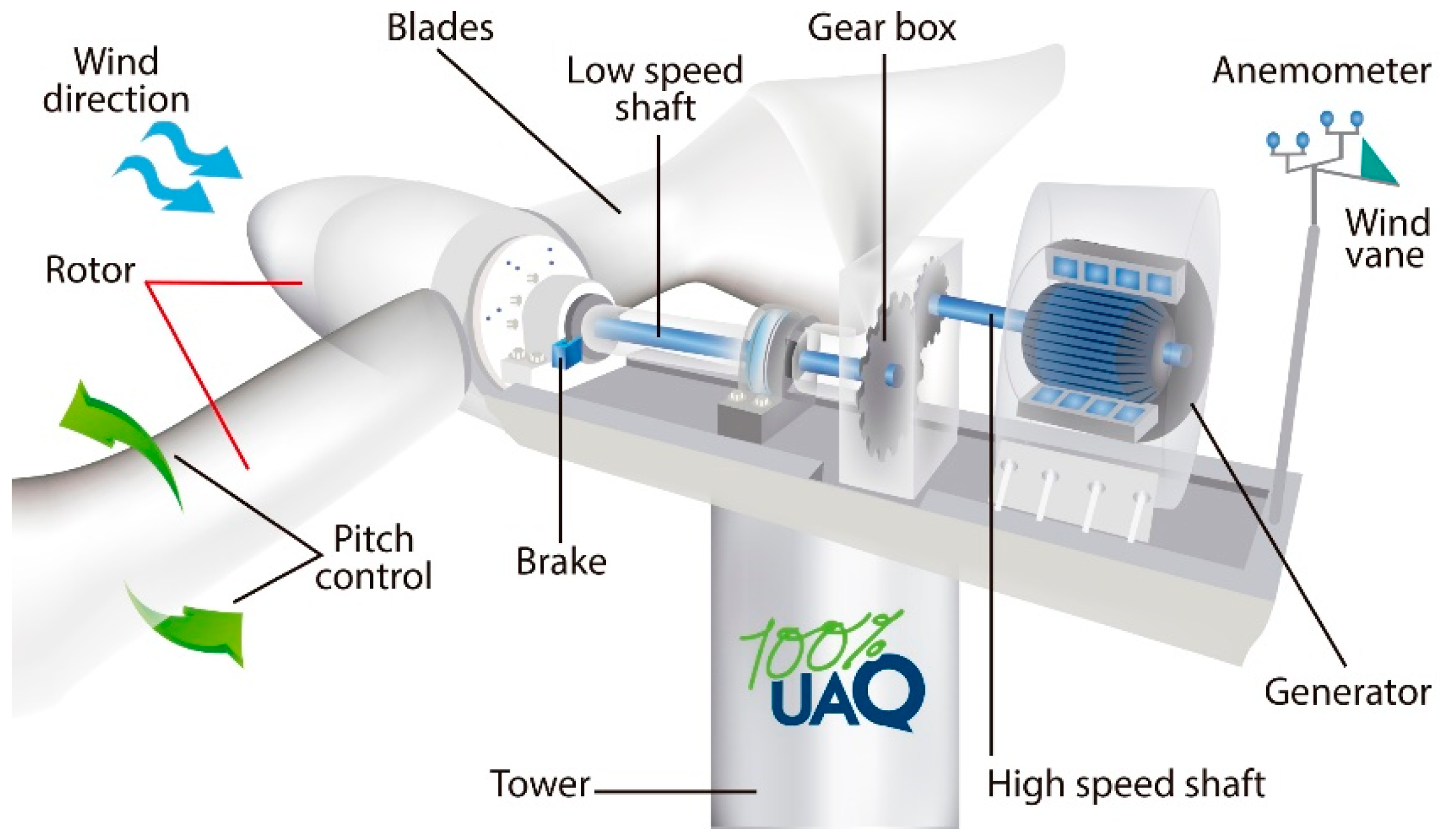
The turbines are composed of three main parts, the rotor of blades that converts the kinetic energy from the wind to mechanical energy, the gearbox that multiplies the speed of the rotor and transmits it to the rotational shaft of the generator, and the electric generator [
28]. Additionally, some systems convert AC to DC using a rectifier and convert DC back to AC to match the frequency and phase of the network [
29]. A diagram of a wind turbine is shown in
Figure 1.
2.1. Mathematical Model
The mathematical model of the wind turbine is made by subsystems, the aerodynamic model of the rotor, the mechanical model and the electric model of the generator are determined.
To perform an aerodynamic analysis of how to extract the maximum power of the wind that passes through a turbine, the wind that crosses the sweeping area of the rotor is determined. The rotor power
Protor extracted by the blades is described with the Equation (1) [
30].
where the wind density is
ρ, A is the swept area,
V is the wind speed before the turbine.
Cp is the power coefficient, which can be expressed in approximate method depending on tip speed ratio
λ, that is the ratio between the tangential speed of the tip of a blade and the actual speed of the wind and on the pitch angle of the blade
β, based on the characteristics of the turbine [
31,
32].
Cp is defined as:
where:
Ω is the rotation frequency in rad/sec,
n is the speed of rotation in rpm and
R is the radius of the rotor. Once the
Cp has been calculated, it is possible to determine the torque of the rotor
Trotor with the following equation: [
33,
34].
where torque coefficient
Ct is defined as:
The mechanical system transmits the mechanical torque of the rotor, multiplies the speed of the rotor shaft
n times towards the generator shaft. The mathematical model of the mechanical system can be simplified throughout the system into a two masses model, which is the most common model for wind turbine transmissions and can be used without losing accuracy [
35,
36]. In the mechanical model, the aerodynamic torque of the wind turbine rotor and the electromechanical torque of the generator act in opposition to each other and are the inputs to the model, while the rotation speeds are the output [
37,
38]. The mathematical model is represented by the Equations (7) y (8). The model of two masses proposed by [
19] is shown in
Figure 2.
where the inertial constant depends exclusively on the geometry and distribution of the mass of the element. The elasticity between adjacent masses is expressed by the spring constant
ksh and the mutual damping between adjacent masses is expressed by
dsh [
36,
37].
θrotor is the rotor angular position and
θgen is the generator angular position.
Hrotor and
Hgen are the rotor inertia and generator inertia, respectively.
The inertial moments
Hrotor and
Hgen are calculated according to:
Jgen is the inertia of the generator and is regularly provided by the manufacturer. In the case of the inertia of the rotor
Jrotor it can be approximated according to:
where
mr represents the mass of the rotor (includes the mass of the blades).
The generator is electromechanical equipment that converts mechanical power into electrical power, uses a stator and a rotor. The stator is a housing with coils mounted around it. The rotor is the rotating part and is responsible for producing a magnetic field, it can be a permanent magnet or an electromagnet. When rotating, its magnetic field is induced to the stator windings causing a voltage at the stator terminals [
28]. According to the needs of the market, the synchronous permanent magnet generator (PMSG) is used commonly because of its adaptation to variable-speed turbines [
38]. The PMSG has a high efficiency since its excitation is provided without any power supply. It requires the use of an AC/DC/AC power converter to adjust voltage and frequency to the supply network [
39].
For the mathematical modeling of a PMSG, the three phases are transformed into an equivalent of two axes. This is because each one acts in a defined geometric space of the air gap. With the direct axis (
d) in phase with the winding of the rotor field and the quadrature or displacement axis (
q), 90 electrical degrees forward in a synchronous rotating
d-q reference frame. Magnetic flux waves due to the winding of the stator are presented in two sinusoidal waves distributed rotating with a synchronous speed such that one is the maximum point on the axis
d, and the other is the maximum point on the axis
q. The stator output voltages
d-q of this generator are given respectively by Equations (12) and (13) [
40].
where
L are the inductances of the generator,
R is the resistance and
I is the currents in the axes
d and
q, respectively.
φf is the permanent magnetic flux.
ωgen is the rotation speed of the PMSG.
Pp is the number of pairs of poles. Electromechanical torque
Tgen can be express as:
ωref is the reference speed to control the speed of the generator shaft. The model reference speed is normally 120% but is reduced for power levels below 46% [
41]. This behavior is represented in the model by using the following equation:
P is the electric power. In the controller, the speed reference is not directly a function of power, but the overall effect on the speed/power relationship is similar.
2.2. Control System
The complexity of modern wind turbines forces its control systems to ensure safe and efficient operation. The objective of control systems is to ensure a continuous supply of energy to the grid, maximize energy production, and mitigate dynamic and static mechanical loads. The pitch angle of the blade, the torque of the generator, and the frequency on the grid are the main parameters that must be controlled [
42].
The definition of the control objectives depends on the operating regions of the wind turbine. These are closely related to wind speed, and one can identify four operating regions according to the wind speed. Region I represents the wind speed at which the rotor cannot move, so the rotation speed is zero. When the rotor begins to rotate, enters region II, this region is limited by the starting speed and wind speed where the generator rotates at its nominal speed. The objective of control in this region is to maximize energy production through MPPT strategies. Region III starts from the nominal speed to the stopping speed, which is the design speed limit and is required to stop rotation for safety. To maintain the constant nominal rotation speed, the pitch control is used. However, MPPT control is also used in this region to smooth out abrupt changes in wind speed, where the mechanical restrictions of the pitch system do not allow a rapid response. Finally, region IV is where the wind turbine must be stopped even with a mechanical brake [
42,
43].
The pitch control system in a wind turbine is used to regulate the power of the rotor, control its speed of rotation and stop the rotor out of the action of the wind. In region III, during high-burst winds, it is necessary to control the rotation speed of the rotor to protect the generator and electronic equipment from overloads. The inertia of the large rotors in acceleration and deceleration must be considered to decrease the dynamic mechanical stresses in the blades and the tower. The speed of rotation is variable with the angle of incidence. This angle is formed between the line of direction of the wind and line that marks the side of the blade. This angle of incidence is increased to take advantage of the wind speed and is reduced when the speed of rotation increases. The adjustment of this angle is made to keep the power captured by the wind constant. The angle of incidence changes with the pitch angle, which is the angle of rotation of the blade with respect to its axis. Consequently, the power coefficient is affected by the evolution of the pitch angle [
44].
In
Figure 3, the power coefficient curves with different values of the pitch angle are shown. When the angle value increases, the power coefficient decreases, the captured wind power is reduced, and there is a reduction in the rotor velocity.
The control model used is a PI controller with feedback [
17]. The purpose of a feedback control system is to reduce the error
e(k) to zero between the variable to control and its reference value as quickly as possible. The error is expressed as:
The pitch control signal u(t) to the plant is equal to the proportional gain Kp times the magnitude of the error plus the integral gain Ki times the sum of the errors of samples, k is the sample number from a total of ksim samples.
To select the parameters of the
Kp and
Ki controller that comply with the presumed behavior of the system, it is proposed to follow the tuning rules of Ziegler–Nichols [
45] based on the experimental responses to a step input. However, there may be a large overshoot in your response that is unacceptable, so a series of fine adjustments is necessary until the desired result is obtained.
The pitch angle command activates a mechanic system back and forth for the pitch control system. The faster the settling, the lesser the mechanical stress on the turbine and structure.
3. Intelligent Search Algorithms Teaching–Learning
Teaching–learning-based optimization (TLBO) is based on the teaching and learning process in a classroom. In each generation, the best candidate solution in the population is considered the teacher, and the other candidate solutions are considered learners. The learners mostly accept instruction from the teacher, but also learn from each other. The score of an academic subject is analogous to the value of an independent variable or candidate solution feature [
46,
47]. The steps of the algorithm are described below.
Step 1: Define the optimization parameters.
Population size (Pn),
Number of generations (Gn),
Number of design variables (Dn),
Limits of design variables (LU, LL).
Objective function f (x)
Define the problem: Maximize f (x), minimize f (x).
X is a vector of design variables such that:
Step 2: Initialize the population.
Generate a random population according to the size of the population and the number of design variables. For TLBO, the size of the population indicates the number of students, and the design variables indicate the subjects that are offered. This population is expressed as:
Step 3: Teacher Phase.
Calculate the average of the population, which will give the average for the subject as:
The best solution
Tf(x)max,min will be teacher
Tteacher for that iteration
The teacher will change the mean of MD to Xteacher, which will act as a new average for the iteration.
The difference between two means is expressed as:
r is a random number in a range [0,1]. The value of
TF is selected as 1 or 2. Teaching value that decides the value of the mean to be changed. No design value is random, given by the algorithm:
The difference obtained is added to the current solution to update its values using:
Accept Xnew if you give the function a better value.
Step 4: Learning Phase.
A student interacts randomly with other students. A student learns something new if the other student has more knowledge than he does. Randomly select two learners Xi and Xj, where i ≠ j.
The knowledge of both students is compared.
When all the students have interacted, accept Xnew if you give the function a better value.
Step 5: Termination criterion.
Stop if the maximum generation number is reached, otherwise, repeat from step 3.
Figure 4 shows a flow diagram of this algorithm.
This optimization method was selected since it converges on a solution in a shorter time compared to other known algorithms, this is because it uses the best iteration solution to change the optimal reference solution existing in the population, in addition to using a minimum of computer resources since it only uses simple arithmetic operations such as sums and divisions.
A performance analysis of the proposed algorithm was developed and compared with other intelligent search techniques such as genetic algorithm (GA) [
48], simulated annealing (SA) [
46], ant colony optimization (ACO) [
46], differential evolution (DE) [
46], and firefly algorithm (FA) [
46], particle swarm optimization (PSO) [
26], moth flame optimization (MFO) [
27]. Test functions (28) suggested in [
48] were used.
This equation was selected due to its similarity to the objective function, since it has higher and non-linear terms of order, in addition to being initialized at a starting point (first solution). Another important feature is the mathematical minimization problem with two variables, as in the application of the wind turbine, it is necessary to find the value of the variables
kp, ki that minimize the error in the controlled variable.
Table 1 lists the specifications with which the test was performed.
From this analysis, the computation time for the search for each optimal solution was obtained. The computational resource was an HP Workstation i-7 processor and 32Gb RAM, 64bit, for all tests.
Table 2 shows this comparison, where it is evident that the teaching–learning algorithm obtained a better performance.
According to the results presented in the previous table, the TLBO algorithm had better results in the computation time and obtained a minor error in relation to the exact known solution, this is due to the advantages of the algorithm. The advantages of the algorithm are that it does not require any parameters to adjust, which simplifies the implementation, uses the best solution of the iteration to change the existing solution in the population which increases the convergence rate. TLBO does not divide the population as other algorithms do, but it uses two different phases, the "teacher phase" and the "student phase", so that new random solutions can be evaluated, and no time is spent evaluating the same solutions among themselves. The disadvantage is that no measures are taken to handle the limitations of the problem. Solution selection is only done in a heuristic way by comparing two solutions.
4. Methodology
The proposed methodology for the optimization of the use of wind energy for the generation of electric energy through a PI controller with variable gains includes the following steps. First, know the available wind resource by making a preliminary study of the historical records of the climatic conditions at the installation site, as well as having physical knowledge of the wind turbine. This will allow us to characterize the wind behavior statistically to know the limits of wind conditions. Second, design a PI controller for the pitch angle, tuned for a response speed according to the sensitivity presented by the system, in a range of nominal wind speed values. This allows us to keep the controller in a stable state with typical winds. Third, once the response values of the controller are in their stable state, the limitations and operating ranges of the controller are proposed to establish the optimization parameters of the TLBO algorithm, which will improve the response of the controlled when atypical winds occur, such as bursts or turbulence.
4.1. Wind Resourse and Wind Turbine Specifications
The wind turbine used for experimentation is located at the UAQ, airport campus, road to Chichimequillas s/n, Ejido Bolaños, Querétaro, Qro. Z.C. 76140. The geographic location 20°37’24.1″ North and 100°22’06.0″ West and an altitude of 1969 m a.s.l.
Figure 5 is an image of the airport campus of the autonomous university of Queretaro, where the wind turbine and the adjacent buildings are shown.
This research incorporates aerodynamic modeling based on a meteorological study with data collected in the weather station #76628 SMN-CONAGUA network, located in the place, with stored data from the last five years. The average annual recorded speed is 3.9 m/s, and the range of recorded wind speed values is between 0 and 15.69 m/s.
This wind turbine is a NACA 6812 airfoil with two blades of 6.4 m in length and 1.2 m at their widest point, constructed of fiberglass and polyester resin, weighing 260 kg each. The height of the tower is 18 meters. There is a multiplier box with a ratio of 1: 2.1, and a permanent magnet generator with a rated power of 14 KW at 14.6 rad/s speed.
4.2. Pitch Control
To form the plant to be controlled, the different mathematical models were integrated, in the dynamic model, the input data is wind speed that is the disturbance of the system and the pitch angle that is a variable that is originated in the controller, the output is the mechanical torque of the low-speed shaft. The information we obtained from the mechanical model is the rotation speed of the shaft at the output of the multiplier box or high-speed shaft. In the generator model, the generated electrical power was calculated and due to its electromagnetic properties, the torque of the generator, which in turn is a force opposing the rotor torque. The controlled variable is the speed of rotation of the rotor. The limitation in this control model is the speed of rotation of the blade, the maximum speed is 1.5 °/s because a 0.5 HP motor mechanically spins a reducer with a 60:1 ratio, which increases the torque to counteract the effects of air on the blade, but greatly decreases the speed. The control model that describes the operation of the systems is shown in
Figure 6.
The controller gains were established empirically by performing various simulations in MatLab-Simulink R2018b V9.5.0.944444 program. The wind speed from 0 m/s to 15.69 m/s, maximum wind speed at the site, was used as an input variable. The setpoint for the controller is the rotation speed of the nominal generator shaft of 14.6 rad/s.
The system is limited to a wind speed between the starting speed and the cutting speed, within these limits the system must be stable. Tuning was performed by applying a step input with the value of the nominal wind speed, which means the maximum value of an accepted disturbance. With respect to the sensitivity of the system at different wind speeds, the system must not have an over impulse greater than 20%, so a range of PI gains from the controller that were within the limits of this condition was obtained. Therefore, the controller can minimize the error of the controlled variable under these disturbance conditions and ensuring that the system is stable. The gain values obtained using the Ziegler–Nichols method for PI controller and experimentally adjusted are Kp = 2.2 and Ki = 0.1, gain values Kp = 10 and Ki = 0.01 were also obtained for a system with 20% overshoot and Kp = 1 and Ki = 1 for an overdamped system.
Figure 7 shows the behavior of generator shaft speed with the gain values obtained for a stable system, a system with overshoot, and an overdamped system.
Figure 8 contains the pitch angle movement for all cases.
4.3. TLBO Algorithm Application.
According to the analysis performed in the process of tuning a PI controller, in point 4.2, the optimization parameters were defined:
Population size (5), a small number of initial random solutions for each design variable is proposed, which reduces the convergence time, in addition, there is the possibility of increasing the search space since the switching between student-teacher phase is carried out faster and new random solutions can be evaluated and no time is spent evaluating the same solutions among themselves.
Number of generations (100), the maximum number of interactions was proposed after verifying that for this case study the convergence of a solution was obtained around 50 interactions.
Termination criteria: If there are more than 25 interactions without having a better profit proposal, the search process ends.
Design variables (Kp, Ki), controller gains.
Limits of design variables, 0 ≤ Kp ≤ 10, 0 ≤ Ki ≤ 1 the limits were established based on knowing the optimal values of the design variables for the overshoot system and overdamped system, for nominal wind speed ranges.
Objective function,
f(x) = mathematical model, this model was described in
Section 2 of this publication.
Define the problem: minimize e(k), the objective is to find a solution that reduces the error between the nominal rotation speed of the generator shaft and the measured speed.
The calculation of the new gains was made every second, since the execution time of the algorithm was less than this time. MatLab-Simulink R2018b V9.5.0.944444 program was used to run the algorithm on an HP Workstation i-7 processor and 32 Gb RAM (64 bit). The experimentation was performed by programming a PIC16F87A using the Dev C ++ V5.0.0.4 software. The control model proposed proportional-integral with teaching–learning based optimization (PI-TLBO) is shown in
Figure 9.
5. Results
According to simulations performed to obtain the empirical values of the
Kp and
Ki gains, a maximum power factor of 4.47 and the wind speed of 6 m/s were determined under ideal conditions and shaft generator nominal speed of 14.6 rad/s. However, the magnitude of the change in wind speed makes the system unstable, since the thrust force provides different acceleration to the rotor rotation. Therefore, a PI controller with variable gains was proposed to obtain different response times in the controller and soften these changes. The effectiveness of a pitch control using the PI-TLBO algorithm is examined in real operating conditions. The recorded wind speed values are shown in
Figure 10.
The search time for each value of Kp and Ki is in a range of 0.4 and 0.75 seconds depending on whether the algorithm makes all interactions or not, so a variable adjustment is made every second. With this result, the convergence speed of the algorithm can be highlighted, where unlike other optimization algorithms, it uses the best iteration solution to update the value of the existing solution, in addition to reducing the processing time since they are only used simple arithmetic operations such as sums and divisions.
Figure 11 shows the development of the algorithm in (a) there is an error of the variable that decreases according to better values of
Kp and
Ki, in (b) and (c) we observe how the values
Kp and
Ki change respectively.
The results of the experimentation show that the algorithm of optimization of gains
Kp and
Ki generate a better performance of a PI controller. In
Figure 12, a comparison is made between the response of a PI controller and a PI-TLBO controller, the speed obtained from the generator shaft behaves more smoothly and close to the nominal speed, which represents a reduction in fatigue in the wind turbine structure and lower saturation in the PMSG.
It is also observed that the response of the PI_TBLO controller has a minor overshoot in the optimization range, the stabilization period is also reduced when a major disturbance occurs. Therefore, it can be suggested that after the TBLO optimization process for calculating the gains of the PI controller, the proposed control model is expected to control the pitch angle under various disturbances.
Figure 13 shows the movement of the
Kp and
Ki gains throughout the experimentation.
It is important to note the efficiency of the algorithm, a series of simulations were performed to validate the repeatability finding small variations in the response of the controller, this is due to the randomness of the data to generate new responses in the teacher phase. However, any of the responses of the PI-TLBO controller obtained better performance than that of the PI controller, this can be seen in
Figure 14.
6. Discussion
The use of dynamic models to simulate the aerodynamic behavior of the system allows to know the behavior of a wind system, however, in this type of systems, it is not necessary to know the behavior of the wind speed or the magnitude of its changes that would be the variable input. The multiple variables involved in the output variable make the system nonlinear, which also becomes a problem to calculate the ideal parameters of the controller. That is why a controller that adjusts to various changes in the system variables is proposed, this controller is automatically adjusted by an optimization algorithm based on teaching–learning, which gave the system stability since the controller adjusted its control response according to wind conditions. A better response was obtained by constantly adjusting the controller with a method of close solutions to the optimal one, than by applying a single optimal deterministic method. This is since a suitable adjustment of the controller is required to the sensitivity of the system, since the closer it is to nominal wind speed, the system is more sensitive to wind changes, not so when the system is below the nominal speed.
A PI controller with dynamic gain adjustment and not a PID was used because the differentiation reacts as fast as the input changes with respect to time, the differentiation acts towards the future anticipating the overshoot trying to offer a response according to how quickly it increases or the input signal decreases, however, when applied in a system of dynamic gains, differentiation caused oscillations in the system, this is because it is not necessary to anticipate the future since the calculated gains act in the present. That is why it was decided to use only a PI controller, getting good results.
The presented control system affects the angle of inclination to limit wind energy, however, additional subsystems suggest the implementation of speed control to obtain an optimal electrical frequency and transfer the total electrical energy to the electricity grid.
It is convenient to use new forms of intelligent control, such as fuzzy systems, neural networks, and genetic algorithms. With this type of control, a predictive model for the expected climate would be achieved and with that would anticipate a better control response, which would reduce the frequent stops and starts of the system. In addition, the algorithms of these systems are programmed according to the knowledge and experiences that a human expert would have in the field. This is very useful since you cannot have an exact mathematical model of the meteorological parameters.
It is necessary and essential to prepare more professionals in universities with this new approach, which consists in considering the design of the wind turbine and its integration with the environment.
7. Conclusions
The use of wind energy in places where this natural resource is available should be an alternative for the generation of electrical energy, since it does not harm the environment and the wind does not end. There are places of difficult access due to their complicated orography surrounded by mountains where the wind is turbulent with various changes in wind speed.
A small deviation in the wind speed causes a large deviation in the output power of the wind turbine rotor due to the association of cubic links between these two parameters. This, in turn, translates into system vibration, mechanical fatigue, and an acceleration in the rotation speed that exceeds the nominal rotation speed of the generator.
Pitch control is the movement of the blades to receive wind power, conventional PI control is efficient in a stable state, but not in sudden changes in wind speed. This article proposes a new method of effectiveness for a PI controller based on the optimization of the gains used, which represents a better control response in different wind speed ranges. The proposed PI-TLBO algorithm proved to be efficient, since better performance was obtained compared to a conventional PI, it proved to be repetitive even though, in the teacher phase, the algorithm uses a random choice of parameters to generate new solutions. The algorithm has a rapid calculation speed due to the simplicity of its operations.
In general, with the PI-TBLO controller there is a lower overshoot and that the stabilization period is also reduced when disturbances occur, therefore it is highly efficient to control the pitch angle of a wind turbine under various atypical wind disturbances such as bursts and turbulence, reducing the transient effects of the controller and, consequently, the energy consumption in the actuator. Moreover, it was evident that the error between the nominal rotation speed of the generator shaft and the measured speed was considerably reduced, therefore, the generator is prevented from having losses due to magnetic saturation. According to the above, it can be ensured that the generation of energy in a wind turbine is increased with the use of an optimized PI-TLBO control algorithm to position the pitch angle.
The limitation of this work was the reaction speed of the mechanical system, the controller proved to be highly efficient, however, with extreme wind gusts, the actuator did not have enough speed to adjust the angle. An improvement to the design of the control model is the location of the wind speed measurement system, placing it at a specific distance, where the bursts of time are detected in advance and the controller can give a timely response, thereby the control transients that make the system unstable would be further reduced.
The use of algorithms that efficient the use of wind turbines is key to boost the use of wind energy with small wind turbines where the wind is not stable and the use of large commercial wind turbines is not possible or profitable.

 ,
, 


