The Spillover Effect of Geotagged Tweets as a Measure of Ambient Population for Theft Crime


1
Department of Geography and GIS, University of Cincinnati, Cincinnati, OH 45221, USA
2
Carl H. Lindner College of Business, University of Cincinnati, Cincinnati, OH 45221, USA
3
College of Civil Engineering, Nanjing Forestry University, Nanjing 210037, China
*
Author to whom correspondence should be addressed.
Sustainability 2019, 11(23), 6748; https://doi.org/10.3390/su11236748
Submission received: 25 October 2019
/
Revised: 21 November 2019
/
Accepted: 26 November 2019
/
Published: 28 November 2019
(This article belongs to the Section Sustainability in Geographic Science)
Abstract
:As a measurement of the residential population, the Census population ignores the mobility of the people. This weakness may be alleviated by the use of ambient population, derived from social media data such as tweets. This research aims to examine the degree in which geotagged tweets, in contrast to the Census population, can explain crime. In addition, the mobility of Twitter users suggests that tweets as the ambient population may have a spillover effect on the neighboring areas. Based on a yearlong geotagged tweets dataset, negative binomial regression models are used to test the impact of tweets derived ambient population, as well as its possible spillover effect on theft crimes. Results show: (1) Tweets count is a viable replacement of the Census population for spatial theft pattern analysis; (2) tweets count as a measure of the ambient population shows a significant spillover effect on thefts, while such spillover effect does not exist for the Census population; (3) the combination of tweets and its spatial lag outperforms the Census population in theft crime analyses. Therefore, the spillover effect of the tweets derived ambient population should be considered in future crime analyses. This finding may be applicable to other social media data as well.
1. Introduction
Census population has long been utilized as one of the most important factors in analyzing issues related to crimes in the fields of criminology, sociology, economics and many more [1,2,3,4,5,6]. However, it is generally recognized that the vast majority of the available Census population data represent the residential population and cannot capture the ambient population distribution [7,8,9]. Consequently, using the Census population alone to analyze the crime would be potentially problematic and biased sometimes [6,9,10,11,12,13,14,15]. Therefore, it is pressing to discover other complementary indicators of the ambient population with the high spatio-temporal resolution to advance the understanding of crime patterns.
Due to its timely availability and free accessibility, tweets have been widely used by researchers to model patterns of the ambient population [16,17,18]. Sims and colleagues (2017) use the Twitter posts and Facebook check-ins across a 24-hour period for football game days at the University of Tennessee, Knoxville, during the 2013 season to model the dynamics of the population distribution during the special event. After comparing the population distributions for game-hours and non-game-hours with the social media data, they successfully test the reliability of using social media data to improve the dynamic population distribution model [19]. Patel and colleagues (2017) collect two months of geotagged tweets in Indonesia in 2013 and use its density as a covariate layer to map the distribution of the population. This approach significantly increases the population mapping accuracy, argued by authors [20]. Therefore, it is obvious that geotagged tweets can be a significant factor for the location-based services because of its promise for more dynamic population distribution detection, especially when people are not at their residential locations [17,18,19,20,21].
In the field of environmental criminology, it is common knowledge that most of the criminal actions require the convergence of the motivated offender, the suitable target and the absence of the capable guardian in space and time. This routine activity approach highlights the importance of the dynamic population distribution on the crime. The development and rapid change in human society encourage people to have more routine activities away from their homes [22]. The increased mobility and the mobile range will certainly change the dynamic distribution of the population, which in turn, influences the crime pattern [23,24,25,26,27]. Moreover, Crime Pattern Theory suggests that both offenders and victims have their own behavior patterns, consisting of the same or different anchor locations. The crimes are more likely to happen in the intersected anchor locations of their activity spaces [28,29,30,31,32]. These anchor locations can be crime attractors, which create well-known criminal opportunities to which motivated criminals are attracted; or crime generators, which attract a large number of people who have no intention to commit any crime [29,30,31]. It is clear that crime attractors and generators have great potential to attract people; however, the number of people attracted to each attractor/generator is hard to discern from the Census data. The spatio-temporal information embedded in the Twitter posts (also known as tweets) can be a potential asset to the crime pattern analysis by acting as an ambient population index. It has the potential to capture dynamic population distribution. Moreover, crime data have a high spatio-temporal resolution, so is the tweet. In contrast, Census data in the US tend to have a low spatio-temporal resolution. Incorporating tweets should better explain crimes due to matching resolutions.
There have been a number of studies that touched on the relationship between tweets and crime. Gerber (2014) uses the semantic analysis to extract the topics of tweets and calculates the relative strength (weight) of individual topics as independent variables, along with the historical crime data to predict future crime in Chicago. The result suggests that the addition of Twitter-derived features improves prediction performance for 19/25 crime types than the model of solely historical crimes [33]. His approach adds 300–900 topics (each topic is an independent variable, and these topics are not necessarily related to crime) into the prediction model, which would almost surely increase the performance of the prediction model. The theoretical foundation of this research is relatively weak since it does not introduce sufficient criminology theory to justify the crime prediction model. In spite of this obvious disadvantage, this study demonstrates the benefits of tweets for crime prediction. Other scholars also try to explain the crime distribution with geotagged tweets. Bendler and colleagues (2014) use the amount of point of interest (POI) as the independent variable to simulate crime incidents happened in San Francisco from August through October of 2013. Then they add the count of tweets into the model and argue that the performance of the simulation model increases [34]. Ristea and colleagues (2017) try to use tweets count as an explanatory variable to assess the crime-tweets relationship, and they find the significant correlation between the two in aggregated crime types, anti-social behaviors, and other thefts [35]. However, none of these includes any socio-economic variable as controls when modeling the crime. Therefore, they cannot answer whether the relationship between tweets and crime is spurious. Three UK scholars derive “broken window” indicators (e.g., neighborhood degeneration) from the content of tweets [36]. They add the frequency of Twitter posts and the count of tweets containing “broken window” indicators into a model, with the control of necessary socio-economic variables, to simulate crimes that happened in 28 London boroughs from August 2013 to August 2014. They argue that naturally occurring social media data may provide an alternative information source on the crime problem [36]. By using a sample of tweets in the Southern California region from May 2015 to December 2015, Hipp and colleagues (2018) also suggest that this data source can help explain the existence of crime [15].
The aforementioned studies use the count of geotagged tweets or its transformation (e.g., natural logarithm) as a replacement of the Census population in their crime models with the presumption that these tweets can provide a better estimate of the ambient population than Census population [14,15]. However, how “better” can this new indicator of the ambient population be having not been thoroughly measured using the solid statistical method. Moreover, though a body of literature has demonstrated that the count of tweets is an appropriate indicator of the ambient population, should it serve as a replacement or complement of the residential population in the crime model is not tested. In addition, the mobility of Twitter users and the contents of tweets not being restricted to the tweets’ location may suggest that tweets, as a measure of the ambient population, may have a spillover effect on the neighboring areas. However, such effect has never been tested for the tweet-crime relationship.
The spillover effect of tweets is important because it serves as an indicator of the ambient population, which contains mobility information that is not available in the Census population [8,14,37]. Moreover, the reason for using the ambient population in the model is to capture the non-residential population in the neighborhood. A Twitter user may tweet at the residential neighborhood, at the adjacent neighborhoods, at work location or other anchor locations of the routine activities. Consequently, embedded mobility information can be revealed by tweets. As crime is closely linked to the actual pattern of the ambient population [8,14,37], a measure of the ambient population’s spillover effect should help in the explanation of crime patterns.
One of the approaches for representing this spillover effect is through the use of spatial lag of tweets based ambient population. By its definition, the spatial lag is a weighted average of one variable at “neighboring” locations, which can account for its spatial autocorrelation (i.e., the value of a variable in one unit is correlated with the values of the same variable in this unit’s neighbors) [38,39,40]. The spatial lag regression model has been used in a few environmental criminology studies, by introducing the spatial lag of crime as an explanatory variable [38,41,42]. However, the spatial lag of the ambient population has not been included in any crime model to account for its spatial spillover effect. Given the potential importance of this spillover effect of the ambient population on the crime, this gap should be filled.
The aforementioned research gaps motivate us to tackle the following research questions: (1) Should tweets based ambient population be considered as a replacement or a complement of the residential population in theft crime models? (2) How does the spillover effect of tweets based ambient population contribute to the explanation of theft patterns? (3) Do tweets explain theft patterns better than the residential population?
2. Study Area and Data
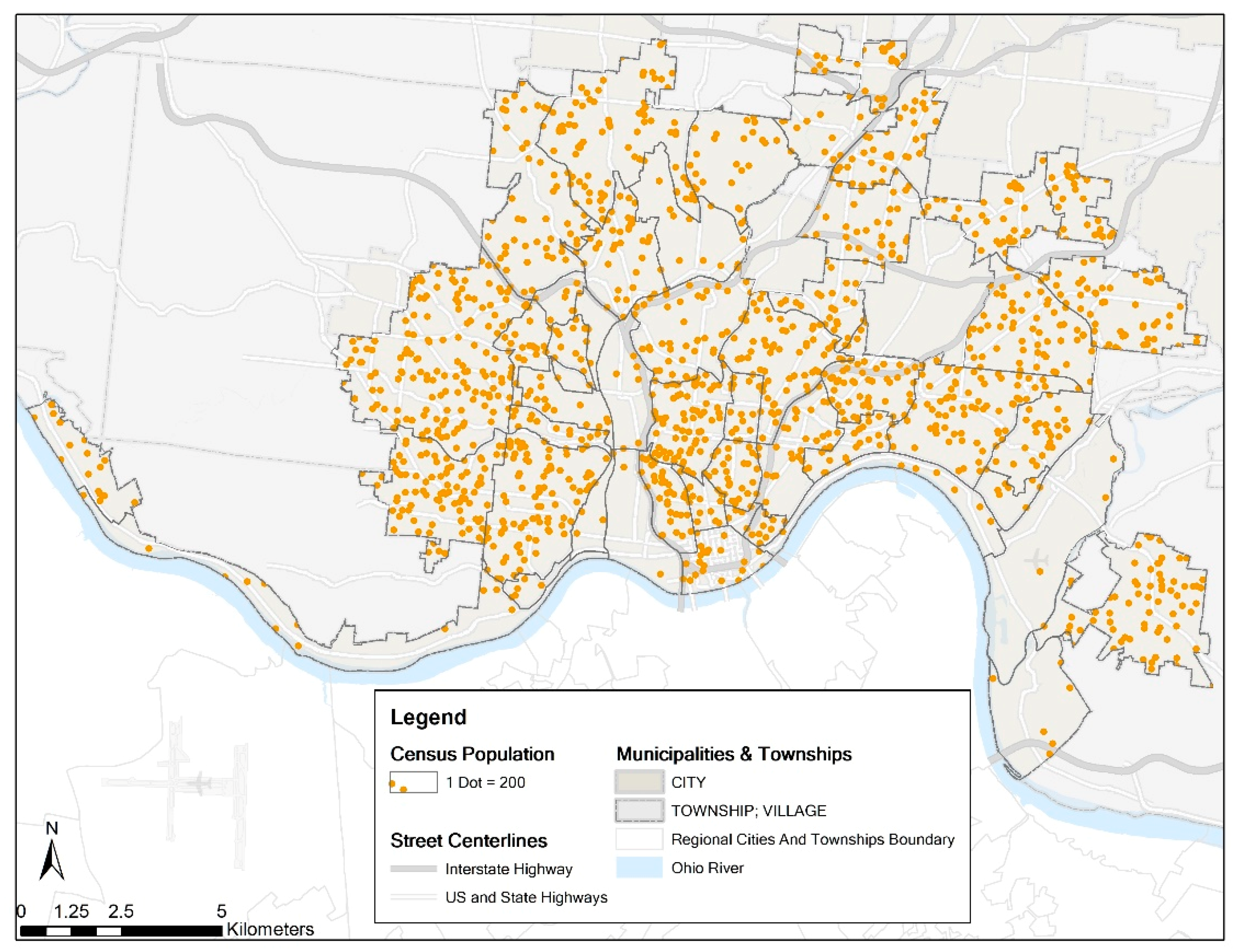
The study area of this research is the City of Cincinnati, the core of the Greater Cincinnati Metropolitan Area. Cincinnati is within Hamilton County, OH. The University of Cincinnati is located in this city. Based on the data acquired from the Cincinnati Area Geographic Information System (CAGIS), the total area of Cincinnati is 206.01 km2, and this city is composed of 50 neighborhoods. In the year of 2013, the total population of this city was 297,444. Figure 1 shows the spatial distribution of the Census population by neighborhood. Since using choropleth maps for presenting counts is inappropriate and against the cartographic rules [43], we choose the dot density map to display the population. One dot represents 200 individuals, and the neighborhood with more dots has a larger population. This map is created with ArcGIS 10.4.1, so as to the other maps presented in this paper.
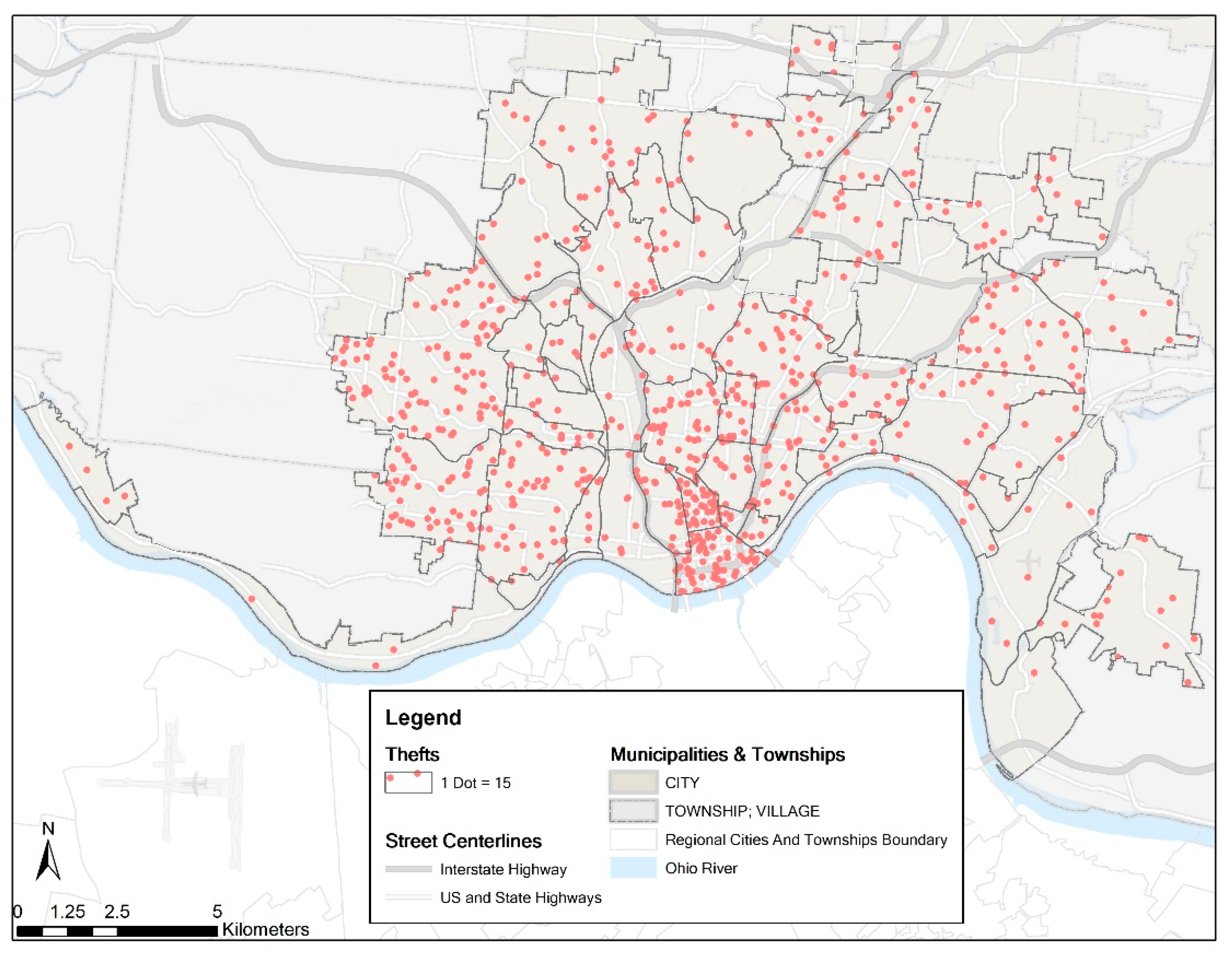
Cincinnati Police Department provides us with the theft crime incidents data for the entire year of 2013. More than 99% of these incidents (11,742/11,819) are successfully geocoded based on their addresses. Figure 2 shows the spatial distribution of the thefts by neighborhood. The dot density map is also used here, and one dot represents 15 theft incidents. The neighborhood has more dots has more thefts.
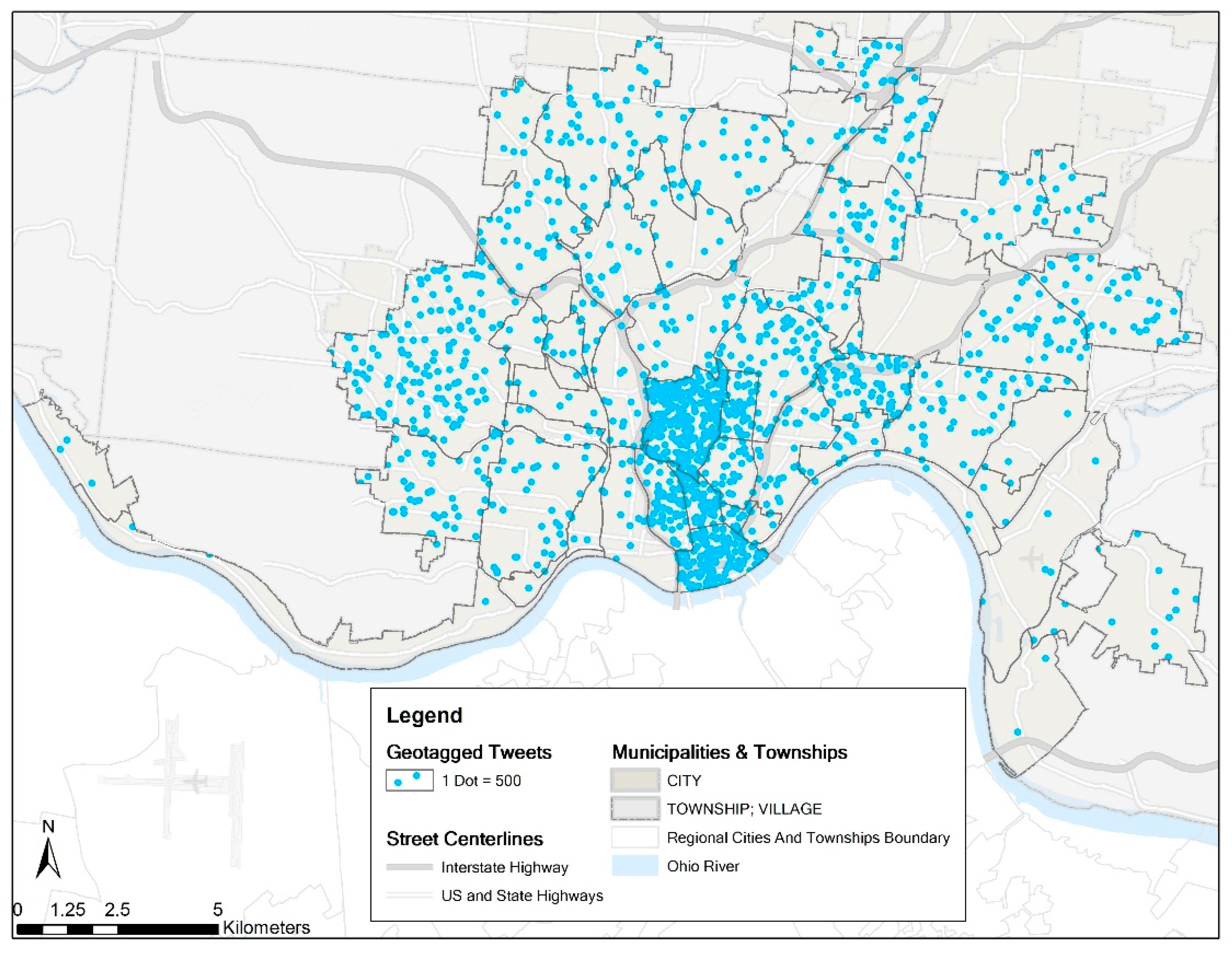
To be consistent with theft crime data, geotagged tweets (N = 778,901) in Cincinnati for the year 2013 are retrieved by adopting a Python script initially written by Henrique [44]. Unlike the Twitter Streaming API which has a limitation of time constraints (no historical tweets) and volume constraints (at most one percent of all the tweets produced on Twitter) [45], this Python script is able to mimic the tweet Search on the browser [44]. Therefore, all the public geotagged tweets in Cincinnati are retrieved. The high representativeness of this dataset is a significant advantage of our study compared with earlier ones. The anonymous user ID, date and time, latitude and longitude of the collected tweets facilitate the analysis in this study. Figure 3 shows the spatial distribution of the geotagged tweets by neighborhood in the form of the dot density map. The more points are in the neighborhood, the more the tweets are.
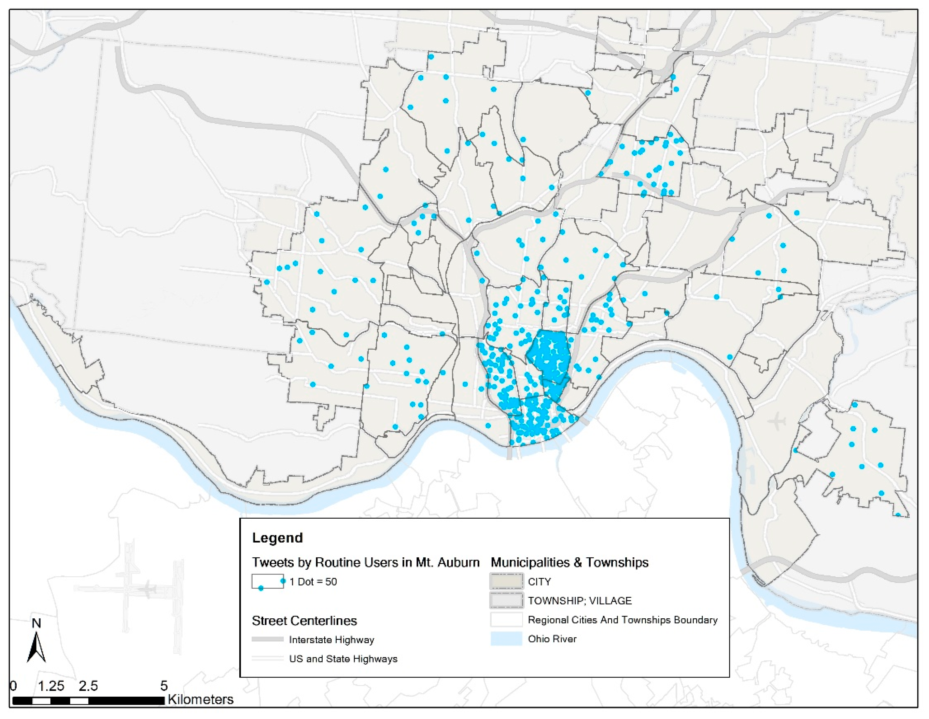
To get a sense of the plausible spillover effect of tweets, we randomly select a neighborhood, Mount Auburn. There are a total of 12,149 tweets, posted by 997 unique users in this neighborhood during the year of 2013. We select the top 35 users who posted most of the tweets (7874 in total), based on the reasonable assumption that the most important anchor locations such as home or work of these users are in the neighborhood. Then all the tweets (18,938) posted by these 35 users in the remaining 49 neighborhood areas are retrieved (Figure 4). This dot density map shows the spatial distribution of the tweets posted by these 35 users. The denser the points are, the more the tweets are in the neighborhood. It is obvious that the neighborhoods near Mount Auburn tend to have higher tweet counts, while distant neighborhoods have lower counts, indicating a distance decay pattern. A few exceptions exist because of the distribution of these users’ other anchor locations of their daily activities.
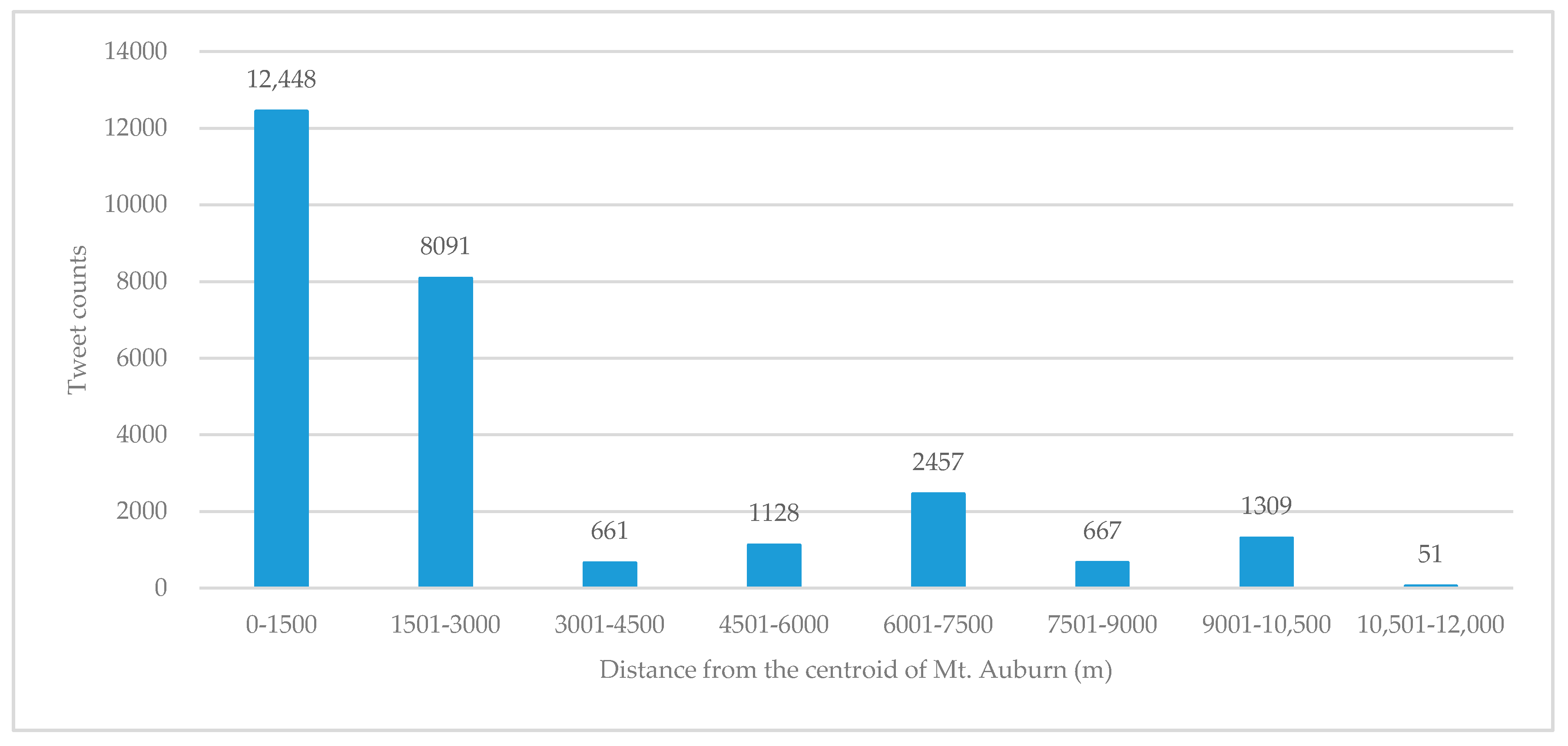
To further highlight the distance decay pattern, we also calculate these tweets’ Euclidean distance to the centroid of Mount Auburn by using ArcGIS 10.4.1. Since the dimension of Mount Auburn is about 1500 m, the interval of the bins for the histogram is set as 1500 m. Figure 5 shows the histogram of the tweets in each distance bin, demonstrating an obvious distance decay phenomenon of tweets. The revealed distance decay phenomenon serves as an empirical foundation for the hypothesis of the spillover effect of tweets on theft crime.
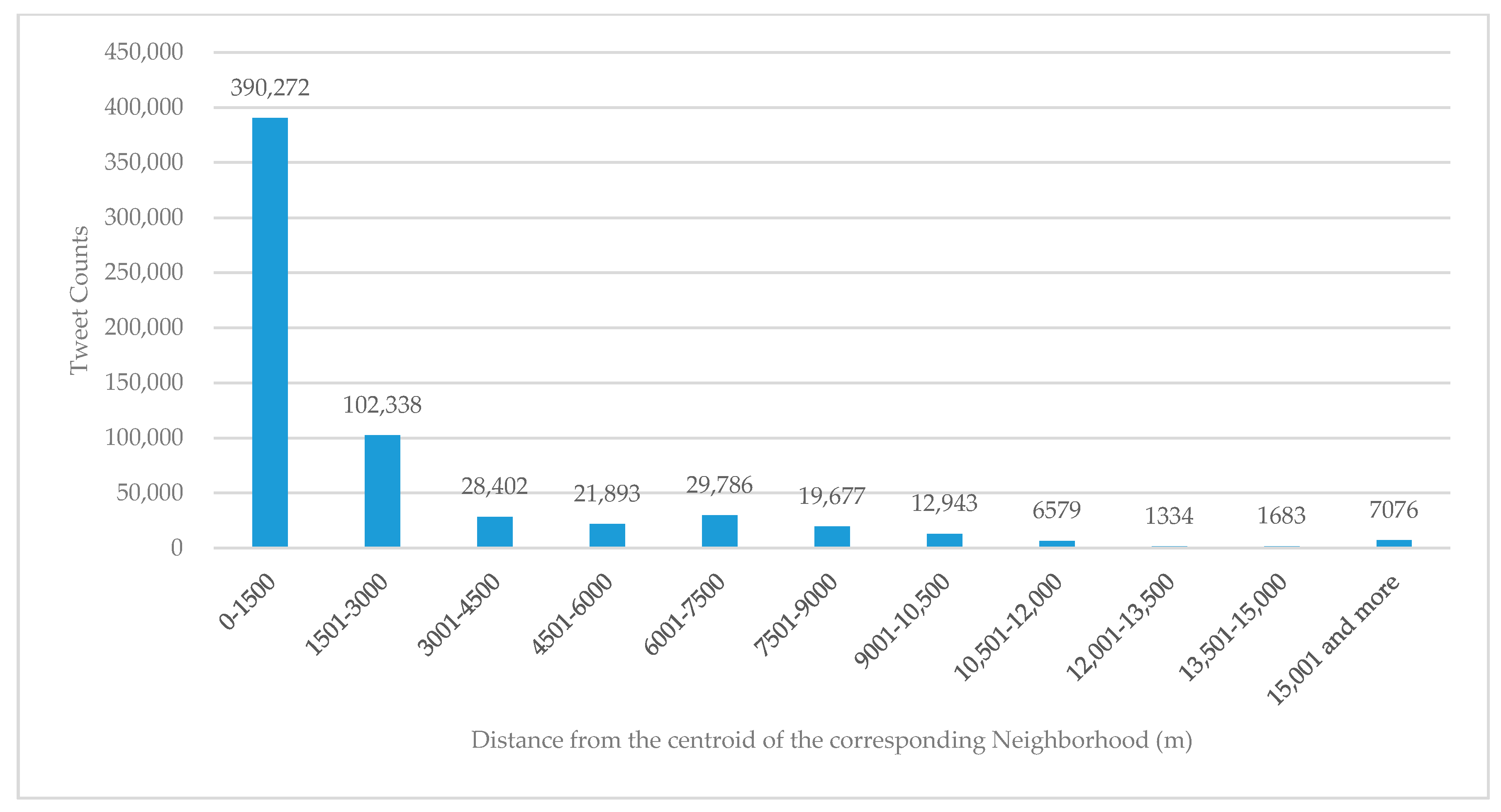
We also conduct the similar analysis on all 50 neighborhoods. Figure 6 shows the histogram of the tweets by routine users of each of the 50 neighborhoods, demonstrating an obvious distance decay from the centroid of the corresponding neighborhood. This suggests the distance decay presented in Figure 5 is not incidental. It is noticeable that the tweets count in Figure 6 drops faster than that of Figure 5. It is possible that peripheral neighborhoods experience more drastic distance decay than the ones near downtown, as the anchor points such as work locations of many users are centered in and near the downtown area.
Moreover, the tract-level socio-economic data in 2013 are retrieved from the US Census Bureau, which include total population, population under the poverty line, unemployed population, population younger than age 18, median household income, total houses, total houses currently occupied, total vacant houses, houses occupied by renters, and population in different races. These socio-economic variables are aggregated to the neighborhood-level to capture the collective characteristics of the neighborhood as proposed by existing social science studies [46,47,48,49,50]. Neighborhood-level characteristics have been tested to be related to crimes [3,51,52]. The neighborhood is also more identifiable and familiar by the local residents, media, and community councils. The results of the neighborhood-level models make more sense to the public and thus, may draw more public attention, as well as benefit the community-oriented problem solving [53,54,55]. Deriving from the social disorganization theory [56], the poverty rate, unemployment rate, the young population (<18) rate, and the median household income are used to indicate the concentrated disadvantage and inequality [48,57,58,59,60]. The housing rental rate and the housing vacancy rate are the indicators of residential instability [48,61,62]. The widely used ethnic heterogeneity index [32,63] is also added. This index is calculated as:
where B, H, W, and O are the numbers of residents of Black, Hispanic, White, and Other ethnics, respectively, who are living in the neighborhood. A score of 0 means a completely homogeneous neighborhood, while a score of 1 implies the total heterogeneity. Additionally, points of interest (POI) data, including transit stations (bus, streetcar, train, etc.), ATMs, bank branches, bars, convenience stores, grocery stores, liquor stores, movie theaters, night clubs, recreational places, restaurants and shopping malls, are collected from the Google Map. The POI variable serves as the additional control in the statistical models since these crime generators/attractors often influence crime opportunities [6,30,31,32,64,65].
3. Method
As the “Iron Law of Troublesome Places” indicates, few places are responsible for most of the crimes, and most places do not experience any crime, so the distribution of crime is always skewed [66,67,68]. Therefore, the negative binomial regression model is selected to analyze the theft crimes in Cincinnati as it does not assume homogeneity of variance [69]. It is a Poisson-based regression model suitable for an over-dispersed dependent variable and has been widely used in environmental criminology studies [32,60,69,70]. The unit of analysis is the neighborhood (N = 50).
The dependent variable is the theft count in each neighborhood. The independent variables are the Census population, the count of geotagged tweets, and the spatial lags of them. The spatial lags of the independent variables are included to address the potential spillover effect. The spatial lag of tweets in one neighborhood is calculated as the average number of all of its immediately adjacent neighbors’ tweets counts. The spatial lag of the Census population is calculated in the same manner. The software used to perform these spatial lag calculations is GeoDa 1.14 [71]. The control variables are indicators of the concentrated disadvantage (poverty rate, unemployment rate, young population (<18) rate, and the median household income), the residential instability (housing rental rate and housing vacancy rate), and the ethnic heterogeneity. The count of crime generators/attractors is added as the additional control. In order to answer all the proposed research questions, six models with the same dependent variable are generated with different independent variables and the same set of control variables by Stata 15 [72]. Table 1 shows the descriptive statistics of variables used in the models.
4. Results
Three negative binomial models are firstly generated with different independent variables: Census population (Model 1), tweets count (Model 2), and both of the Census population and tweets count (Model 3) (Table 2). The standardized coefficient (β) is calculated by multiplying the unstandardized coefficient by the ratio of the standard deviations of the independent variable and the dependent variable [73,74]. Model 1’s result shows that after controlling for the necessary socio-economic variables and crime generators/attractors, the Census population shows a significantly positive influence on thefts (β = 0.111, p-value = 0.002). This is aligned with common sense and the previous studies, as crime is a function of population distribution [4,75,76]. Model 2 replaces the Census population with the measure of the ambient population, tweets count. The result is promising: the count of tweets is also positively related to thefts at the 0.01 significance level (β = 0.059, p-value = 0.008). Thus, the tweet count is a viable ambient population measure for theft crime analysis, as suggested by earlier studies [8,11,14,15,35]. Model 3 treats tweets count as a complementary index of the Census population. Both of the Census population and tweets are included in this model. Census population appears to have a statistically significant positive effect on thefts (β = 0.095, p-value = 0.018), while tweets, acting as a complementary ambient population index, does not show a statistically significant effect (p-value = 0.172). Akaike information criterion (AIC) and Bayesian information criterion (BIC) are used to compare the model fit and complexity of the model. Lower AIC/BIC values indicate a better model fit [77,78]. Within the aforementioned three models, Model 1 has the lowest AIC (580.033) and BIC (601.065), while Model 2’s criterions are slightly larger (AIC = 582.697; BIC = 603.729). Clearly, when analyzing thefts, the model composed of Census population and control variables (Model 1) has the best model fit, but the model composed of tweets and control variables (Model 2) has a comparable model fit (less than 1% difference). In summary, tweets should not be used as a complementary index of the Census population. This implies the Census population and tweets should not be included into the same statistical model when analyzing theft crime patterns. However, tweets could be used as a replacement of the Census population as it is supposed to show the ambient population distribution. Nevertheless, the model fit of the tweets model (Model 2) is not necessarily better than the Census population model (Model 1).
To further assess the spillover effect of tweets count on thefts, three additional negative binomial models are generated with different independent variables, as well as their spatial lags. They are Census population with its spatial lag operator (Model 4), tweets count with its spatial lag operator (Model 5), and both of the Census population and tweets count, as well as their spatial lag operators (Model 6) (Table 2). Model 4 is composed of the Census population, its spatial lag operator and control variables. Similar to the result of Model 1, the Census population still has a significantly positive influence on thefts (β = 0.095, p-value = 0.017), while its spatial lag operator does not (β = 0.038, p-value = 0.181). This is in line with our hypothesis that the residential population cannot store the mobility information, and therefore, does not show a significant spillover effect on thefts. Model 5’s result suggests a different story: tweets count remains statistically significant on the positive effect on thefts (β = 0.073, p-value = 0.002). Meanwhile, its spatial lag operator also shows a significantly positive effect on thefts (β = 0.113, p-value < 0.001). The spatial lag operator of tweets has an even more significant (p-value < 0.001 vs. p-value = 0.002) and stronger (β = 0.113 vs. β = 0.073) influence on thefts than tweets count itself. This result supports our hypothesis that tweets count as a measure of the ambient population, can capture the non-residential population, and has a significant spillover effect on theft crimes. Model 6 is composed of the Census population, tweets count, and their spatial lag operators. In this model, while the Census population variable is not significant (p-value = 0.194), the effect of tweets is marginally significant (β = 0.057, p-value = 0.048). This also supports the findings from the Model 2 and Model 3: tweet as a measure of the ambient population should be considered as a replacement of the Census population, rather than a compliment. Additionally, among all six models, Model 5 has the lowest AIC (566.890) and BIC (589.834). In these models, the count of crime attractors/generators is consistently significant with positive coefficients in every model, indicating a strong and significant relationship between thefts and crime attractors/generators. Housing rental rate is significant in models 1, 3 and 4 with positive coefficients. The poverty rate is significant in models 5 and 6 with negative coefficients.
The check of model residuals’ spatial autocorrelation indicates that the addition of the spatial lag makes the model residuals randomly distributed across space, which further suggests the importance of the spillover effect of the population measure. Such evidence further confirms that tweets based ambient population and its spatial lag outperform the residential population in modeling theft crime.
Thus, the answers to the research questions should be: (1) Tweets count as a measure of the ambient population should be considered as a replacement of the residential population in theft crime models; (2) The spillover effect of tweets count as a measure of the ambient population on theft crime pattern analysis is significant. Meanwhile, the Census residential population does not show any significant spillover effect on theft crimes; (3) Tweets count as an ambient population measure alone does not necessarily explain theft pattern better than the Census population when analyzing theft crimes; however, the model composed of tweets and its spatial lag has a better model fit than that of Census population. Thus, it is safe to confirm that tweets can indeed be used as a viable measure of ambient population that can function as a replacement of the Census population in crime analyses, as previous research has suggested [15,33,35,36,41,42], and more importantly, the combination of tweets and its spatial lag operator outperform residential population in modeling crime.
5. Discussion and Conclusions
This study collects all the searchable public geotagged tweets in Cincinnati, and assesses its relationship with crime patterns, with the necessary socio-economic and crime generator/attractor variables controlled. Results of the negative binomial models indicate that tweets can be used as a measurement of the ambient population for crime analysis. This is highly consistent with the findings of previous studies [15,33,35,36,79]. Another highlight of this study is the successful detection of the spillover effect of tweets. This is to say, crimes in a neighborhood area can be explained by tweets in its surrounding neighborhoods. Essentially tweets capture mobility information, as is revealed in a distance pattern that shows the number of tweets decline from the main anchor locations of the daily activities of Twitter users to distant places. On the contrary, the Census population cannot store the mobility information, thus, such spillover effect does not exist for the Census population. The ability of geotagged tweets capturing the mobility of Twitter users [8,14,37] makes tweets derived ambient population superior to the Census population in representing the dynamic distribution of the population. In order to alleviate the potential bias caused by the modifiable areal unit problem (MAUP) [80,81], the models are also tested at both the Census block group and Census tract levels. The results show that this spillover effect of tweets derived ambient population also consistently exits at these finer levels.
Tweets-derived ambient population has significantly higher spatio-temporal resolution than the Census population, which makes it a better indicator of the dynamic population distribution [13,15,76]. While being only counted in a single neighborhood in the Census data, an individual can post tweets in not only the home neighborhood but also other neighborhoods the individual frequents. Thus, tweets can store the mobility information, which is not available in the Census residential population. It should be acknowledged that commuting flows are available in the form of origin-destination (OD) matrix in some countries. However, people frequent additional anchor locations besides homes and offices, such as their favorite restaurants, grocery stores, etc. Flows related to these additional anchor points are not available in the OD matrix. Tweets derived ambient population may capture the additional mobility information. The high concentration of tweets in the space may indicate the clustering of a large amount of population, such as the sports games, musical festivals, or other unusual events that can potentially affect public safety. The law enforcement agencies can use the information from social media like tweets to detect potential problems. One example is Raven911 created by Ohio-Kentucky-Indiana Regional Council of Governments (OKI). This internet-based mapping system is used by first responders during emergency situations, such as inclement weather, threats of fire, chemical leaks and even terrorist threats [82,83]. Officers can use this in-house mapping system to capture the real-time social media posts in a small area (e.g., several blocks) and monitor the situation to avoid the potential harm to public safety. Similar applications are also seen in other places [84,85,86,87]. The spillover effect detected in this study can help advance the developing framework of these applications: the small area is useful and easy to monitor, however, since the spillover effect exists, the ability to detect the emerging trend in the nearby areas is needed as well.
We acknowledge the non-representativeness of Twitter user composition comparing with the Census population. It has been studied that the major Twitter users are relatively young [15,88,89,90,91,92,93,94,95], African American [89,90,94], and urban residents [15,89,92,93,94,95]. However, it has long been recognized that the youth are disproportionately likely to be involved in criminal activities, either as offenders [96,97] or victims [97,98,99]. Coincidentally, young people are more likely to tweet, and young people are more likely to get into trouble. In this sense, given the fact that the young population is controlled in the statistical models, the non-representativeness of tweets should not be an unacceptable bias. Moreover, this skewed user composition can actually help explain the spillover effect of tweets on crimes: tweets tend to capture the dynamic distribution of young people [88,89,90,91] and crimes tend to happen where young people are [96,97,98,99]. Another limitation of tweets is that only 4.2% of all Twitter users typically decide to share their location when posting [100]. Also, a person might only share the location of tweets at selected locations. In addition to tweets, social media posts in other social networking sites such as Facebook may provide more “comprehensive” coverage of the population since it is the largest global social network [101,102,103]. Unfortunately, the Facebook data containing detailed location information are not publicly available. These limitations could be sources of bias. However, the spatial coverage of these geotagged tweets matches that of the crimes in the study area (Figure 2 and Figure 3). In addition, model results clearly underscore the reliability of the tweets count as a measure of the ambient population as suggested by earlier studies [15,33,35,36,41,79,104,105].
In conclusion, analysis of a yearlong tweets dataset, covering all searchable public geotagged tweets in Cincinnati, confirms the plausible spillover effect of tweets, as a measure of the ambient population on theft crimes. Results of negative binomial regression models composed of tweets count, Census population, their spatial lags and necessary socio-economic variables, as well as the crime attractors/generators lead to three major findings: (1) Tweets count is a viable replacement of the Census population for spatial theft analysis; (2) tweets count as a measure of the ambient population shows a significant spillover effect on thefts, while such spillover effect does not exist for the Census population; (3) the combination of tweets and its spatial lag outperforms the Census population in theft crime analyses. Thus, the spillover effect of tweets as a measure of the ambient population should not be overlooked in crime analyses. This finding may be applicable to other social media data as well. The spillover effect may also be seen on other ambient population measures such as the taxi ridership, cellphone user location, etc. Further, any routine activity related research such as health and safety may benefit from this study.
Author Contributions
Conceptualization, L.L. and M.L.; data curation, M.L. and A.H.; formal analysis, M.L. and L.L.; funding acquisition, Z.W., M.L. and L.L.; investigation, M.L. and W.L.; methodology, M.L., L.L., H.Z. and Z.W.; project administration, M.L. and L.L.; resources, M.L. and A.H.; software, M.L., A.H. and H.Z.; supervision, L.L.; validation, M.L., L.L., W.L., H.Z. and Z.W.; visualization, M.L. and L.L.; writing—original draft, M.L. and L.L.; writing—review and editing, M.L. and L.L.
Funding
The research was supported by the National Natural Science Foundation of China (No. 41501488). This research was also partially supported by the University of Cincinnati Research Fellowship for the Advancement of Diversity or Interdisciplinary Research (2019).
Acknowledgments
The authors would like to acknowledge the editor and anonymous reviewers for their insightful and constructive comments.
Conflicts of Interest
The authors declare no conflict of interest.
References
- Demombynes, G.; Özler, B. Crime and local inequality in South Africa. J. Dev. Econ. 2005, 76, 265–292. [Google Scholar] [CrossRef]
- Hirschfield, A.; Brown, P.; Todd, P. GIS and the analysis of spatially-referenced crime data: Experiences in Merseyside, UK. Int. J. Geogr. Inf. Syst. 1995, 9, 191–210. [Google Scholar] [CrossRef]
- Morenoff, J.D.; Sampson, R.J. Violent crime and the spatial dynamics of neighborhood transition: Chicago, 1970–1990. Soc. Forces 1997, 76, 31–64. [Google Scholar] [CrossRef]
- Kennedy, L.W.; Forde, D.R. Routine activities and crime: An analysis of victimization in Canada. Criminology 1990, 28, 137–152. [Google Scholar] [CrossRef]
- Du, F.; Liu, L.; Jiang, C.; Long, D.; Lan, M. Discerning the Effects of Rural to Urban Migrants on Burglaries in ZG City with Structural Equation Modeling. Sustainability 2019, 11, 561. [Google Scholar] [CrossRef]
- Song, G.; Liu, L.; Bernasco, W.; Xiao, L.; Zhou, S.; Liao, W. Testing indicators of risk populations for theft from the person across space and time: The significance of mobility and outdoor activity. Ann. Am. Assoc. Geogr. 2018, 108, 1370–1388. [Google Scholar] [CrossRef]
- McPherson, T.N.; Brown, M.J. Estimating Daytime and Nighttime Population Distributions in Us Cities for Emergency Response Activities; Los Alamos National Laboratory (LANL): Los Alamos, NM, USA, 2003.
- Malleson, N.; Andresen, M.A. Exploring the impact of ambient population measures on London crime hotspots. J. Crim. Justice 2016, 46, 52–63. [Google Scholar] [CrossRef]
- Song, G.; Bernasco, W.; Liu, L.; Xiao, L.; Zhou, S.; Liao, W. Crime Feeds on Legal Activities: Daily Mobility Flows Help to Explain Thieves’ Target Location Choices. J. Quant. Criminol. 2019, 14, 1–24. [Google Scholar] [CrossRef]
- Boggs, S.L. Urban crime patterns. Am. Sociol. Rev. 1965, 30, 899–908. [Google Scholar] [CrossRef]
- Andresen, M.A. Crime measures and the spatial analysis of criminal activity. Br. J. Criminol. 2005, 46, 258–285. [Google Scholar] [CrossRef]
- Andresen, M.A. A spatial analysis of crime in Vancouver, British Columbia: A synthesis of social disorganization and routine activity theory. Can. Geogr. 2006, 50, 487–502. [Google Scholar] [CrossRef]
- Andresen, M.A.; Jenion, G.W. Ambient populations and the calculation of crime rates and risk. Secur. J. 2010, 23, 114–133. [Google Scholar] [CrossRef]
- Malleson, N.; Andresen, M.A. The impact of using social media data in crime rate calculations: Shifting hot spots and changing spatial patterns. Cartogr. Geogr. Inf. Sci. 2015, 42, 112–121. [Google Scholar] [CrossRef]
- Hipp, J.R.; Bates, C.; Lichman, M.; Smyth, P. Using Social Media to Measure Temporal Ambient Population: Does it Help Explain Local Crime Rates? Justice Q. 2018, 36, 1–31. [Google Scholar] [CrossRef]
- Noulas, A.; Scellato, S.; Mascolo, C.; Pontil, M. An empirical study of geographic user activity patterns in foursquare. In Proceedings of the Fifth International AAAI Conference on Weblogs and Social Media, Catalonia, Spain, 17–21 July 2011; pp. 570–573. [Google Scholar]
- Cheng, Z.; Caverlee, J.; Lee, K.; Sui, D.Z. Exploring millions of footprints in location sharing services. In Proceedings of the Fifth International AAAI Conference on Weblogs and Social Media, Catalonia, Spain, 17–21 July 2011; pp. 81–88. [Google Scholar]
- Wu, L.; Zhi, Y.; Sui, Z.; Liu, Y. Intra-urban human mobility and activity transition: Evidence from social media check-in data. PLoS ONE 2014, 9, e97010. [Google Scholar] [CrossRef] [PubMed]
- Sims, K.M.; Weber, E.M.; Bhaduri, B.L.; Thakur, G.S.; Resseguie, D.R. Application of social media data to high-resolution mapping of a special event population. In Advances in Geocomputation; Advances in Geographic Information Science; Griffith, D., Chun, Y., Dean, D., Eds.; Springer: Cham, Switzerland, 2017; pp. 67–74. [Google Scholar] [CrossRef]
- Patel, N.N.; Stevens, F.R.; Huang, Z.; Gaughan, A.E.; Elyazar, I.; Tatem, A.J. Improving Large Area Population Mapping Using Geotweet Densities. Trans. GIS 2017, 21, 317–331. [Google Scholar] [CrossRef]
- Andrienko, G.; Andrienko, N.; Bosch, H.; Ertl, T.; Fuchs, G.; Jankowski, P.; Thom, D. Thematic patterns in georeferenced tweets through space-time visual analytics. Comput. Sci. Eng. 2013, 15, 72–82. [Google Scholar] [CrossRef]
- Cohen, L.E.; Felson, M. Social Change and Crime Rate Trends: A Routine Activity Approach. Am. Sociol. Rev. 1979, 44, 588–608. [Google Scholar] [CrossRef]
- Watts, R.E. The influence of population density on crime. J. Am. Stat. Assoc. 1931, 26, 11–20. [Google Scholar] [CrossRef]
- Danziger, S. Explaining urban crime rates. Criminology 1976, 14, 291–296. [Google Scholar] [CrossRef]
- Harries, K.D. Crime and the Environment; Thomas: Springfield, IL, USA, 1980. [Google Scholar]
- Harries, K.D. Property Crimes and Violence in United States: An Analysis of the influence of Population density. Int. J. Crim. Justice Sci. 2006, 1, 24–34. [Google Scholar]
- Lan, M. Examining the Impact of Bus Stop Location Change on Robbery. Master’s Thesis, University of Cincinnati, Cincinnati, OH, USA, 2016. [Google Scholar]
- Brantingham, P.L.; Brantingham, P.J.; Wong, P.S. How public transit feeds private crime: Notes on the Vancouver ‘Skytrain’experience. Secur. J. 1991, 2, 91–95. [Google Scholar]
- Brantingham, P.J.; Brantingham, P.L. Environmental Criminology; Sage Publications: Beverly Hills, CA, USA, 1981. [Google Scholar]
- Brantingham, P.L.; Brantingham, P.J. Nodes, paths and edges: Considerations on the complexity of crime and the physical environment. J. Environ. Psychol. 1993, 13, 3–28. [Google Scholar] [CrossRef]
- Brantingham, P.L.; Brantingham, P.J. Crime pattern theory. In Environmental Criminology and Crime Analysis; Willan: Devon, UK, 2013; pp. 100–116. [Google Scholar]
- Bernasco, W.; Block, R. Robberies in Chicago: A block-level analysis of the influence of crime generators, crime attractors, and offender anchor points. J. Res. Crime Delinq. 2011, 48, 33–57. [Google Scholar] [CrossRef]
- Gerber, M.S. Predicting crime using Twitter and kernel density estimation. Decis. Support Syst. 2014, 61, 115–125. [Google Scholar] [CrossRef]
- Bendler, J.; Ratku, A.; Neumann, D. Crime mapping through geo-spatial social media activity. In Proceedings of the Thirty Fifth International Conference on Information Systems, Auckland, New Zealand, 14–17 December 2014. [Google Scholar]
- Ristea, A.; Langford, C.; Leitner, M. Relationships between crime and Twitter activity around stadiums. In Proceedings of the 25th International Conference on Geoinformatics, Buffalo, NY, USA, 2–4 August 2017; IEEE: Buffalo, NY, USA, 2017; pp. 1–5. [Google Scholar]
- Williams, M.L.; Burnap, P.; Sloan, L. Crime sensing with big data: The affordances and limitations of using open-source communications to estimate crime patterns. Br. J. Criminol. 2017, 57, 320–340. [Google Scholar] [CrossRef]
- Jurdak, R.; Zhao, K.; Liu, J.; AbouJaoude, M.; Cameron, M.; Newth, D. Understanding human mobility from Twitter. PLoS ONE 2015, 10, e0131469. [Google Scholar] [CrossRef]
- Hooghe, M.; Vanhoutte, B.; Hardyns, W.; Bircan, T. Unemployment, inequality, poverty and crime: Spatial distribution patterns of criminal acts in belgium, 2001–2006. Br. J. Criminol. 2010, 51, 1–20. [Google Scholar] [CrossRef]
- Anselin, L. GIS research infrastructure for spatial analysis of real estate markets. J. Hous. Res. 1998, 9, 113–133. [Google Scholar]
- Anselin, L. Spatial econometrics. In A Companion to Theoretical Econometrics; Wiley Online Library: Hoboken, NJ, USA, 2001; p. 310330. [Google Scholar]
- Ristea, A.; Andresen, M.A.; Leitner, M. Using tweets to understand changes in the spatial crime distribution for hockey events in Vancouver. Can. Geogr. 2018, 62, 338–351. [Google Scholar] [CrossRef]
- Vomfell, L.; Härdle, W.K.; Lessmann, S. Improving crime count forecasts using Twitter and taxi data. Decis. Support Syst. 2018, 113, 73–85. [Google Scholar] [CrossRef]
- Monmonier, M. How to Lie with Maps; University of Chicago Press: Chicago, IL, USA, 2018. [Google Scholar]
- Henrique, J. GetOldTweets-Python; GitHub: San Francisco, CA, USA, 2016; Volume 2019. [Google Scholar]
- Morstatter, F.; Pfeffer, J.; Liu, H.; Carley, K.M. Is the sample good enough? comparing data from twitter’s streaming api with twitter’s firehose. In Proceedings of the Seventh International AAAI Conference on Weblogs and Social Media, Cambridge, MA, USA, 8–11 July 2013. [Google Scholar]
- Skogan, W.G.; Maxfield, M.G. Coping with Crime: Individual and Neighborhood Reactions; Sage Publications: Beverly Hills, CA, USA, 1981. [Google Scholar]
- Britt, H.R.; Carlin, B.P.; Toomey, T.L.; Wagenaar, A.C. Neighborhood level spatial analysis of the relationship between alcohol outlet density and criminal violence. Environ. Ecol. Stat. 2005, 12, 411–426. [Google Scholar] [CrossRef]
- Sampson, R.J.; Raudenbush, S.W.; Earls, F. Neighborhoods and violent crime: A multilevel study of collective efficacy. Science 1997, 277, 918–924. [Google Scholar] [CrossRef] [PubMed]
- McCord, E.S.; Ratcliffe, J.H.; Garcia, R.M.; Taylor, R.B. Nonresidential crime attractors and generators elevate perceived neighborhood crime and incivilities. J. Res. Crime Delinq. 2007, 44, 295–320. [Google Scholar] [CrossRef] [Green Version]
- Scott, J.D. Assessing the relationship between police-community coproduction and neighborhood-level social capital. J. Contemp. Crim. Justice 2002, 18, 147–166. [Google Scholar] [CrossRef]
- Kling, J.R.; Ludwig, J.; Katz, L.F. Neighborhood effects on crime for female and male youth: Evidence from a randomized housing voucher experiment. Q. J. Econ. 2005, 120, 87–130. [Google Scholar]
- Varano, S.P.; Schafer, J.A.; Cancino, J.M.; Swatt, M.L. Constructing crime: Neighborhood characteristics and police recording behavior. J. Crim. Justice 2009, 37, 553–563. [Google Scholar] [CrossRef] [Green Version]
- Peak, K.J.; Glensor, R.W. Community Policing and Problem Solving: Strategies and Practices; Prentice Hall: Upper Saddle River, NJ, USA, 1999. [Google Scholar]
- Glensor, R.W.; Peak, K. Implementing change: Community-oriented policing and problem solving. FBI Law Enforc. Bull. 1996, 65, 14. [Google Scholar]
- Innes, M. What’s your problem? Signal crimes and citizen-focused problem solving. Criminol. Public Policy 2005, 4, 187–200. [Google Scholar] [CrossRef]
- Shaw, C.R.; McKay, H.D. Juvenile Delinquency and Urban Areas; University of Chicago Press: Chicago, IL, USA, 1942. [Google Scholar]
- Parker, K.F.; Stults, B.J.; Rice, S.K. Racial threat, concentrated disadvantage and social control: Considering the macro-level sources of variation in arrests. Criminology 2005, 43, 1111–1134. [Google Scholar] [CrossRef]
- Chiricos, T.G. Rates of crime and unemployment: An analysis of aggregate research evidence. Soc. Probl. 1987, 34, 187–212. [Google Scholar] [CrossRef]
- Raphael, S.; Winter-Ebmer, R. Identifying the effect of unemployment on crime. J. Law Econ. 2001, 44, 259–283. [Google Scholar] [CrossRef] [Green Version]
- Haberman, C.P.; Ratcliffe, J.H. Testing for temporally differentiated relationships among potentially criminogenic places and census block street robbery counts. Criminology 2015, 53, 457–483. [Google Scholar] [CrossRef]
- Liu, L.; Feng, J.; Ren, F.; Xiao, L. Examining the relationship between neighborhood environment and residential locations of juvenile and adult migrant burglars in China. Cities 2018, 82, 10–18. [Google Scholar] [CrossRef]
- Boggess, L.N.; Hipp, J.R. Violent crime, residential instability and mobility: Does the relationship differ in minority neighborhoods? J. Quant. Criminol. 2010, 26, 351–370. [Google Scholar] [CrossRef] [Green Version]
- Groff, E.R.; Lockwood, B. Criminogenic facilities and crime across street segments in Philadelphia: Uncovering evidence about the spatial extent of facility influence. J. Res. Crime Delinq. 2014, 51, 277–314. [Google Scholar] [CrossRef]
- Hart, T.C.; Miethe, T.D. Street robbery and public bus stops: A case study of activity nodes and situational risk. Secur. J. 2014, 27, 180–193. [Google Scholar] [CrossRef]
- Hart, T.C.; Miethe, T.D. Public Bus Stops and the Meso Environment: Understanding the Situational Context of Street Robberies. In Safety and Security in Transit Environments; Palgrave Macmillan: London, UK, 2015; pp. 196–212. [Google Scholar]
- Wilcox, P.; Eck, J.E. Criminology of the unpopular. Criminol. Public Policy 2011, 10, 473–482. [Google Scholar] [CrossRef]
- Sherman, L.W.; Gartin, P.R.; Buerger, M.E. Hot spots of predatory crime: Routine activities and the criminology of place. Criminology 1989, 27, 27–56. [Google Scholar] [CrossRef]
- Weisburd, D.; Eck, J.E.; Braga, A.A.; Telep, C.W.; Cave, B.; Bowers, K.; Bruinsma, G.; Gill, C.; Groff, E.R.; Hibdon, J.; et al. Place Matters: Criminology for the Twenty-First Century; Cambridge University Press: Cambridge, UK, 2016. [Google Scholar]
- Osgood, D.W. Poisson-based regression analysis of aggregate crime rates. J. Quant. Criminol. 2000, 16, 21–43. [Google Scholar] [CrossRef]
- Zhou, H.; Liu, L.; Lan, M.; Yang, B.; Wang, Z. Assessing the Impact of Nightlight Gradients on Street Robbery and Burglary in Cincinnati of Ohio State, USA. Remote Sens. 2019, 11, 1958. [Google Scholar] [CrossRef] [Green Version]
- Anselin, L.; Syabri, I.; Kho, Y. GeoDa: An introduction to spatial data analysis. Geogr. Anal. 2006, 38, 5–22. [Google Scholar] [CrossRef]
- Baum, C.F. An Introduction to Stata Programming; Stata Press College Station: College Station, TX, USA, 2009; Volume 2. [Google Scholar]
- Menard, S. Standards for standardized logistic regression coefficients. Soc. Forces 2011, 89, 1409–1428. [Google Scholar] [CrossRef]
- Bring, J. How to standardize regression coefficients. Am. Stat. 1994, 48, 209–213. [Google Scholar]
- Masi, C.M.; Hawkley, L.C.; Piotrowski, Z.H.; Pickett, K.E. Neighborhood economic disadvantage, violent crime, group density, and pregnancy outcomes in a diverse, urban population. Soc. Sci. Med. 2007, 65, 2440–2457. [Google Scholar] [CrossRef]
- Andresen, M.A. The ambient population and crime analysis. Prof. Geogr. 2011, 63, 193–212. [Google Scholar] [CrossRef]
- Akaike, H. A new look at the statistical model identification. In Selected Papers of Hirotugu Akaike; Springer: New York, NY, USA, 1974; pp. 215–222. [Google Scholar]
- Schwarz, G. Estimating the dimension of a model. Ann. Stat. 1978, 6, 461–464. [Google Scholar] [CrossRef]
- Corso, A.J.; Alsudais, A.; Hilton, B. Big social data and GIS: Visualize predictive crime. In Proceedings of the Surfing the IT Innovation Wave—22nd Americas Conference on Information Systems, San Diego, CA, USA, 11–14 August 2016. [Google Scholar]
- Fotheringham, A.S.; Wong, D.W. The modifiable areal unit problem in multivariate statistical analysis. Environ. Plan. A 1991, 23, 1025–1044. [Google Scholar] [CrossRef]
- Wong, D. The modifiable areal unit problem (MAUP). Sage Handb. Spat. Anal. 2009, 105, 23. [Google Scholar]
- Room, S.B. Meeting Notice. Agenda 2015, 5, 30. [Google Scholar]
- Ohio-Kentucky-Indiana Regional Council of Governments. Raven911; Ohio-Kentucky-Indiana Regional Council of Governments (OKI): Cincinnati, OH, USA, 2019.
- Oh, O.; Agrawal, M.; Rao, H.R. Community intelligence and social media services: A rumor theoretic analysis of tweets during social crises. Mis Q. 2013, 37, 407–426. [Google Scholar] [CrossRef]
- Madani, A.; Boussaid, O.; Zegour, D.E. What’s happening: A survey of tweets event detection. In Proceedings of the International Conference on Communications, Computation, Networks and Technologies (INNOV), Nice, France, 12–16 October 2014; pp. 16–22. [Google Scholar]
- Huang, Q.; Xiao, Y. , Geographic situational awareness: Mining tweets for disaster preparedness, emergency response, impact, and recovery. ISPRS Int. J. Geo-Inf. 2015, 4, 1549–1568. [Google Scholar] [CrossRef] [Green Version]
- Power, R.; Robinson, B.; Wise, C. Comparing web feeds and tweets for emergency management. In Proceedings of the 22nd International Conference on World Wide Web, Rio de Janeiro, Brazil, 13–17 May 2013; pp. 1007–1010. [Google Scholar]
- Sloan, L.; Morgan, J.; Burnap, P.; Williams, M. Who tweets? Deriving the demographic characteristics of age, occupation and social class from Twitter user meta-data. PLoS ONE 2015, 10, e0115545. [Google Scholar] [CrossRef] [PubMed] [Green Version]
- Duggan, M.; Brenner, J. The Demographics of Social Media Users, 2012; Pew Research Center’s Internet & American Life Project: Washington, DC, USA, 2013; Volume 14. [Google Scholar]
- Malik, M.M.; Lamba, H.; Nakos, C.; Pfeffer, J. Population bias in geotagged tweets. In Proceedings of the Ninth International AAAI Conference on Web and Social Media, Oxford, UK, 26–29 May 2015. [Google Scholar]
- MediaCT, I. Tech Tracker—Quarterly Release: Q3 2014. 2014. Available online: https://www.yumpu.com/en/document/view/34392898/ipsosmediact-techtracker-q3-2014/6 (accessed on 20 October 2019).
- Zou, L.; Lam, N.S.; Cai, H.; Qiang, Y. Mining Twitter data for improved understanding of disaster resilience. Ann. Am. Assoc. Geogr. 2018, 108, 1422–1441. [Google Scholar] [CrossRef]
- Gleason, B. Thinking in hashtags: Exploring teenagers’ new literacies practices on Twitter. Learn. Media Technol. 2018, 43, 165–180. [Google Scholar] [CrossRef] [Green Version]
- Cao, X.; MacNaughton, P.; Deng, Z.; Yin, J.; Zhang, X.; Allen, J. Using twitter to better understand the spatiotemporal patterns of public sentiment: A case study in Massachusetts, USA. Int. J. Environ. Res. Public Health 2018, 15, 250. [Google Scholar] [CrossRef] [Green Version]
- Hamstead, Z.A.; Fisher, D.; Ilieva, R.T.; Wood, S.A.; McPhearson, T.; Kremer, P. Geolocated social media as a rapid indicator of park visitation and equitable park access. Comput. Environ. Urban Syst. 2018, 72, 38–50. [Google Scholar] [CrossRef]
- Graham, J.; Bowling, B. Young People and Crime; Home Office London: London, UK, 1995.
- Tonry, M. Ethnicity, crime, and immigration. Crime Justice 1997, 21, 1–29. [Google Scholar] [CrossRef]
- Enzmann, D.; Kivivuori, J.; Marshall, I.H.; Steketee, M.; Hough, M.; Killias, M. Young People as Victims of Crime. In A Global Perspective on Young People as Offenders and Victims; Springer: Cham, Switzerland, 2018; pp. 29–64. [Google Scholar]
- Finkelhor, D. Childhood Victimization: Violence, Crime, and Abuse in the Lives of Young People; Oxford University Press: Oxford, UK, 2008. [Google Scholar]
- Leetaru, K.; Wang, S.; Cao, G.; Padmanabhan, A.; Shook, E. Mapping the global Twitter heartbeat: The geography of Twitter. First Monday 2013, 18, 290–307. [Google Scholar] [CrossRef]
- Ugander, J.; Karrer, B.; Backstrom, L.; Marlow, C. The anatomy of the facebook social graph. arXiv 2011, arXiv:1111.4503. [Google Scholar]
- Batorski, D.; Grzywińska, I. Three dimensions of the public sphere on Facebook. Inf. Commun. Soc. 2018, 21, 356–374. [Google Scholar] [CrossRef]
- Kent, M.; Leaver, T. An Education in Facebook? Higher Education and the World’s Largest Social Network; Routledge: Abingdon, UK, 2014. [Google Scholar]
- Ristea, A.; Leitner, M.; Martin, A. Opinion mining from Twitter and spatial crime distribution for hockey events in Vancouver. In Proceedings of the 21th AGILE International Conference on Geographic Information Science, Lund, Sweden, 12–15 June 2018; pp. 12–15. [Google Scholar]
- Aghababaei, S.; Makrehchi, M. Mining Twitter data for crime trend prediction. Intell. Data Anal. 2018, 22, 117–141. [Google Scholar] [CrossRef]
Figure 1.
Dot density map for Census population by neighborhood in Cincinnati.

Figure 2.
Dot density map for thefts by neighborhood in Cincinnati in 2013 (N = 11,742).

Figure 3.
Dot density map for geotagged tweets by neighborhood in Cincinnati in 2013 (N = 778,901).

Figure 4.
Dot density map for geotagged tweets of the 35 routine users in Mount Auburn by neighborhood in Cincinnati in 2013 (N = 26,812).
Figure 4.
Dot density map for geotagged tweets of the 35 routine users in Mount Auburn by neighborhood in Cincinnati in 2013 (N = 26,812).

Figure 5.
Count of tweets of routine users in Mount Auburn by distance from the centroid of Mount Auburn.
Figure 5.
Count of tweets of routine users in Mount Auburn by distance from the centroid of Mount Auburn.

Figure 6.
Counts of tweets of routine users in a neighborhood by distance from the centroid of the Neighborhood for the City of Cincinnati.
Figure 6.
Counts of tweets of routine users in a neighborhood by distance from the centroid of the Neighborhood for the City of Cincinnati.


Table 1.
Descriptive statistics of variables in models (N = 50).
| Variable | Mean | Std. Dev. | Min | Max | |
|---|---|---|---|---|---|
| Dependent Variable | Theft Incidents | 234.840 | 249.107 | 15.000 | 1312.000 |
| Independent Variables | Tweets | 15,568.240 | 22,973.780 | 336.000 | 138,102.000 |
| Tweets (Spatial Lag) | 17,098.210 | 13,043.950 | 1571.500 | 59,720.330 | |
| Census Population | 6127.700 | 5904.898 | 193.000 | 29,858.000 | |
| Census Population (Spatial Lag) | 6450.179 | 3035.563 | 911.500 | 16,433.330 | |
| Control Variables | Poverty Rate | 30.661 | 20.143 | 2.336 | 84.457 |
| Unemployment Rate | 37.796 | 10.114 | 12.175 | 69.075 | |
| Young Population (<18) Rate | 24.295 | 11.074 | 2.971 | 48.989 | |
| Median Household Income | 37,298.220 | 25,510.770 | 0 | 120,055.800 | |
| Housing Rental Rate | 58.277 | 22.263 | 0 | 100.000 | |
| Housing Vacancy Rate | 23.649 | 14.356 | 0 | 69.063 | |
| Ethnic Heterogeneity Index | 0.366 | 0.188 | 0 | 0.774 | |
| Crime Generators/Attractors | 141.840 | 106.863 | 16.000 | 562.000 |
Table 2.
Results of negative binomial regression models.
| Dependent Variable: Thefts | Model 1 | Model 2 | Model 3 | Model 4 | Model 5 | Model 6 | ||||||
|---|---|---|---|---|---|---|---|---|---|---|---|---|
| Standardized Coefficient (*10−2) β | p-Value | Standardized Coefficient (*10−2) β | p-Value | Standardized Coefficient (*10−2) β | p-Value | Standardized Coefficient (*10−2) β | p-Value | Standardized Coefficient (*10−2) β | p-Value | Standardized Coefficient (*10−2) β | p-Value | |
| Tweets | 0.059 | 0.008 | 0.032 | 0.172 | 0.073 | 0.002 | 0.057 | 0.048 | ||||
| Tweets (Spatial Lag) | 0.113 | <0.001 | 0.112 | <0.001 | ||||||||
| Census Population | 0.111 | 0.002 | 0.095 | 0.018 | 0.095 | 0.017 | 0.056 | 0.194 | ||||
| Census Population (Spatial Lag) | 0.038 | 0.181 | −0.010 | 0.638 | ||||||||
| Poverty Rate | −0.085 | 0.330 | −0.122 | 0.220 | −0.103 | 0.260 | −0.077 | 0.368 | −0.179 | 0.031 | −0.175 | 0.040 |
| Unemployment Rate | −0.006 | 0.874 | −0.027 | 0.516 | −0.014 | 0.721 | −0.004 | 0.912 | −0.033 | 0.396 | −0.025 | 0.521 |
| Young Population (<18) Rate | −0.053 | 0.112 | 0.006 | 0.885 | −0.033 | 0.433 | −0.061 | 0.090 | 0.071 | 0.087 | 0.051 | 0.298 |
| Median Household Income | −0.057 | 0.416 | −0.081 | 0.276 | −0.070 | 0.338 | −0.061 | 0.377 | −0.115 | 0.084 | −0.108 | 0.113 |
| Housing Rental Rate | 0.107 | 0.023 | 0.096 | 0.081 | 0.099 | 0.035 | 0.101 | 0.031 | 0.056 | 0.141 | 0.065 | 0.084 |
| Housing Vacancy Rate | 0.041 | 0.303 | 0.028 | 0.442 | 0.042 | 0.282 | 0.043 | 0.282 | 0.018 | 0.446 | 0.025 | 0.370 |
| Ethnic Heterogeneity Index | 0.007 | 0.863 | 0.001 | 0.980 | 0.005 | 0.911 | −0.014 | 0.796 | −0.022 | 0.508 | −0.015 | 0.689 |
| Crime Generators/Attractors | 0.206 | <0.001 | 0.269 | <0.001 | 0.202 | <0.001 | 0.215 | <0.001 | 0.257 | <0.001 | 0.218 | <0.001 |
| Constant | - | <0.001 | - | <0.001 | - | <0.001 | - | <0.001 | - | <0.001 | - | <0.001 |
| AIC | 580.033 | 582.697 | 581.345 | 580.335 | 566.890 | 569.310 | ||||||
| BIC | 601.065 | 603.729 | 604.290 | 603.279 | 589.834 | 596.078 | ||||||
| Prob. > chi2 | <0.001 | <0.001 | <0.001 | <0.001 | <0.001 | <0.001 | ||||||
| Global Moran’s I of residuals (p-value) | −0.071 (0.050) | −0.113 (0.021) | −0.081 (0.022) | −0.050 (0.298) | −0.082 (0.060) | −0.073 (0.066) | ||||||
| Spatial pattern of residuals | Dispersed | Dispersed | Dispersed | Random | Random | Random | ||||||
© 2019 by the authors. Licensee MDPI, Basel, Switzerland. This article is an open access article distributed under the terms and conditions of the Creative Commons Attribution (CC BY) license (http://creativecommons.org/licenses/by/4.0/).
Share and Cite
MDPI and ACS Style
Lan, M.; Liu, L.; Hernandez, A.; Liu, W.; Zhou, H.; Wang, Z. The Spillover Effect of Geotagged Tweets as a Measure of Ambient Population for Theft Crime. Sustainability 2019, 11, 6748. https://doi.org/10.3390/su11236748
AMA Style
Lan M, Liu L, Hernandez A, Liu W, Zhou H, Wang Z. The Spillover Effect of Geotagged Tweets as a Measure of Ambient Population for Theft Crime. Sustainability. 2019; 11(23):6748. https://doi.org/10.3390/su11236748
Chicago/Turabian StyleLan, Minxuan, Lin Liu, Andres Hernandez, Weiyi Liu, Hanlin Zhou, and Zengli Wang. 2019. "The Spillover Effect of Geotagged Tweets as a Measure of Ambient Population for Theft Crime" Sustainability 11, no. 23: 6748. https://doi.org/10.3390/su11236748
Note that from the first issue of 2016, this journal uses article numbers instead of page numbers. See further details here.