Quantifying Risk in Traditional Energy and Sustainable Investments

Abstract

These days we are witnessing a deep change in the characteristics of the type of energy that our economies are supplied with. A clear trend is that sustainable and green energies are decisively replacing traditional fossil fuel-based sources of energy. For various reasons, this fundamental change implies an increasing risk in investments on portfolios heavily based on traditional energy industries. What is less known, is that these industries have returns that show a very low correlation with sustainable fossil fuel-free stock portfolios making them an appealing tool for portfolio managers to design properly diversified investments. In this study we examine this and related phenomena proposing statistical methods to implement the expected shortfall (ES), the challenging risk measure recently adopted by the financial regulator. We obtain evidence that a newly proposed backtesting procedure for the ES based on multinomial tests is an adequate and simple method to validate these risk measures when applied to a highly volatile stock index. Backtesting results of the ES show that flexible heavy-tailed distribution α–stable performs well for modelling the loss distribution. These results are even improved when the variances of fossil fuel price returns are included as external regressors in the GARCH model variance equation. In this case, the ES computed from the four considered loss distributions perform properly.

1. Introduction

The debate on the role of fossil fuels in climate change affects all facets of society. The financial industry is also being affected, both by a progressive increase in awareness of the potential impact of climate change on investments and by the risk of fossil fuels becoming “stranded,” that is, unburned or in the ground, as regulation increases. The traditional energy industry is currently exposed to downside risks from write-offs or revaluations of these unsustainable assets. However, companies in the traditional energy industry have been used for diversification purposes and have demonstrated their potential to provide high realized returns along with high volatility as commodity prices rise or fall. While there is a move towards divestment in fossil fuels, replacing investment in the traditional energy sector with other sustainable investments, individual and institutional investors seek to balance risk and expected return (For instance, the Rockefeller Family Fund publicly announced its decision to divest from fossil fuels. In addition, a report by Moody’s [1] notes that 175 oil and mining companies were on below investment grade watch in early 2016, mainly because of the shift from carbon-intensive fossil fuel to renewable energy investment, that is transition risk, which affects oil prices.). Beyond the growing awareness of climate change and regulatory risk and from a strictly financial point of view, portfolios based on traditional energy industries have underperformed sustainable global portfolios in the last decade. Nevertheless, the situation is reversed in times of uncertainty and crisis since assets of traditional energy industry have a very small or even negative correlation with the rest. From a diversification perspective, these makes this type of assets particularly appeal to portfolio managers. A better diversification of portfolios of large institutional investors could increase investments in sustainable companies, based on globalized financial flows, thus indirectly providing more resources for project funding aimed at environmental protection or sustainable development. In this context, it is relevant to examine which measurements of the risk inherent in investing in the traditional energy industry are more adequate, in combination with a thorough analysis to discriminate suitable methods for validating risk measurement models. The existing literature proposes several risk measurement tools to provide financial institutions, risk managers and market participants with appropriate technical approaches to measure the risk of the financial markets. It is therefore important for these market players to adequately quantify the potential economic loss of their investments. In the case of the traditional energy industry, the literature focuses risk quantification based on Value-at-Risk (VaR) but there is scarce work regarding the new trend-setting topic of the Expected Shortfall (ES) backtest (Backtesting is the process of comparing daily actual and hypothetical profits and losses with model-generated measures to assess the conservatism of risk measurement systems). In this paper, we examine the use and validation of the ES or Conditional Value-at-Risk (CVaR), as the risk measure recently recommended by banking regulators, in two broadly diversified investments, one in the traditional energy industry and one excluding fossil fuel companies, during the last decade. In addition, we implement a new ES backtesting procedure based on multinomial tests.

The main objective of our research in this paper is to examine the ability of ES risk measures to correctly quantify the risk in investments in the oil, gas and coal industries. ES is defined as the expected loss conditional on the loss being greater than the VaR level. In January 2016, financial regulators propose the use of the ES instead of VaR to prudently capture tail risk and capital adequacy. Regulatory capital calculations are no longer based on the idea that a bank would survive in normal market conditions with a certain level of confidence (VaR) but on trying to ensure survival in extreme market conditions by capturing tail risks (ES) (The Basel Committee on Banking Supervision has been establishing a set of international global regulatory standards for banking regulation. The different Basel capital accords aim to strengthen the stability of the international banking system. In January 2016, the “Fundamental Review of the Trading Book” proposes to replace the well-established VaR with another risk measure, the expected deficit (ES), for the calculation of capital requirements for market risk (see in particular “Minimum capital requirements for market risk,” or the current version of January 2019,)). This change is challenging for portfolio and risk managers because it is not clear which validation method the regulator and the industry should use to test the proposed risk measure, that is, it is not clear how to evaluate the goodness of the ES risk measure. Currently, there is a vivid debate in academia and the financial industry about how to validate internal models in regulatory capital under ES calculation. In this paper, we apply the new method proposed by [2] to validate ES. As this risk measure can be approximated as a weighted sum of different levels of VaRs; this method consists of utilizing a multinomial test instead of several independent binomial tests.

Our paper makes four contributions to the literature on risk measurement in the context of the traditional energy markets. The high volatility of the stock returns of the companies of energy industry provides a suitable and demanding dataset to examine the performance of the proposed ES backtesting technique. First, we employ several GARCH models to adequately model the risk of a broadly diversified portfolio of traditional energy industry stocks over a long period of time that includes periods of calm, turmoil and severe financial and economic crisis. Second, the behaviour of this portfolio is examined in relation to the behaviour of a sustainable equity portfolio to provide guidance to investors at a time when a divestment movement is observed in the fossil fuel industry. Third, we apply a new ES backtesting procedure based on multinomial tests for different VaR levels instead of performing a binomial test for each VaR level as in the previous literature on financial markets. To the best of our knowledge, this is the first attempt to apply multinomial tests on traditional energy and sustainable stock indexes. Fourth, we analyse the inclusion of exogeneous variables to improve the performance of the forecast volatility model as corroborated by the backtesting analysis.

We proxy the traditional energy industry through the S&P 500 Oil, Gas and Consumable Fuels Index, called Traditional Index (TI) and the divestment movement in fossil fuels thorough the FTSE Developed ex Fossil Fuel Index, called Sustainable Index (SI). A simple descriptive analysis reveals that the global portfolio excluding fossil fuel industry assets performs financially better than the portfolio of assets related to the traditional oil and gas industry over the last decade. However, TI outperformances during the 2007–2008 global financial crisis and subsequent period of uncertainty, which is a good feature for portfolio and risk managers seeking to diversify overall risk of their portfolios.

We consider four statistical models, namely normal, Student’s t, α–stable and generalized Pareto, to model the variability of negative log-returns of two broadly diversified stock indexes. The one-day-ahead VaR and ES are calculated by applying a rolling window of 250 observations. Thus, the length of the backtesting period for both indexes is 2709 days with an expected number of exceptions of 27.09 for a 99%-VaR. We compute the well-known binomial tests for VaR at 99% and the two new multinomial tests, that is, the Pearson and Nass statistics, proposed by [2], for 97.5%-ES backtesting.

Our empirical results provide useful guidelines for regulation purposes and for practitioners suggesting that flexible heavy-tailed distribution α–stable performs quite satisfactorily. On the other hand, concerning the design of ES backtesting methods, we find evidence in favour of including the variance of unsustainable asset returns as external regressors in the GARCH model as it helps to improve backtesting results. In this case, the ES computed from the four considered loss distributions perform properly.

The rest of the paper is organized as follows: we present a survey of the relevant literature in Section 2 of the paper. Section 3 presents the models and the backtesting methodology, Section 4 and Section 5 analyse the data and the results on ES backtesting and Section 6 concludes the paper.

2. Literature Review

There is an abundance of academic literature on the modelling of the risk of highly volatile prices of both energy commodities and energy stocks and derivatives. Energy commodity markets are naturally vulnerable to significant price changes. It is therefore important to model these price fluctuations and implement an effective tool for managing energy price risk. VaR has become a popular risk measure in the financial industry among many other alternative risk measures (e.g., [3,4]). The internal model approach under the Basel II framework proposes VaR as a risk measure to gauge the amount of assets needed to cover possible losses, that is, the minimum regulatory capital requirements. A variety of works have been published on risk quantification applied to different financial assets (e.g., stocks, bonds, commodities and derivatives) and several backtesting methods have been proposed to validate VaR models (see for instance [5]; for different VaR forecasting tests) (The idea is to calculate the number of times the actual losses have exceeded the estimated VaRs. It is expected that the number of exceptions is approximately 1% of cases when a 99% VaR is calculated. If the percentage of exceptions is higher (lower) than 1%, then the VaR model underestimates (overestimates) risk).

VaR answers the question of how much we can lose with a given probability over a given time horizon (The idea is to calculate the number of times the actual losses have exceeded the estimated VaRs. It is expected that the number of exceptions is approximately 1% of cases when a 99% VaR is calculated. If the percentage of exceptions is higher (lower) than 1%, then the VaR model underestimates (overestimates) risk.). The popularity of this instrument is essentially due to its conceptual simplicity. VaR reduces the risk associated with any portfolio to a single number, the loss associated with a given probability. In addition, VaR helps portfolio managers to determine the most appropriate risk management policy for each situation. Thus, VaR is the primary tool used to forecast extreme declines in returns and is often used for designing optimal risk management strategies.

Previous literature examines the use of VaR to measure risks in energy markets using different return distributions in order to estimate VaR from oil and carbon prices (e.g., [6,7,8]). Some studies consider GARCH specifications to model heavy-tailed and asymmetric return distributions for VaR estimation from energy commodity prices (e.g., [9,10,11,12,13,14,15,16,17,18]) and from their financial derivative prices and even from carbon dioxide emission allowance prices (e.g., [19,20]). Alternative methodologies to capture downside risks for crude oil prices are also used (e.g., [21,22,23,24]). For multivariate analysis cases, recent papers propose copula approaches to model dependence between different crude oil markets or between crude oil and other energy markets (e.g., [25,26,27,28,29,30]).

Nevertheless, financial regulatory entities have recently expressed concerns about the inability of VaR to capture tail risk. It is not a “coherent” measure of risk because it does not satisfy the property of “subadditivity” [31]. In addition, VaR does not provide a measure of the magnitude of losses suffered above the threshold. In January 2016, the Basel Committee on Banking Supervision changes from requiring banks to calculate market risk capital on the basis of VaR to using ES on the behaviour of market variables during a 250-day period of stressed market conditions (The “Minimum capital requirements for market risk” (both in its most recent version published on 14 January 2019 and in the previous version of 2016), changes the measure to use for determining market risk capital. Instead of VaR with a 99% confidence level, expected shortfall (ES) with a 97.5% confidence level is proposed). ES (also known as C-VaR or expected tail loss) is the expected loss, conditional on the loss being worse than the VaR loss. As with VaR, ES attempts to provide a single number that summarizes the total risk in a portfolio. The papers of the Special Issue “Advances in Modelling Value at Risk and Expected Shortfall” of Journal of Risk and Financial Management present a recent state of the art in these market risk measures and its implications for stability of financial system. [32] proposes a novel method to estimate VaR and ES implied by financial options, whereas [33] provide a closed-form expression for ES of portfolios when risk factors are elliptically distributed. On the other hand, [34] develop a new VaR model based on financial markets overnight information. The ES is also used as risk measure for portfolio diversification strategy purposes [35] and for hedging purposes [36]. In any case, the use of ES poses a challenge to portfolio and risk managers because it is not clear which validation method the regulator and the industry should employ to test the proposed risk measure, that is, it is not clear how to evaluate the goodness of the ES risk measure. Designing backtesting method for ES is not as straightforward as in the case of VaR, since ES does not satisfy the elicitability property (e.g., [37,38]). An appropriate scoring function that this risk measure potentially minimizes does not exist. In fact, the Basel Committee proposes to use ES to calculate capital requirements but proposes to carry out the backtest using a VaR measure (The backtesting requirements continue to be based on the 1-day static VaR measure considering 250 days of (rolling) window size).

Literature on the use of ES in the energy industry is limited. The ES measure is employed in the financial industry specially to quantify the economic or regulatory capital for banking and insurance companies. This paper focuses on risk quantification of traditional energy and sustainable investment indices; however, our methodology can be applied to estimate climate change risk, since lot of investors are facing huge losses due to effects of climate according to [39]. Some studies use ES constraints in the optimization programs to choose investment projects (e.g., [40,41,42,43,44]). Other papers include the ES as risk objective function in the estimation of hedging strategies to reduce price volatility risk into energy markets (e.g., [45,46,47]). These authors suggest that ES should be an appropriate metric accounting for some properties of the energy assets. Finally, [13] apply both VaR and ES to model the price risk of four energy commodities. To backtest ES, they use a circular bootstrap method from the one-sided test proposed by [48]. They conclude that the forecasted ES measure captures actual shortfalls in a satisfactory manner.

3. Model and Methodology

This study is an attempt to shed light on the correct measurement of risk in the traditional energy industry, which has a particularly interesting behaviour in the financial markets for portfolio managers. It maintains a very low or even negative correlation with sustainable portfolios, which is an excellent tool for diversifying risks. However, investing in the traditional energy industry requires precise validation measures of the risk measurement models used to make predictions. In this section, we focus on ES and study different strategies to model the asset returns on which we will calculate ES and test the validity of the different predictions obtained. Backtesting ES remains an open question and we implement a novel method that produce quite satisfactory results compared with existing procedures.

3.1. Modelling Asset Returns

VaR and ES approaches model the left tail of the return distribution or, similarly, the right tail of the loss distribution. The losses or negative log-returns over the next day are defined here as L_t+1 = −100log (P_t+1/P_t), where P_t represents the corresponding index prices. As it is commonly employed in the literature (see, e.g., [49]), we suppose that conditional on the location-scale parameters ${\mu }_{t+1}$ and ${\sigma }_{t+1}$, negative log-returns follow $L_{t+1}={\mu }_{t+1}+{\epsilon }_{t+1}$ and the innovations are ${\epsilon }_{t+1}={\sigma }_{t+1}{Z}_{t+1}$. The random variables $Z_{t+1}$ are assumed to be independently distributed with a common cumulative distribution function (CDF) $G$ that, for certain cases, depends on unknown parameters. We discuss several possibilities for $G$ in the next section. The parameter ${\mu }_{t+1}$ is modelled by an ARMA (1,1) process and a GARCH (1,1) process is employed for ${\sigma }_{t+1}$, that is,

$$\begin{gathered} {\mu }_{t+1}={\theta }_0+{\theta }_1{\mu }_t+{\theta }_2{\epsilon }_t+{\epsilon }_{t+1}, \\ {\sigma }_{t+1}^2={\beta }_0+{\beta }_1{\epsilon }_t^2+{\beta }_2{\sigma }_t^2+{\gamma }_{1}va{r}_t^{oil}+{\gamma }_{2}va{r}_t^{gas}+{\gamma }_{3}va{r}_t^{coal}, \end{gathered}$$

(1)

where ${\theta }_1$ and ${\theta }_2$ are the parameters associated of AR (1) and MA (1) respectively. Apart from the variables of the standard GARCH (1,1) model, the variances of oil, gas and coal price returns are considered as external regressors. Thus, our empirical results consider two methods of backtesting. One method excludes the external regressors (i.e., ${\gamma }_1={\gamma }_2={\gamma }_3=0$) from the GARCH model and the other method takes into account these variables in the variance equation of the GARCH model. Given a probability level $\alpha$, the VaR can be expressed as

$$Va{R}_{\alpha }={\mu }_{t+1}+{\sigma }_{t+1}{q}_{\alpha },$$

(2)

where $q_{\alpha }$ is the $\alpha$ quantile of $G$. The ARMA-GARCH model is implemented by using rugarch package in R [50].

In the ARMA (1,1)-GARCH (1,1) setting above, the location and variability of negative log-returns are modelled through the parameters ${\mu }_{t+1}$ and ${\sigma }_{t+1}$. The distribution $G$ should be free of any such parameters (to avoid identifiability issues) and must account for other important features, such as asymmetry and/or kurtosis. In particular, the statistical models we consider are: (i) normal (used for comparative purposes), (ii) Student’s t, (iii) $\alpha$–stable and (iv) generalized Pareto.

(i) Normal distribution

The CDF of a standard normal distribution is given by

$$\Phi \left(x\right)={{\displaystyle \int }}_{-\infty }^x\frac{1}{\sqrt{2\pi }}{e}^{-\frac{t^2}{2}}dt.$$

(3)

(ii) Student’s t distribution

The CDF of a Student’s t distribution is given by

$$H\left(x\right)={{\displaystyle \int }}_{-\infty }^x\frac{\Gamma \left(\frac{\nu +1}{2}\right)}{\sqrt{\pi \nu }\Gamma \left(\frac{\nu }{2}\right)}{\left(1+\frac{t^2}{\nu }\right)}^{-\frac{\nu +1}{2}}dt,$$

(4)

where $\Gamma$ represents the gamma function and $\nu >0$ is the degrees of freedom parameter that controls the kurtosis (small values of $\nu$ correspond to heavier tails). The Cauchy distribution is a particular case when $\nu =1$.

(iii) $\alpha$–stable distribution

The $\alpha$–stable distribution is commonly described by its characteristic function, since the probability density function (PDF) is not available in closed-form.

$$E\left[e^{itX}\right]=\{\begin{array}{c}exp\left(-\left(1-i\beta \left(sign\left(t\right)\right)\tan \frac{\pi \alpha }{2}\right)\right)\mathrm{if}\alpha \ne 1,\\ exp\left(\left|t\right|\left(1+i\beta \frac{2}{\pi }\left(sign\left(t\right)\right)\ln \left|t\right|\right)\right)\mathrm{if}\alpha =1,\end{array}$$

(5)

where the $sign\left(t\right)$ function is defined as 1 if $t>0$; 0 if $t=0$ and −1 otherwise.

The parameters in this distribution are the index of stability (characteristic exponent) $\alpha \in (0,2]$ and a skewness parameter $\beta \in \left[-1,1\right]$. There are three cases with known closed-form expressions for their densities: the normal (when $\alpha =2$ and $\beta =0$), Cauchy ($\alpha =1$ and $\beta =0$) and Lévy distributions ($\alpha =1/2$ and $\beta =0$). The smaller the value of $\alpha$, the heavier the distribution tail. The stable package for R developed by Nolan is employed to fit Stable distribution (Robust Analysis Inc. (2013). STABLE. R package, version 5.3.).

(iv) The generalized Pareto distribution (GPD)

The CDF of the GPD is given by

$$F_{\xi ,\beta }\left(x\right)=\{\begin{array}{ll}1-{\left(1+\xi x/\beta \right)}^{-1/\xi },& \mathrm{if}\xi \ne 0\\ 1-\exp \left(-x/\beta \right),& \mathrm{if}\xi =0\end{array},$$

(6)

where $\xi$ is the shape parameter and $\beta$ is the scale parameter. When $\xi >0$, the GPD is the Pareto distribution; when $\xi =0$, it is the exponential distribution; and when $\xi <0$, the distribution is the Pareto type II distribution. Heavy-tailed empirical distributions usually follow a GPD with a positive shape parameter $\xi >0$.

When $G$ is either a normal or a Student’s t distribution, the parameters for the ARMA (1,1)-GARCH (1,1) and for the innovations are estimated jointly by employing the Maximum Likelihood (ML) estimation. A two-step approach is used to estimate the parameters for the cases where $G$ is either a $\alpha$-stable or a generalized Pareto distribution. First, the Quasi-ML (QML) method is used to estimate the parameters in the ARMA (1,1)-GARCH (1,1), thus allowing estimations of the underlying innovations to be produced, say, ${\widehat{\epsilon }}_{t+1}$. Specific methods are then performed in a second step to estimate the parameters in $G$:

• For the $\alpha$-stable distribution, the ML approach is employed by using the direct integration method in Reference [51].
• For the generalized Pareto distribution, the peaks over threshold (POT) method is employed to estimate the parameters. According to [49], the VaR or $\alpha$-quantile is obtained from

  $$q_{\alpha }\left(Z\right)=u+\frac{\beta }{\xi }\left[{\left(\frac{1-\alpha }{T_u/T}\right)}^{-\xi }-1\right],$$

  (7)

  where u is the chosen threshold, $\beta$ and $\xi$ are the scale and shape parameters, respectively, $T_u$ is the threshold exceedances and $T$ is the sample size. Therefore, $T_u/T$ is an empirical estimator for the excess distribution. In this paper, the threshold is chosen as the 10th percentile of the standardized residuals of the negative log-returns as is typical in the literature [19,48,52,53,54]. The evir package in R is employed to implement the EVT-GPD model [55].

3.2. Backtesting ES

As mentioned above, the method to be used to validate the results of the application of the ES remains an open question [56] show that ES and VaR are jointly elicitable and the authors propose a scoring function that is more complicated than the well-known scoring function for VaR. Comparative tests can then be performed following the Diebold-Mariano test (e.g., [57]). Based on the Monte Carlo simulations, [58] propose other tests for ES; following the argument that VaR and ES are jointly elicitable, in this paper, we employ the simple approach proposed by [2] to validate ES calculations in an implicit manner. ES can be approximated by a weighted sum of VaR levels [59] and then, a multinomial test can be performed rather than the binomial test for each VaR level. This paper extends applications of [2] to traditional energy and sustainable indexes. Moreover, our work considers an ARMA-GARCH model with external regressors to filter the negative log-returns of the analysed assets, whereas [2] employ the ARCH and GARCH models.

Following the [2] notation, ES can be calculated as in Reference [60]

$${\mathrm{ES}}_{\alpha }\left(L\right)=\frac{1}{1-\alpha }{{\displaystyle \int }}_{\alpha }^1{q}_u\left(L\right)du.$$

(8)

A simple approximation can be obtained from different quantiles [59]

$${\mathrm{ES}}_{\alpha }\left(L\right)\approx \frac{1}{4}\left[q_{\alpha }\left(L\right)+q_{0.75\alpha +0.25}\left(L\right)+q_{0.5\alpha +0.5}\left(L\right)+q_{0.25\alpha +0.75}\left(L\right)\right],$$

(9)

where $q_{\alpha }\left(L\right)={\mathrm{VaR}}_{\alpha }\left(L\right)$. [2] then propose backtesting for ES by simultaneously backtesting multiple VaR estimates. Backtesting is based on multinomial tests of VaR exceptions. It is worthwhile to mention that the approximation can be generalized as

$${\mathrm{ES}}_{\alpha }\left(L\right)\approx \frac{1}{N}{\displaystyle \sum }_{i=1}^N{q}_{\alpha +\frac{i-1}{N}\left(1-\alpha \right)}\left(L\right),$$

(10)

where $N$ is the number of quantiles to be used in the approximation. Although a higher $N$ results in a better estimation of ES, simulations performed by [2] show that four quantiles provide reasonable size and power for the backtest. It is also noteworthy that the previous notation implies that risk measures are calculated over the loss distribution, that is, the right tail of the distribution.

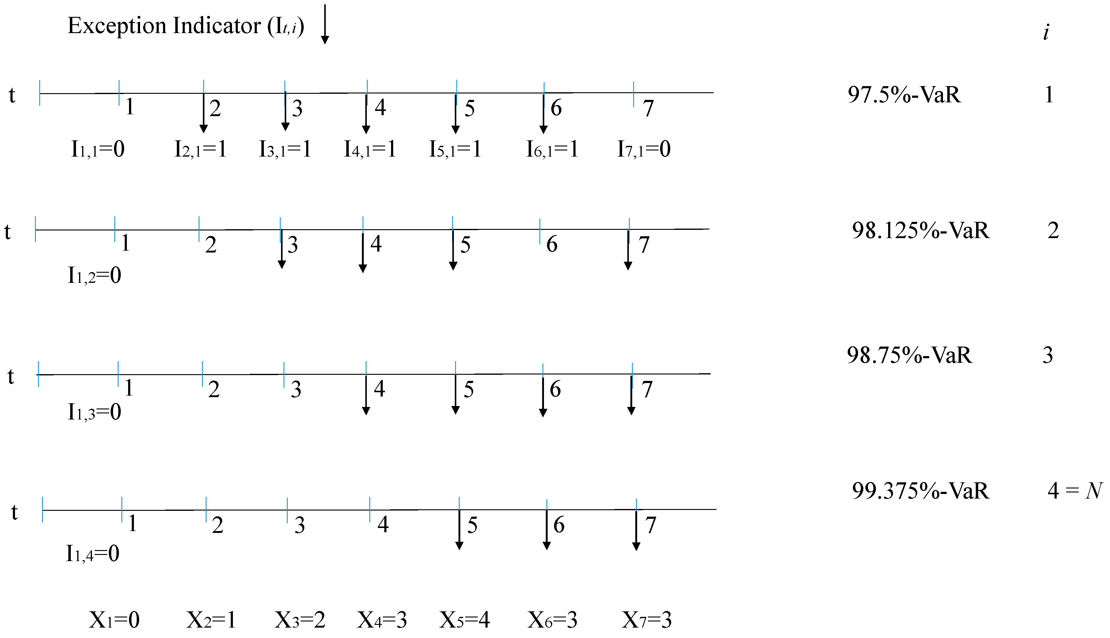
The number of exceptions (violations) are estimated given a certain model (distribution) and for each confidence level. As is typical in the literature, the exception indicator at each time $t$ is defined as a function that takes value 1 if a loss has exceeded the VaR level. That is,

$$I_{t,i}=I_{\left\{L_t>{\mathrm{VaR}}_{{\alpha }_i,t}\right\},}$$

(11)

where ${\alpha }_i$ is as follows:

$${\alpha }_i=\alpha +\frac{i-1}{N}\left(1-\alpha \right),$$

(12)

for $i=1,\dots ,N$, with ${\alpha }_0=0$ and ${\alpha }_{N+1}=1$.

Then, the number of exceptions $X_t$ at each time $t$ is given by

$$X_t={\displaystyle \sum }_{j=1}^N{I}_{t,i}.$$

(13)

As the number of exceptions follows a multinomial distribution, the unconditional coverage property can be written as

$$X_t~\mathrm{MN}\left(1,\left({\alpha }_1-{\alpha }_0,\dots ,{\alpha }_{N+1}-{\alpha }_N\right)\right),$$

(14)

Our interest is a measure that counts the outcomes $\left\{0,1,\dots ,N\right\}$ with probabilities ${\alpha }_1-{\alpha }_0,\dots ,{\alpha }_{N+1}-{\alpha }_N$ that sum to one. The cell counts $O_j$ are then given by

$$O_j={\displaystyle \sum }_{t=1}^n{I}_{\left\{X_t=j\right\}},$$

(15)

where $n$ is the backtesting period and $j=0,1,\dots ,N$. Then, the random vector should follow the multinomial distribution

$$\left(O_0,\dots ,O_N\right)~\mathrm{MN}\left(n,\left({\alpha }_1-{\alpha }_0,\dots ,{\alpha }_{N+1}-{\alpha }_N\right)\right).$$

(16)

The null and alternative hypotheses are given by

H0: θ_i = α_i for i = 1, …, N

H1: θ_i ≠ α_i for at least one i ∈ {1, …, N},

where $0={\theta }_0<{\theta }_1<\dots <{\theta }_{N+1}=1$ is an arbitrary sequence of parameters from a specific model and $\left(O_0,\dots ,O_N\right)~\mathrm{MN}\left(n,\left({\theta }_1-{\theta }_0,\dots ,{\theta }_{N+1}-{\theta }_N\right)\right)$ [2].

Figure 1 illustrates an example for our case (97.5%-ES and $N=4$).

For this case, the number of exceptions $X_t$ for each $t$ is calculated as

$$\begin{gathered} X_{t=1}=I_{1,1}+I_{1,2}+I_{1,3}+I_{1,4}=0, \\ {X}_{t=2}=I_{2,1}+I_{2,2}+I_{2,3}+I_{2,4}=1, \\ ⋮ \\ {X}_{t=7}=I_{7,1}+I_{7,2}+I_{7,3}+I_{7,4}=3. \end{gathered}$$

(17)

The cell counts $O_j$ are given by

$$\begin{gathered} O_0={{\displaystyle \sum }}_{t=1}^n{I}_{\left\{X_t=0\right\}}=1,\mathrm{since}{X}_1=0, \\ {O}_1={{\displaystyle \sum }}_{t=1}^n{I}_{\left\{X_t=1\right\}}=1,\mathrm{since}{X}_2=1, \\ {O}_2={{\displaystyle \sum }}_{t=1}^n{I}_{\left\{X_t=2\right\}}=1,\mathrm{since}{X}_3=2, \\ {O}_3={{\displaystyle \sum }}_{t=1}^n{I}_{\left\{X_t=3\right\}}=3,\mathrm{since}{X}_4,X_6,X_7=3, \\ {O}_4={{\displaystyle \sum }}_{t=1}^n{I}_{\left\{X_t=4\right\}}=1,\mathrm{since}{X}_5=4. \end{gathered}$$

(18)

There are several multinomial tests; the most common is the Pearson chi-squared test, for which the test statistic $S_N$ follows a ${\chi }_N^2$ distribution under the null hypothesis:

$$S_N={\displaystyle \sum }_{j=0}^N\frac{{\left(O_{j+1}-n\left[{\alpha }_{j+1}-{\alpha }_j\right]\right)}^2}{n\left[{\alpha }_{j+1}-{\alpha }_j\right]}~{\chi }_N^2.$$

(19)

The null hypothesis is rejected at a prespecified type I error $\kappa$ when $S_N>{\chi }_N^2\left(1-\kappa \right)$.

Another test is the Nass test, which is an improvement over the previous test when cell probabilities are small [2]. The test statistic is ${\chi }_{\upsilon }^2$ distributed under the null hypothesis:

$$\frac{2\mathrm{E}\left(S_N\right)}{\mathrm{var}\left(S_N\right)}{S}_N~{\chi }_{\upsilon }^2,$$

(20)

where $\mathrm{E}\left(S_N\right)=N$, $\mathrm{var}\left(S_N\right)=2N-\frac{N^2+4N+1}{n}+\frac{1}{n}{{\displaystyle \sum }}_{j=0}^N\frac{1}{\left[{\alpha }_{j+1}-{\alpha }_j\right]}$ and $\upsilon =\frac{2{\left(\mathrm{E}\left(S_N\right)\right)}^2}{\mathrm{var}\left(S_N\right)}$.

The null hypothesis is rejected at a prespecified type I error $\kappa$ when $\frac{2\mathrm{E}\left(S_N\right)}{\mathrm{var}\left(S_N\right)}{S}_N>{\chi }_{\upsilon }^2\left(1-\kappa \right)$.

4. Data

In this section we compare the validation of the risk model of investments that either includes or excludes, shares of companies related to the fossil fuel industry. With this in mind, our data comprise two sets of daily prices detailed as follows. We prepare one of the datasets to consider the companies that are not exposed to unsustainable assets. We refer to these as the sustainable index (SI). It should capture the stock return behaviour of sustainable companies. This first set of data corresponds to FTSE Developed ex Fossil Fuel Total Return Index. This index is a part of the Sustainability and Environmental, Social and Governance (ESG) indexes of FTSE Russell (other indexes with similar characteristics can be found at its website). This index is designed to represent the performance of FTSE All-World Index constituents after the exclusion of companies that have some exposure of revenues and/or reserves to fossil fuels. The second set of data is obtained from the S&P 500 Oil, Gas and Consumable Fuels Index (“Standard and Poor’s 500 Oil, Gas and Consumable Fuels Index is a capitalization-weighted index. The index was developed with a base level of 10 for the 1941-43 base period. The parent index is SPXL3. This is a GICS Level 3 Industries. Standard and Poor’s 500 (Industry) Index is a capitalization-weighted index. The index is designed to measure performance of the broad domestic economy through changes in the aggregate market value of 500 stocks representing all major industries. The index was developed with a base level of 10 for the 1941-43 base periods.” Source: Bloomberg LP). This index includes companies in the energy sector engaged in the exploration, production, refining, marketing, storage and transportation of oil, gas, coal and consumable fuels. It is used as proxy of the whole oil and gas industry and is referred to as the traditional oil and gas index (TI).

Both indexes are capitalization-weighted and enable us to study the risk of investing in broadly diversified portfolios that include or exclude the traditional energy industry. The price data comprise information from 31 July 2006 to 16 November 2018 for a total of 3210 price observations (The selection of the indexes and period is restricted to availability of data from Bloomberg terminal). Moreover, we are interested in the effect of variability of main stranded asset price returns in the variance behaviour of the indexes. To this end, prices of oil, gas and coal have been collected for the same period of SI and TI indexes (The Generic 1^st ‘CL’ Futures (CL1), Generic 1^st ‘NG’ Futures (NG1) and Richards Bay Coal Futures (XO1) are obtained for oil, gas and coal prices, respectively). The abovementioned data are obtained from Bloomberg terminal (Bloomberg Professional Service is an information service that, through subscription, provides economic and financial data at the level of individual securities and the entire market. The workstations with the installed service are traditionally called Bloomberg terminals).

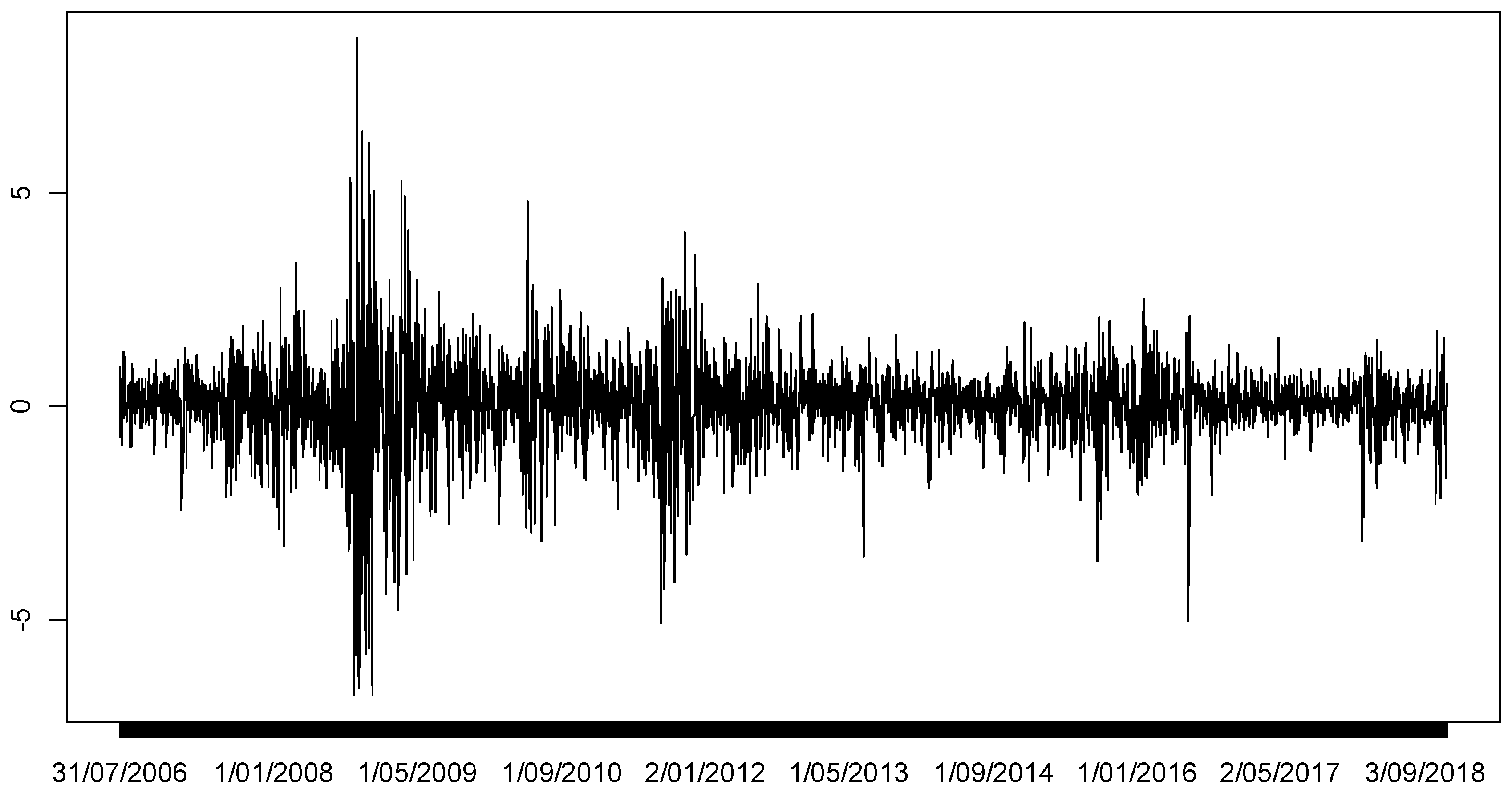
The descriptive statistics (see

Table 1. Descriptive statistics for daily stock returns of the SI (sustainable index) and TI (traditional oil and gas index).

Statistics	SI Returns	TI Returns	Oil Returns	Gas Returns	Coal Returns
Mean	0.024	0.007	−0.008	−0.019	0.016
Median	0.070	0.000	0.000	0.000	0.000
Standard deviation	1.002 (15.85)	1.638 (25.91)	2.324 (36.75)	3.034 (47.97)	1.500 (23.72)
Skewness	−0.489	−0.261	0.134	0.617	0.697
Excess Kurtosis	9.003	13.747	4.968	5.873	44.624
Minimum	−6.785	−16.294	−13.065	−18.054	−20.729
Maximum	8.648	17.208	16.410	26.771	23.841

Figures in percentage. Annual volatility in parentheses. Data range from 31 July 2006 to 16 November 2018 for a total of 3210 price observations.

) show that analysed stock index returns exhibit very well-known stylized facts for financial asset daily returns. The mean and median returns of the TI are close to zero but the SI shows a mean of 0.024% and a median of 0.071%. In terms of daily volatility, the TI shows a standard deviation which is approximately two-thirds larger than the SI. The index returns distributions display fat tails, since excess kurtosis is positive. Moreover, the distributions are negative skewed, which implies more negative extreme values. Figure 2; Figure 3 depict the returns for both indexes. The index returns exhibit similar characteristics and are remarkably affected by the global financial crisis, as exhibited by the high volatility in approximately 2007 and 2008 and the financial problems faced by most companies in oil and gas industry. For the stranded asset returns, gas presents the highest volatility, whereas coal exhibit fatter tails among the three assets. All the analysed asset returns display positive skewed distributions.

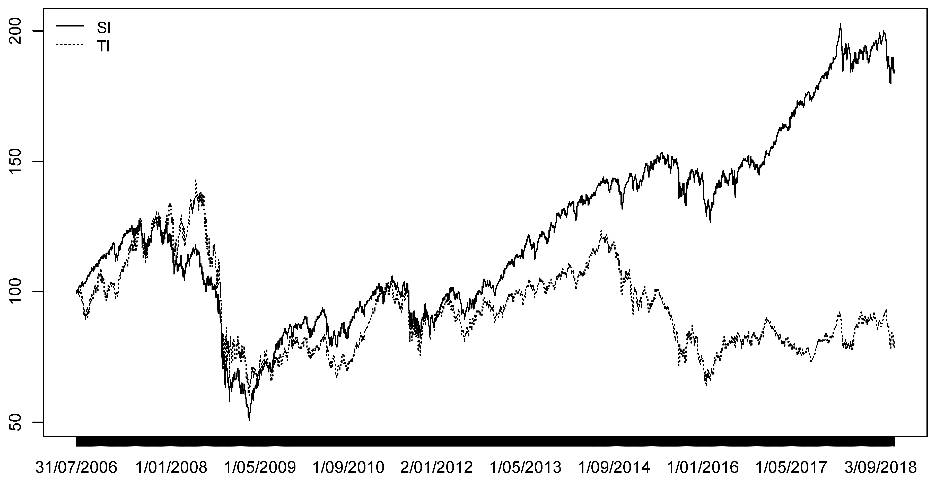
To show the temporal evolution of accumulated returns during the sample period, Figure 4 depicts the value of an initial investment of 100 on each of the indexes on 31 July 2006. During the 2007–2008 global financial crisis, TI investment value is larger than SI investment. However, after such period, particularly since 2012, SI investment has clearly outperformed TI investment. According to the compound annual growth rate (CAGR), the performance of SI investment exceeds that of TI investment during the analysed period. Considering a year of 252 days (12.7 years for 3210 days) and final values (on 16 November 2018) for SI and TI of 184.95 and 80.89 respectively, the CAGR for SI and TI investments are 4.95% and −1.65% respectively.

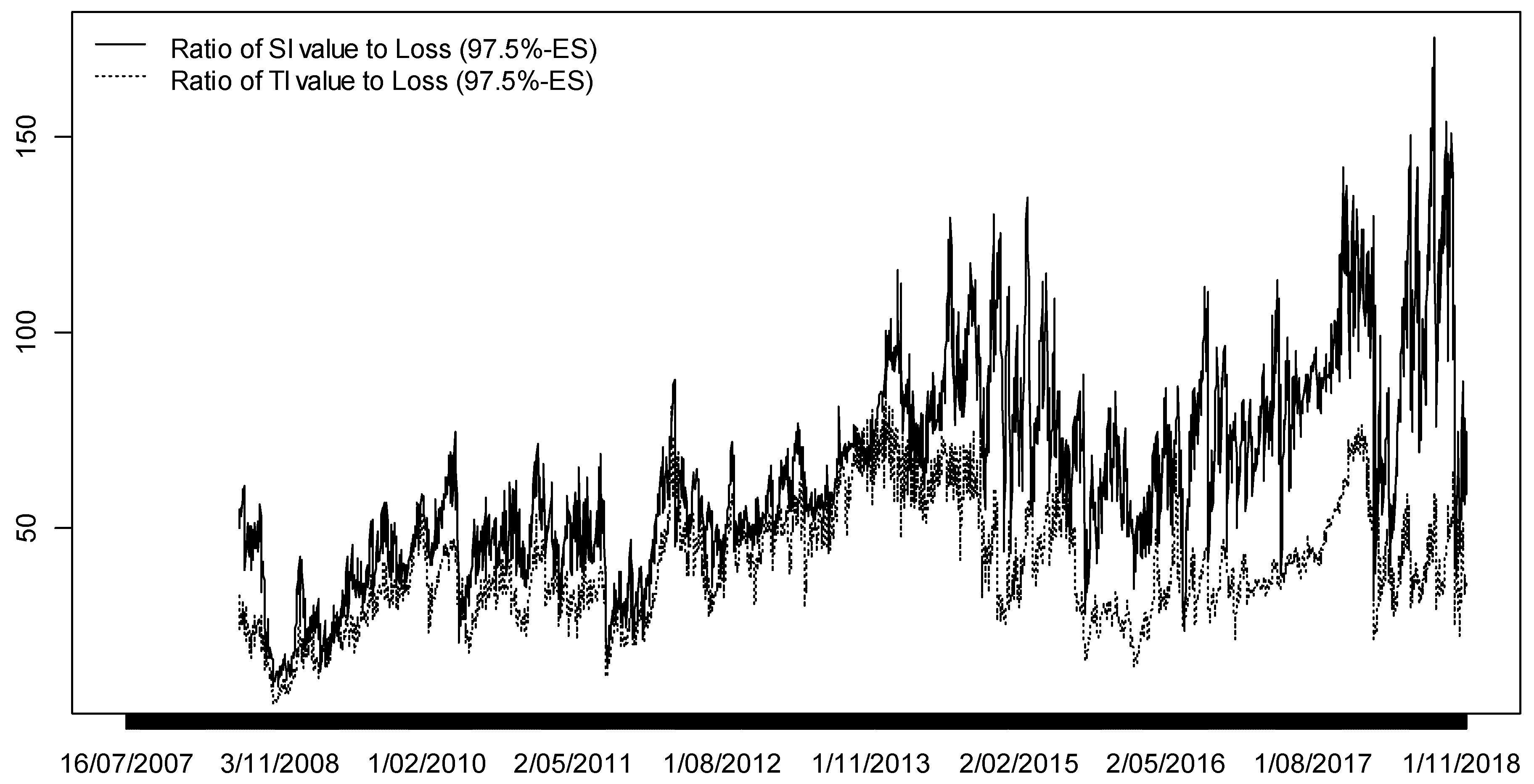
The relationship between risk, as measured by standard deviation and the rate of return of the traditional oil and gas industry index shows a worse performance than that observed for the sustainable asset index. Alternatively, we also analyse the risk-return combination considering ES as the measure of risk. The relation value of SI investment to potential loss outperforms the relation of TI investment to loss during the analysed period, when loss is estimated based on 97.5%-ES (Values of 97.5%-ES estimated for Stable model are employed when external regressors are considered in the GARCH model. Thus, potential loss is calculated as $Los{s}_t=E{S}_t^{97.5}\left(IndexValu{e}_t\right)$). Figure 5 shows the evidence abovementioned.

Beyond other considerations relating to climate change awareness or the risk of further regulation of the fossil fuel industry, that is, from a strictly financial point of view, the global sustainable portfolio excluding fossil fuel industry assets performs better than the portfolio of assets related to the traditional oil and gas industry over the last decade. However, this relatively poor performance on the traditional oil and gas industry assets is not necessarily a bad result. An interesting feature for portfolio managers is the outperformance of this index during the global financial crisis and subsequent period of uncertainty. During these periods, the correlation of these assets with the rest of the market tends to decrease, being very low or even negative. Therefore, these are assets to be included in a portfolio to diversify the overall risk.

5. Statistical Results

This section presents the results of computing VaR and ES from both datasets, SI and TI stock indexes and provides the ES backtesting analysis in comparison with traditional backtesting methods for VaR. The analysis here is primarily quantitative and of a strong statistical nature. The discussion about the implications of these results is delayed until next section.

The backtesting is classified in two cases. One method considers the ARMA-GARCH model with different innovations presented in Section 3.1. to filter the returns of SI and TI indexes, whereas the second method includes the variance of stranded asset (oil, gas and coal) returns as independent variables in the variance equation of GARCH model to filter the returns of the indexes. In-sample estimation results for the whole period are presented in

Table 2. In-Sample results of ARMA-GARCH model fit to the analysed indexes.

Panel A: ARMA-GARCH Estimation
ARMA-GARCH with Gaussian innovations	TI Index	SI Index
${\theta }_0$	0.036 (0.067)	0.058 (0.000)
${\theta }_1$	−0.082 (0.887)	0.023 (0.857)
${\theta }_2$	0.028 (0.961)	0.101 (0.435)
${\beta }_0$	0.023 (0.000)	0.009 (0.000)
${\beta }_1$	0.084 (0.000)	0.105 (0.000)
${\beta }_2$	0.907 (0.000)	0.888 (0.000)
ARMA-GARCH with Student’s t innovations	TI Index	SI Index
${\theta }_0$	0.050 (0.007)	0.071 (0.000)
${\theta }_1$	−0.040 (0.938)	−0.067 (0.656)
${\theta }_2$	−0.013 (0.980)	0.188 (0.206)
${\beta }_0$	0.019 (0.002)	0.006 (0.004)
${\beta }_1$	0.080 (0.000)	0.101 (0.000)
${\beta }_2$	0.913 (0.000)	0.898 (0.000)
$\nu$	6.923 (0.000)	5.414 (0.000)
Panel B: ARMA-GARCH Estimation Considering External Regressors in the variance equation
ARMA-GARCH with Gaussian innovations	TI Index	SI Index
${\theta }_0$	0.035 (0.667)	0.059 (0.000)
${\theta }_1$	−0.081 (0.887)	0.024 (0.855)
${\theta }_2$	0.027 (0.961)	0.102 (0.429)
${\beta }_0$	0.023 (0.003)	0.005 (0.144)
${\beta }_1$	0.083 (0.000)	0.109 (0.000)
${\beta }_2$	0.907 (0.000)	0.881 (0.000)
${\gamma }_1$	0.000 (0.999)	0.000 (0.425)
${\gamma }_2$	0.000 (0.999)	0.000 (0.277)
${\gamma }_3$	0.000 (0.999)	0.000 (0.999)
ARMA-GARCH with Student’s t innovations	TI Index	SI Index
${\theta }_0$	0.050 (0.007)	0.071 (0.000)
${\theta }_1$	−0.040 (0.938)	−0.068 (0.652)
${\theta }_2$	−0.013 (0.980)	0.189 (0.205)
${\beta }_0$	0.019 (0.003)	0.006 (0.093)
${\beta }_1$	0.080 (0.000)	0.103 (0.000)
${\beta }_2$	0.913 (0.000)	0.898 (0.000)
${\gamma }_1$	0.000 (0.999)	0.000 (0.999)
${\gamma }_2$	0.000 (0.999)	0.000 (0.999)
${\gamma }_3$	0.000 (0.999)	0.000 (0.999)
$\nu$	6.923 (0.000)	5.311 (0.000)

P-values in parentheses.

. The results show that the parameters related to oil, gas and coal variances are statistically not significant. In other words, variance of stranded assets does not seem to have explanatory power in the variance of SI and TI returns. In fact, the estimation of ARMA-GARCH parameters when the variances of unsustainable assets are not included in the variance equation does not vary significantly comparing the estimation when the external regressors are taken into account. In what follows, we analyse whether the inclusion of these regressors help improve the backtesting results.

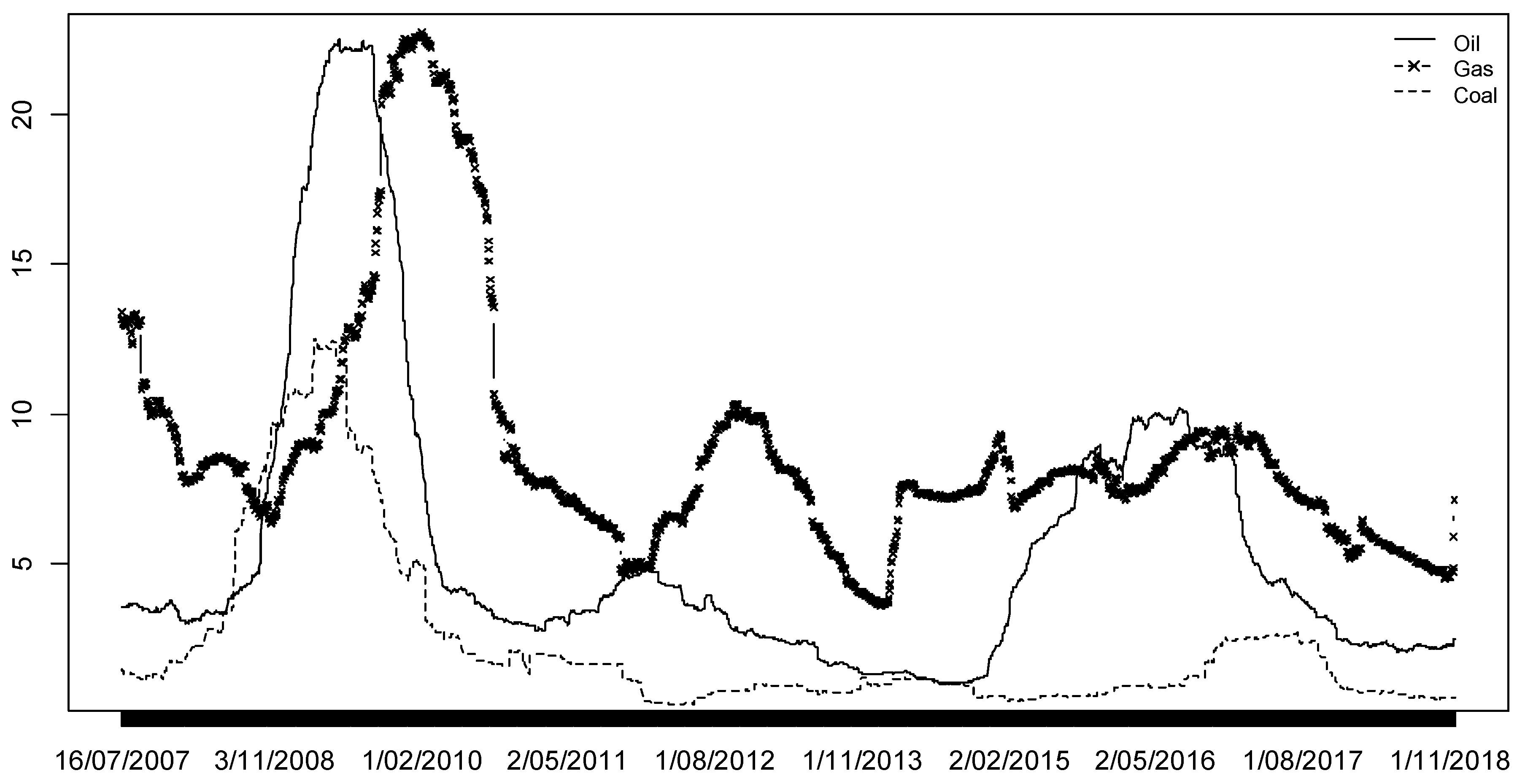
The first 250 returns of oil, gas and coal assets are employed to obtain the first set of values of their respective variances and a rolling window of 250 observations is implemented to estimate the rest of the variances. That is, the initial range of data from 1 August 2006 to 15 July 2007 is employed in order to calculate the variances that act as external regressors. Figure 6 shows the estimated variance of the stranded asset returns. Variability of oil and coal returns were mainly affected by the global financial crisis and high volatility in the gas returns is observed posterior that date. The correlation between log-returns (estimated variance of log-returns) between oil and gas is 0.18 (0.40), for oil and coal is 0.16 (0.78) and for gas and coal is 0.02 (0.32) for the analysed period (The period of 16 July 2007 and 16 November 2018 is considered to estimate the correlations among asset log-returns).

The one-day-ahead VaR and ES are calculated by also implementing a rolling window of 250 observations, then the initial window size is ranged from 16 July 2007 to 29 June 2008. The backtesting period for both analysed indexes (SI and TI) ranged from 30 June 2008 to 16 November 2018 and its length period is 2709 days. Thus, the expected number of exceptions is 27.09 (approximated to 27 in

Table 3. Comparison of 99%-VaR and 97.5%-ES (implicit) backtesting for the Sustainable Index (SI) and the Traditional Oil and Gas Industry (TI).

Model	99% VaR		97.5% ES
	EE	Violations	${\mathit{O}}_0$	${\mathit{O}}_1$	${\mathit{O}}_2$	${\mathit{O}}_3$	${\mathit{O}}_4$	Pearson	Nass
Panel a) Sustainable Index (SI):
Normal	27	33 (0.270)	2644	13	17	10	25	7.60	7.39
Student’s-t	27	11 (0.000)	2658	9	21	10	11	9.71	9.45
Stable	27	32 (0.357)	2631	21	19	16	12	2.84	2.76
GPD-POT	27	15 (0.011)	2654	17	20	10	8	8.17	7.94
Panel b) Traditional Oil & Gas Industry (TI):
Normal	27	32 (0.357)	2648	9	17	14	21	5.22	5.07
Student’s-t	27	14 (0.005)	2657	14	8	16	14	5.87	5.71
Stable	27	32 (0.357)	2638	9	21	17	24	7.65	7.44
GPD-POT	27	20 (0.151)	2660	13	13	9	14	6.18	6.01

EE stands for Expected Exceptions. The critical value for the Pearson test is 9.49 and that for the Nass test is 9.31. The P-value for the binomial test in parenthesis. $O_j$ ($j=0,1,2,3,4$) counts the times the number of exceptions ($X_t$) are equal to $j$ for each time t and for all VaR levels. Backtesting periods include 2709 days for the SI and the TI portfolios. Figures in red colour indicates bad performance of the model.

;

Table 4. Comparison of 99%-VaR and 97.5%-ES (implicit) backtesting for the Sustainable Index (SI) and the Traditional Oil and Gas Industry (TI). Considering external regressors in the variance equation of GARCH model.

Model	99% VaR		97.5% ES
	EE	Violations	${\mathit{O}}_0$	${\mathit{O}}_1$	${\mathit{O}}_2$	${\mathit{O}}_3$	${\mathit{O}}_4$	Pearson	Nass
Panel a) Sustainable Index (SI):
Normal	27	33 (0.270)	2641	15	16	13	24	4.13	4.02
Student’s-t	27	17 (0.036)	2655	12	21	10	11	7.40	7.20
Stable	27	32 (0.357)	2633	19	17	17	23	2.45	2.39
GPD-POT	27	20 (0.151)	2649	15	21	11	13	4.21	4.10
Panel b) Traditional Oil & Gas Industry (TI):
Normal	27	35 (0.144)	2643	11	18	14	23	4.83	4.70
Student’s-t	27	23 (0.417)	2650	18	10	18	13	3.91	3.81
Stable	27	34 (0.199)	2630	15	21	18	25	5.16	5.02
GPD-POT	27	25 (0.683)	2655	14	10	11	19	5.75	5.59

EE stands for Expected Exceptions. The critical value for the Pearson test is 9.49 and that for the Nass test is 9.31. The P-value for the binomial test in parenthesis. $O_j$ ($j=0,1,2,3,4$) counts the times the number of exceptions ($X_t$) are equal to $j$ for each time t and for all VaR levels. Backtesting periods include 2709 days for the SI and the TI portfolios. Figures in red colour indicates bad performance of the model.

) for both indexes when calculating 99%-VaR.

Table 3 presents the results of testing VaR and ES for both the SI and the TI when the variance of unsustainable assets is not considered in the GARCH model. We compute the well-known binomial tests for VaR at 99% and the two new multinomial tests, that is, the Pearson and Nass statistics, proposed by [2], for 97.5%-ES backtesting. In the case of the sustainable index, the binomial test for VaR rejects the Student’s t and GPD models, since both models overpredict risk for the index returns. In most applications of market risk quantification, results of EVT techniques based on GPD model are favourable. However, in this case, the binomial test for 99%-VaR rejects the good performance of this model. A plausible reason is that the amount of observations (in the tail of the empirical distribution) employed to fit the GPD, which is 25 in each step of the rolling window. It is very well-known that parameter estimation depends on the threshold selection, which is still an open question in EVT and this drawback is discussed for instance in Reference [54]. Backtesting ES of the SI, the results of Pearson and Nass tests do not reject the good performance of normal, Stable and GPD models but Student’s t model does not perform satisfactorily, which is consistent with backtesting of VaR results for the same index (Table 3, Panel a).

In the case of the traditional oil and gas industry index returns, only the Student’s t model does not perform well according to the binomial test for 99%-VaR (Table 3, Panel b), whereas all the models perform well for 97.5%-ES backtesting, according to Pearson and Nass statistics.

Table 4 replicates analysis of Table 3 but the new analysis considers the external regressors in the equation of variance (Equation (1)). Although the binomial test for 99%-VaR still rejects the good performance of the Student’s t model, all other models now exhibit a reasonable performance for VaR and ES tests. This is an important result, since there is evidence that employing external regressors (variance of stranded asset returns) help improve risk model validations for the analysed data in our paper.

We also conduct the simple backtest of ES, commonly used in the literature, as a robustness check of the new multinomial test previously applied to validate ES.

Table 5. Exceptions obtained for each VaR level for the Sustainable Index (SI) and the Traditional Oil and Gas Index (TI).

Model	97.5%VaR	98.125%VaR	98.75%VaR	99.375%VaR
Panel a) Sustainable Index (SI):
	[52;84] EE = 68	[37;65] EE = 51	[23;45] EE = 34	[9;25] EE = 17
Normal	65	52	35	25
Student’s-t	51	42	21	11
Stable	78	57	38	22
GPD-POT	55	38	18	8
Panel b) Traditional Oil & Gas Industry (TI):
	[52;84] EE = 68	[37;65] EE = 51	[23;45] EE = 34	[9;25] EE = 17
Normal	61	52	35	21
Student’s-t	52	38	30	14
Stable	71	62	41	24
GPD-POT	49	36	23	14

EE stands for Expected Exceptions. 95% confidence interval in brackets for each expected number of exceptions. Backtesting periods include 2709 days for the SI and the TI portfolios. Figures in red colour indicates bad performance of the model.

shows the results of independent individual binomial backtests of VaR for four confidence levels equal to and higher than that used in the 97.5% ES estimate. This analysis is performed for both indexes without considering external regressors in variance equation. This methodology based on independent testing for different confidence levels provides results similar to those obtained in the multinomial test for three loss distributions. However, it indicates that the GPD model overpredicts risk when VaR is calculated at 98.75% and 99.375% (97.5% and 98.125%) confidence levels for SI (TI) index return as can be seen in Table 5, Panel a (Panel b). Anyway, the results for the Pearson and Nass tests for 97.5%-ES displayed in Table 3, which rejects the Student’s t model and shows that the normal and Stable models perform well for both indexes, are also confirmed by the individual binomial tests.

Table 6. Exceptions obtained for each VaR level for the Sustainable Index (SI) and the Traditional Oil and Gas Index (TI). Considering external regressors in the variance equation of GARCH model.

Model	97.5%VaR	98.125%VaR	98.75%VaR	99.375%VaR
Panel a) Sustainable Index (SI):
	[52;84] EE = 68	[37;65] EE = 51	[23;45] EE = 34	[9;25] EE = 17
Normal	68	53	37	24
Student’s-t	54	42	21	11
Stable	76	57	40	23
GPD-POT	60	45	24	13
Panel b) Traditional Oil & Gas Industry (TI):
	[52;84] EE = 68	[37;65] EE = 51	[23;45] EE = 34	[9;25] EE = 17
Normal	66	55	37	23
Student’s-t	59	41	31	13
Stable	79	64	43	25
GPD-POT	54	40	30	19

EE stands for Expected Exceptions. 95% confidence interval in brackets for each expected number of exceptions. Backtesting periods include 2709 days for the SI and the TI portfolios. Figures in red colour indicates bad performance of the model.

presents same results as Table 5 considering variance of unsustainable asset returns as independent variables in the variance equation of the GARCH model. Only Student’s t model is rejected when 98.75%-VaR is calculated for SI index returns. Once again, the risk model performance is enhanced when the variances of stranded asset returns are included as regressors in the variance equation to assess VaR at different confidence levels.

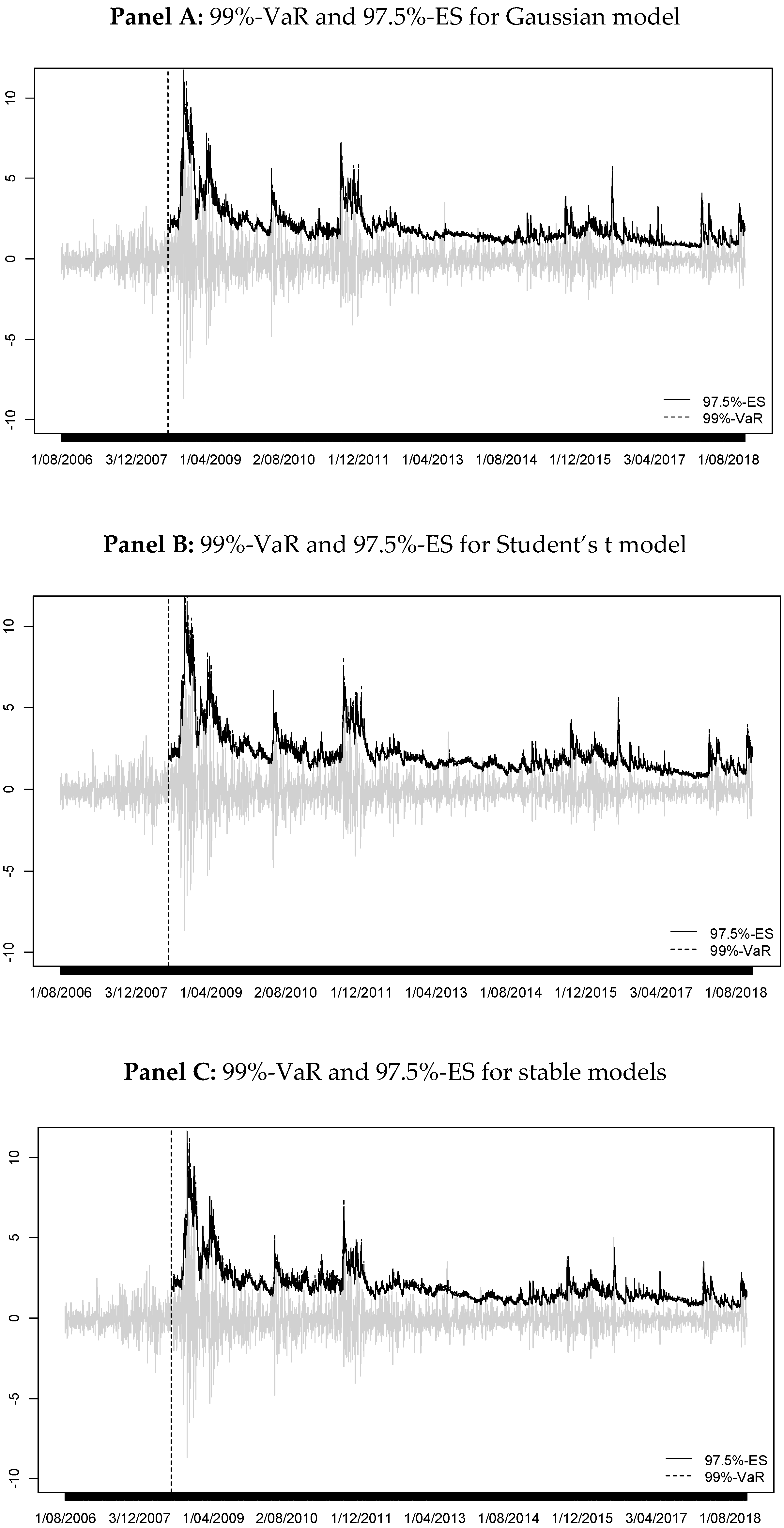
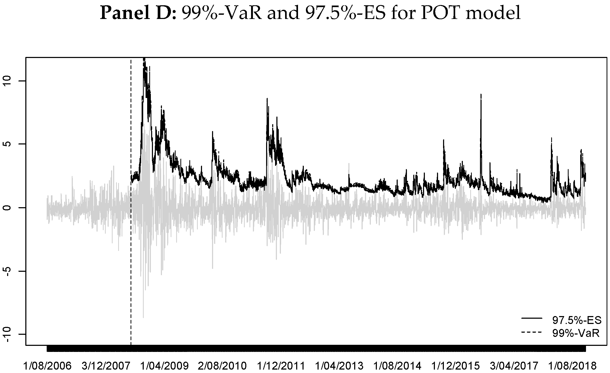
Finally, Figure 7 shows the comparison of 99%-VaR and 97.5%-ES (with external regressors in the variance equation) for each analysed model applied to SI returns (Similar results are obtained for Portfolio TI returns and are available upon request and for both indexes when external regressors are not included in the variance equation in GARCH model). As expected, 99%-VaR is similar to 97.5%-ES for the Gaussian case; however, it is noted that 97.5%-ES is higher than 99%-VaR for stable and GPD cases. This result corroborates one of the arguments used by the Basel Committee to defend the use of ES to calculate the market risk of a financial institution.

6. Discussion, Conclusions and Future Work

Energy assets have higher volatilities than other types of stocks and are affected by a trend towards divestment caused by greater global awareness of the environmental and financial impact of climate change. Nevertheless, portfolio managers and institutional investors in general have big interest on energy assets due to their importance for diversification purposes and, in these days, the predominant role of fuel-based industries in energy portfolios is clearly being replaced by sustainable alternatives. This change in paradigm implies new challenges to policy makers and managers and they have to count on trustable risk measures and accompanying backtesting procedures, that must be in agreement with the recently proposed guidelines about financial investments proposed by the regulators. To address this issue, as described in Section 4, we have constructed and analysed two very different indexes: one formed by companies in the traditional energy industry (TI) and a second one of a sustainable nature (SI). We have collected data from these portfolios during an extensive period of time. For these datasets, in Section 5 we have performed a large experiment where we have utilized several proposed probabilistic models from which we have computed a number of risk measures that we have tested using two different backtesting methods.

Our results show that, in general, sustainable investments statistically behave similarly to traditional assets but in terms of returns these are outperforming traditional ones in the last decade. Nevertheless and quite interestingly, the situation is the reverse in periods of crisis when additionally, returns of both portfolios show low or even negative correlation. These findings suggest that investments on sustainable industries may assume the role of traditional fuel-based energy industries in designing well diversified portfolios. Also, our results point out that a combination of both could be interesting trying to anticipate structural changes on investments during turmoil periods. All this would imply that, by incorporating traditional energy industry stocks into portfolios of sustainable companies, the financing of these latter companies can be improved and, therefore, they can enjoy better financing of their sustainable development projects. In summary, our findings on proper risk measurement are potentially beneficial for sustainable development. Investors and portfolio managers may perceive investment in sustainable companies as more desirable if they can diversify or reduce the inherent market risk.

From a modeler perspective and in terms of methods to implement VaR but especially ES, our experiment provides several interesting conclusions and recommendations. In particular results of VaR and (implicit) ES backtesting seem to indicate that external regressors should be considered in the GARCH equation. In particular, we have found evidence that the variances of unsustainable assets (i.e., the exogenous regressors) help to improve the variance estimation of the TI and SI returns and therefore the backtesting performance. These results are in line with [61,62,63,64]. Gaussian and Stable distributions perform comparatively better in all situations and hence these are the statistical models we recommend for constructing risk measure methodologies in applications with substantial energy-based investments.

Obviously and not less important particularly to policy-makers is the question of ES backtesting. To the best of our knowledge, our paper is the first time that multinomial tests have been applied to SI and TI assets and that exogenous variables are included to improve the performance of the forecast volatility model. The backtesting procedure we implement is based on multinomial tests for different VaR levels rather than performing a binomial test for each VaR level, since ES can be approximated in terms of multiple VaRs [59]. We obtain evidence that the multinomial test is an adequate and simple method to validate ES models as presented in this paper. This simple approach leads to an implicit manner for ES backtesting and it is suggested for regulatory purposes.

Future research can be conducted to compare other ES tests such as those proposed by [58]. A possible limitation of our work is that ES is approximated by just four terms of VaR levels. Though more VaR figures employed in the ES approximation can provide a more accurate ES measure, [2] show that employing four VaR levels produce good results regarding size and power of the multinomial test and it is more powerful than a single binomial test. Then future research can be focused on employing eight VaR levels, which also performs well according to [2], for the multinomial test. In addition, other ES tests proposed in the future can be compared with the multinomial test employed in this paper. Another limitation is the window size (250 days), suggested by Basel Committee, may be not enough when calculating VaR at high probability levels and this is also noted by [2]. Parameter estimation of GARCH models can be biased in small samples and a window of 500 days is recommended when this type of models is employed [65]. Moreover, parameter estimates of generalized Pareto distribution exhibits high variance in small samples when peaks-over-threshold method is utilized and risk measures may be wrongly assessed. This was evidenced in our empirical application and several window sizes can be tested in future research. This paper analysed the risk quantification for individual assets. Further research may be focused on ES testing of traditional energy and sustainable investment portfolios, where multivariate models (such as DCC, BEKK, copula, among others) can be employed to analyse the correlation and dependence structure of different assets. Finally, a main concern is to quantify the economic loss caused by climate change. A first attempt of climate VaR estimation is developed by the [39]. Future work could be the estimation of losses once those losses have exceeded climate VaR by employing some of the techniques in our paper.

References

- Adams, C.; Wilson, J.; Vandevelde, M. Moody’s Puts 175 Energy and Mining Companies on Downgrade Watch. Financial Times. 2016. Available online: https://www.ft.com/content/bfa6f25a-c0ea-11e5-9fdb-87b8d15baec2 (accessed on 15 October 2018).
- Kratz, M.; Lock, Y.; McNeil, A.J. Multinomial VaR backtests: A simple implicit approach to backtesting expected shortfall. J. Bank. Financ. 2018, 88, 393–407. [Google Scholar] [CrossRef] [Green Version]
- Chen, J.M. On Exactitude in Financial Regulation: Value-at-Risk, Expected Shortfall, and Expectiles. Risks 2018, 6, 61. [Google Scholar] [CrossRef]
- Fischer, M.; Moser, T.; Pfeuffer, M. A Discussion on Recent Risk Measures with Application to Credit Risk: Calculating Risk Contributions and Identifying Risk Concentrations. Risks 2018, 6, 142. [Google Scholar] [CrossRef]
- Christoffersen, P. Evaluating interval forecasts. Int. Econ. Rev. 1998, 39, 841–862. [Google Scholar] [CrossRef]
- Cabedo, J.D.; Moya, I. Estimating oil price ‘value at risk’ using the historical simulation approach. Energy Econ. 2003, 25, 239–253. [Google Scholar] [CrossRef]
- Ewing, B.T.; Malik, F. Estimating volatility persistence in oil prices under structural breaks. Financ. Rev. 2010, 45, 1011–1023. [Google Scholar] [CrossRef]
- Feng, Z.H.; Wei, Y.M.; Wang, K. Estimating risk for the carbon market via extreme value theory: An empirical analysis of the EU ETS. Appl. Energy 2012, 99, 97–108. [Google Scholar] [CrossRef]
- Costello, A.; Asem, E.; Gardner, E. Comparison of historically simulated VaR: Evidence from oil prices. Energy Econ. 2008, 30, 2154–2166. [Google Scholar] [CrossRef]
- Fan, Y.; Zhang, Y.-J.; Tsai, H.-T.; Wei, Y.-M. Estimating ‘Value at Risk’ of crude oil price and its spillover effect using the GED-GARCH approach. Energy Econ. 2008, 30, 3156–3171. [Google Scholar] [CrossRef]
- Hung, J.C.; Lee, M.C.; Liu, H.C. Estimation of value-at-risk for energy commodities via fat-tailed GARCH models. Energy Econ. 2008, 30, 1173–1191. [Google Scholar] [CrossRef]
- Marimoutou, V.; Raggad, B.; Trabelsi, A. Extreme Value Theory and Value at Risk: Application to oil market. Energy Econ. 2009, 31, 519–530. [Google Scholar] [CrossRef] [Green Version]
- Youssef, M.; Belkacem, L.; Mokni, K. Value-at-Risk estimation of energy commodities: A long-memory GARCH–EVT approach. Energy Econ. 2015, 51, 99–110. [Google Scholar] [CrossRef]
- Bunn, D.; Andresen, A.; Chen, D.; Westgaard, S. Analysis and Forecasting of Electricity Price Risks with Quantile Factor Models. Energy J. 2016, 37, 101–122. [Google Scholar] [CrossRef]
- Lux, T.; Segnon, M.; Gupta, R. Forecasting crude oil price volatility and value-at-risk: Evidence from historical and recent data. Energy Econ. 2016, 56, 117–133. [Google Scholar] [CrossRef] [Green Version]
- Wang, Y.; Liu, L.; Ma, F.; Wu, C. What the investors need to know about forecasting oil futures return volatility. Energy Econ. 2016, 57, 128–139. [Google Scholar] [CrossRef]
- Lyu, Y.; Wang, P.; Wei, Y.; Ke, R. Forecasting the VaR of crude oil market: Do alternative distributions help? Energy Econ. 2017, 66, 523–534. [Google Scholar] [CrossRef]
- Ewing, B.T.; Malik, F.; Anjum, H. Forecasting value-at-risk in oil prices in the presence of volatility shifts. Rev. Financ. Econ. 2018. [Google Scholar] [CrossRef]
- Nomikos, N.; Pouliasis, P. Forecasting petroleum futures markets volatility: The role of regimes and market conditions. Energy Econ. 2011, 33, 321–337. [Google Scholar] [CrossRef]
- Segnon, M.; Lux, T.; Gupta, R. Modeling and forecasting the volatility of carbon dioxide emission allowance prices: A review and comparison of modern volatility models. Renew. Sust. Energ. Rev. 2017, 69, 692–704. [Google Scholar] [CrossRef] [Green Version]
- Huang, D.; Yu, B.; Fabozzi, F.J.; Fukushima, M. CAViaR-based forecast for oil price risk. Energy Econ. 2008, 31, 511–518. [Google Scholar] [CrossRef]
- Chiu, Y.-C.; Chuang, I.-Y.; Lai, J.-Y. The performance of composite forecast models of value-at-risk in the energy market. Energy Econ. 2010, 32, 423–431. [Google Scholar] [CrossRef]
- He, K.; Li, K.K.; Yen, J. Value-at-risk estimation of crude oil price using MCA based transient risk modeling approach. Energy Econ. 2011, 33, 903–911. [Google Scholar] [CrossRef]
- Herrera, R. Energy risk management through self-exciting marked point process. Energy Econ. 2013, 38, 64–76. [Google Scholar] [CrossRef]
- Aloui, R.; Aïssa, M.S.B.; Hammoudeh, S.; Nguyen, D.K. Dependence and extreme dependence of crude oil and natural gas prices with applications to risk management. Energy Econ. 2014, 42, 332–342. [Google Scholar] [CrossRef]
- Jäschke, S. Estimation of risk measures in energy portfolios using modern copula techniques. Comput. Stat. Data Anal. 2014, 76, 359–376. [Google Scholar] [CrossRef] [Green Version]
- Zolotko, M.; Okhrin, O. Modelling the general dependence between commodity forward curves. Energy Econ. 2014, 43, 284–296. [Google Scholar] [CrossRef] [Green Version]
- Ghorbel, A.; Trabelsi, A. Energy portfolio risk management using time-varying extreme value copula methods. Econ. Model. 2014, 38, 470–485. [Google Scholar] [CrossRef]
- Lu, X.F.; Lai, K.K.; Liang, L. Portfolio value-at-risk estimation in energy futures markets with time-varying copula-GARCH model. Ann. Oper. Res. 2014, 219, 333–357. [Google Scholar] [CrossRef]
- González-Pedraz, C.; Moreno, M.; Peña, J.I. Tail risk in energy portfolios. Energy Econ. 2014, 46, 422–434. [Google Scholar] [CrossRef]
- Artzner, P.; Delbaen, F.; Eber, J.-M.; Heath, D. Coherent measures of risk. Math. Finance 1999, 9, 203–228. [Google Scholar] [CrossRef]
- Barone Adesi, G. VaR and CVaR Implied in Option Prices. J. Risk Financ. Manag. 2016, 9, 2. [Google Scholar] [CrossRef]
- Dobrev, D.; Nesmith, T.D.; Oh, D.H. Accurate Evaluation of Expected Shortfall for Linear Portfolios with Elliptically Distributed Risk Factors. J. Risk Financ. Manag. 2017, 10, 5. [Google Scholar] [CrossRef]
- Fuertes, A.-M.; Olmo, J. On Setting Day-Ahead Equity Trading Risk Limits: VaR Prediction at Market Close or Open? J. Risk Financ. Manag. 2016, 9, 10. [Google Scholar] [CrossRef]
- Allen, D.E.; McAleer, M.; Powell, R.J.; Singh, A.K. Down-Side Risk Metrics as Portfolio Diversification Strategies across the Global Financial Crisis. J. Risk Financ. Manag. 2016, 9, 6. [Google Scholar] [CrossRef]
- Yu, X.; Sun, H. Optimal Hedging with Options and Futures against Price Risk and Background Risk. Math. Comput. Appl. 2017, 22, 5. [Google Scholar] [CrossRef]
- Weber, S. Distribution-invariant risk measures, information, and dynamic consistency. Math. Finance 2006, 16, 419–441. [Google Scholar] [CrossRef]
- Gneiting, T. Making and evaluating point forecasts. J. Am. Stat. Assoc. 2011, 106, 746–762. [Google Scholar] [CrossRef]
- The Economist Intelligence Unit. The Cost of Inaction: Recognising the Value at Risk from Climate Change; The Economist Intelligence Unit Limited: London, UK; New York, NY, USA; Hong Kong, China; Geneva, Switzerland, 2015. [Google Scholar]
- Bruno, S.V.B.; Sagastizábal, C. Optimization of real asset portfolio using a coherent risk measure: Application to oil and energy industries. Optim. Eng. 2010, 12, 257–275. [Google Scholar] [CrossRef]
- Tekiner-Mogulkoc, H.; Coit, D.W.; Felder, F.A. Mean-risk stochastic electricity generation expansion planning problems with demand uncertainties considering conditional value-at-risk and maximum regret as risk measures. Electr. Power Energy Syst. 2015, 73, 309–317. [Google Scholar] [CrossRef]
- Hemmati, R.; Saboori, H.; Saboori, S. Stochastic risk-averse coordinated scheduling of grid integrated energy storage units in transmission constrained wind-thermal systems within a conditional value-at-risk framework. Energy 2016, 113, 762–775. [Google Scholar] [CrossRef]
- Lu, Z.G.; Qi, J.T.; Wen, B.; Li, X.P. A dynamic model for generation expansion planning based on conditional value-at-risk theory under low-carbon economy. Electr. Power Syst. Res. 2016, 141, 363–371. [Google Scholar] [CrossRef]
- Roustai, M.; Rayati, M.; Sheikhi, A.; Ranjbar, A. A scenario-based optimization of Smart Energy Hub operation in a stochastic environment using conditional-value-at-risk. Sustain. Cities Soc. 2018, 39, 309–316. [Google Scholar] [CrossRef]
- Alizadeh, A.H.; Nomikos, N.K.; Pouliasis, P.K. A Markov regime switching approach for hedging energy commodities. J. Bank. Financ. 2008, 32, 1970–1983. [Google Scholar] [CrossRef]
- Conlon, T.; Cotter, J. Downside risk and the energy hedger’s horizon. Energy Econ. 2013, 36, 371–379. [Google Scholar] [CrossRef]
- Chai, S.; Zhou, P. The Minimum-CVaR strategy with semi-parametric estimation in carbon market hedging problems. Energy Econ. 2018, 76, 64–75. [Google Scholar] [CrossRef]
- McNeil, A.J.; Frey, R. Estimation of tail-related risk measures for heteroscedastic financial time series: An extreme value approach. J. Empir. Finance 2000, 7, 271–300. [Google Scholar] [CrossRef]
- McNeil, A.J.; Frey, R.; Embrechts, P. Quantitative Risk Management: Concepts, Techniques and Tools; Princeton University Press: Princeton, NJ, USA, 2005. [Google Scholar]
- Ghalanos, A. Introduction to the Rugarch Package, (Version 1.3-1). 2015. Available online: https://goo.gl/1nsPNP (accessed on 15 September 2018).
- Nolan, J.P. Maximum likelihood estimation and diagnostics for stable distributions. In Lévy Processes; Barndorff-Nielsen, E., Mikosch, T., Resnick, S., Eds.; Brikhäuser: Boston, MA, USA, 2001. [Google Scholar]
- Chavez-Demoulin, V. Two Problems in Environmental Statistics: Capture-Recapture Analysis and Smooth Extremal Models. Ph.D. Thesis, Department of Mathematics, Swiss Federal Institute of Technology, Lausanne, Switzerland, 1999. [Google Scholar]
- Araújo Santos, P.; Fraga Alves, M.I. Forecasting Value-at-Risk with a duration-based POT method. Math. Comput. Simul. 2013, 94, 295–309. [Google Scholar] [CrossRef]
- Díaz, A.; García-Donato, G.; Mora-Valencia, A. Risk quantification in turmoil markets. Risk Manag. 2017, 19, 202–224. [Google Scholar] [CrossRef]
- Pfaff, B.; McNeil, A.; Pfaff, M.B. Package ‘evir’: Extreme Values in R. R package version 1.7-4. 2018. Available online: https://CRAN.R-project.org/package=evir (accessed on 15 September 2018).
- Fissler, T.; Ziegel, J.F. Higher order elicitability and Osband’s principle. Ann. Stat. 2016, 44, 1680–1707. [Google Scholar] [CrossRef] [Green Version]
- Del Brio, E.B.; Mora-Valencia, A.; Perote, J. Risk quantification for commodity ETFs: Backtesting value-at-risk and expected shortfall. Int. Rev. Financ. Anal. 2017. [Google Scholar] [CrossRef]
- Acerbi, C.; Székely, B. Back-testing expected shortfall. Risk Mag. 2014, 27, 76–81. [Google Scholar]
- Emmer, S.; Kratz, M.; Tasche, D. What is the best risk measure in practice? J. Risk 2015, 18, 31–60. [Google Scholar] [CrossRef]
- Acerbi, C.; Tasche, D. On the coherence of expected shortfall. J. Bank. Financ. 2002, 26, 1487–1503. [Google Scholar] [CrossRef] [Green Version]
- Khindanova, I.; Rachev, S.; Schwartz, E. Stable modeling of value at risk. Math. Comput. Model. 2001, 34, 1223–1259. [Google Scholar] [CrossRef]
- Marinelli, C.; D’Addona, S.; Rachev, S. A comparison of some univariate models for Value-at-Risk and expected shortfall. Int. J. Theor. Appl. Finance 2007, 10, 1043–1075. [Google Scholar] [CrossRef]
- Güner, B.; Rachev, S.; Edelman, D.; Fabozzi, F.J. Bayesian Inference for Hedge Funds with Stable Distribution of Returns. In En Rethinking Risk Measurement and Reporting: Volume II; Böcker, K., Ed.; Risk Books: London, UK, 2010; pp. 95–136. [Google Scholar]
- Rachev, S.; Racheva-Iotova, B.; Stoyanov, S. Capturing fat tails. Risk Mag. 2010, 23, 72–77. [Google Scholar]
- Hwang, S.; Valls Pereira, P.L. Small sample properties of GARCH estimates and persistence. Eur. J. Finance 2006, 12, 473–494. [Google Scholar] [CrossRef]
Figure 1.
Graphical representation for multiple VaR backtesting.
Figure 2.
Sustainable Index (SI) returns.
Figure 3.
Traditional oil and gas industry Index (TI) returns.
Figure 4.
Value of an initial investment of 100 on each index.
Figure 5.
Ratio of value index to potential loss.
Figure 6.
Variance of Oil, Gas and Coal price returns.
Figure 7.
Comparison of 99%-VaR and 97.5%-ES for each model for SI negative log-returns.