Mapping and Characterizing Spatiotemporal Dynamics of Impervious Surfaces Using Landsat Images: A Case Study of Xuzhou, East China from 1995 to 2018

Abstract

As an effective indicator of urbanization, impervious surfaces play a significant role in urban planning and ecological protection. It is, therefore, important to characterize impervious surfaces in urban geographical studies. As a key city in East China, Xuzhou has experienced rapid urbanization in recent decades and is now becoming an environmentally friendly city. To better understand the spatiotemporal heterogeneity of Xuzhou’s urban development, we extracted its impervious surfaces from Landsat images of 1995, 2003, 2010, and 2018 by a linear spectral mixture analysis. Then, a range of complementary methods including landscape indices, profile lines, median centers, standard deviational ellipses, and spatial autocorrelation were adopted to analyze the landscape pattern and expansion of impervious surfaces on both city and district scales. Results show that (1) there was a constant impervious surface expansion, originating in downtown Xuzhou; (2) promoting ecological protection in urban areas fragmented impervious surfaces with increasing heterogeneity and diversity overall; and (3) expansion directions and rates of impervious surfaces varied with district and town, and the central urban area expanded towards east and southeast, which could be related to their own resources and governmental policies. Findings from this study provide useful insights into urban planning of this economically prospective region.

1. Introduction

As population continues to increase, urbanization has become a universal and important phenomenon in the world. Urban expansion is one of the basic characteristics of urbanization, impacting urban ecosystem and changing urban land use structure and landscape pattern [1]. As such, appropriate methods are needed to accurately reflect the spatiotemporal variation of urban expansion, to understand the dynamics of regional urbanization.

A number of methods for mapping urban expansion exist, such as lognormal regression model [2], self-organizing map approach [3], landscape index [4,5], and (un-)supervised classification [6,7,8,9,10,11]. As the major component of land cover in urban areas, impervious surface (IS), i.e., artificial materials which water cannot penetrate, provides a key piece information on urban ecosystems and urban growth [12]; therefore, is mostly used as a proxy for urban expansion [6,13,14]. Commonly used methods for mapping impervious surfaces include spectral indices [15,16], supervised classification [17] or a linear spectral mixture analysis (LSMA) [13,14,18,19,20], but the latter is preferable to the former as it is more physically meaningful.

LSMA models an image pixel as a linear mixture of materials present in an image [19]. It has been widely used including model parameter estimation [21,22], land use classification [23,24], estimation of agricultural yield [25], estimation of forest carbon density [26], identification and analysis of specific land type, such as coffee crops [27], lava flows [28], and impervious surfaces [29,30]. When the LSMA is used for mapping impervious surfaces to characterize urban expansion, it is often combined with the vegetation–impervious surface–soil (VIS) model [31,32], which considers urban surfaces as a combination of vegetation, soil, high-, and low-albedo impervious surfaces with water masked out. Examples include the study by Kuang et al. (2014) [13] that compared the urban expansion patterns and rates of three Chinese metropolises (Beijing, Shanghai, and Guangzhou) and three USA ones (New York, Los Angeles, and Chicago), the study by Peng et al. (2016) [14] that estimated Beijing’s impervious surfaces from 2001 to 2009 and identified NE as the dominant urban expansion direction, and the study by Anindita et al. (2017) [20] that monitored the growth rate of impervious surfaces of NOIDA city from 2001 to 2014 and analyzed its effect on urban hydrological components.

Monitoring the dynamics of impervious surfaces in rapidly urbanizing areas on a regional [33,34] or urban [35,36] scale reflects the overall expansion trend, but this usually ignores the different roles that each part of the city plays and their interaction in the urbanization process, thus, leading to a poor understanding of the complexity of urban expansion. In addition, various methods have been adopted to characterize the urban land use change, including transects [37], bands [38], standard deviational ellipses [39], concentric rings [35], and landscape indices [40]. While each of them helps to understand one aspect of urban dynamics, such as direction and pattern, separately performing these analyses would not provide a full picture of the spatiotemporal heterogeneity of impervious surfaces in a complex urban context over a span of multiple decades. As a result, it would be important to investigate the expansion of urban impervious surfaces on different scales using combined approaches.

China has experienced unprecedented rapid urbanization since 1978, particularly as of the 1990s. As the central city of the Huaihai Economic Zone in East China’s Jiangsu province, Xuzhou has experienced rapid urbanization and been increasingly highlighted for environmental friendliness in recent decades [41]. It is, therefore, important to map and characterize the evolution of urban impervious surfaces of Xuzhou, to better understand its urban process and guide its sustainable development. In this study, we selected Xuzhou as the study area and adopted a variety of methods to perform a spatiotemporal analysis of its impervious surfaces on different scales during a 23-year period (1995 to 2018). Specific objectives are as follows: (1) to map impervious surfaces by the VIS model and LSMA, and characterize the district-specific change of the impervious surfaces over the two decades; (2) to unravel the landscape pattern of impervious surfaces via the landscape indices; (3) to identify the expansion direction of impervious surfaces using profile lines, median centers and standard deviational ellipses on the city and district scales; and (4) to examine the spatial difference in the expansion rate of impervious surfaces by spatial autocorrelation analysis.

2. Study Area and Data

2.1. Study Area

Xuzhou (33°43′–34°58′N, 116°22′–118°40′E) is located in the northwest of Jiangsu province, East China. Due to its location at the boundary of Jiangsu, Shandong, Henan, and Anhui provinces, Xuzhou has become a key traffic hub in China, linking the economic development between North and South China [42]. With an altitude ranging from 30 m to 50 m a.s.l., Xuzhou has flat terrain despite a few hills in the east and middle. Xuzhou features natural resource wealth, especially coals. It was once a mining city running a large number of coal mines, such as the Pangzhuang mine in the NW Quanshan district, the Dahuangshan mine in east Gulou district, and the Qishan mine in south Jiawang district, which contributed to the regional economic development. However, these mines were largely closed over the recent two decades, and Xuzhou has successfully shifted the focus of urban development from urbanization to eco–environmental conservation.

Economically, Xuzhou has grown rapidly, with its gross domestic product (GDP) increasing from 55.57 billion RMB in 1995 to 6605.95 billion RMB in 2017. In addition to being Jiangsu’s second largest city, Xuzhou has developed into the central city of the Huaihai Economic Zone consisting of 20 prefectural cities from Jiangsu, Shandong, Henan, and Anhui provinces. Xuzhou’s population has seen a rapid increase, from 8.51 million people in 1995 to 10.39 million in 2017. Meanwhile, the change of its urban development focus and years of consequential effort have earned Xuzhou titles, such as the National Garden City in 2016, the China Habitat Award in 2017, and the United Nations Habitat Award in 2018. Therefore, Xuzhou is an ideal study area for examining urban dynamics during the past two decades. Although Xuzhou consists of five districts (Yunlong, Gulou, Quanshan, Jiawang, and Tongshan), three counties (Fengxian, Peixian, and Suining), and two county-level cities (Pizhou and Xinyi), only the five administrative districts of Xuzhou were selected for this study as they are more urbanized than the three counties and two county-level cities (Figure 1). Note that the districts of Yunlong, Quanshan, and Gulou, and some towns in Tongshan district compose the central urban area (CUA) according to the Xuzhou General Urban Planning (2007–2020).

2.2. Remote Sensing Images

Mapping impervious surface change of the study area provides a basis for understanding the pattern of urban development. Considering the rapid socioeconomic development of Xuzhou over the past decades, and the image quality and time interval of satellite remote sensing data, multi-temporal satellite image data from Landsat 5 TM (Thematic Mapper), Landsat 7 ETM+ (Enhanced Thematic Mapper Plus), and Landsat 8 OLI (Operational Land Imager), acquired in 1995, 2003, 2010, and 2018 (

Table 2. Landsat image data used in the study.

Year	Sensor	Acquisition Date (Path/Row)
1995	TM	1995-03-10 (121/36), 1995-03-17 (122/36)
2003	ETM+	2003-04-09 (121/36), 2003-04-16 (122/36)
2010	TM	2010-03-19 (121/36), 2010-03-26 (122/36)
2018	OLI	2018-03-09 (121/36), 2018-03-16 (122/36)

), were used to extract impervious surfaces and to identify the pattern, direction, and rate of impervious surface expansion.

Due to its large geographical size, the study area was imaged in two scenes (path 121/row 36, path 122/row 36). For each of the four years, it would be ideal if these two images were acquired at the same date and time. This is, however, difficult to achieve given image availability and image quality. As such, for each year, we collected two images whose acquisition data difference was within one week. This ensures that the difference was limited and would not have a significant impact on the results. In addition, as lush vegetation in summer and bare land in winter may interfere with the extraction of impervious surfaces, we considered images acquired in spring (March and April) more suitable for the study. All the remote sensing data were freely downloaded from the United States Geological Survey website (USGS, https://earthexplorer.usgs.gov/).

Prior to mapping impervious surfaces, preprocessing operations, such as atmospheric correction (FLAASH), geo-referencing (image to image), and seamless mosaic (in which a seamline network is formed by seamlines using area Voronoi diagrams with overlaps [43]) was applied to these images. Then, the study area was extracted from the mosaicked images using the vector data representing the extent of the study area.

3. Methods

3.1. Linear Spectral Mixture Analysis

The linear spectral mixture analysis (LSMA) was used to map impervious surface fractions from multi-temporal Landsat images. In this method, it is assumed that a pixel’s spectral signal is a linear combination of the endmember spectral signals of each component [18]. The fraction of each endmember can be obtained by applying the least square model according to their own spectral characteristics [18]. In a fully contained linear spectral mixture analysis, two conditions must be met: (1) The sum of the fractions of all endmembers in each pixel is 1, and (2) the fraction of each endmember is non-negative. This is given as follows [18,28]:

$$R_b={{\displaystyle \sum }}_i{f}_i{R}_{i,b}+e_b$$

(1)

$${{\displaystyle \sum }}_i{f}_i=1,f_i\ge 0$$

(2)

where $R_b$ is the reflectance for each band $b$ in a pixel; $f_i$ is the fraction of endmember $i$ in a pixel; $R_{i,b}$ is the reflectance of endmember $i$ in band $b$ for that pixel; and $e_b$ is the residual. The fitness of the fully constrained LSMA is assessed by the root mean square (RMS), which is calculated from $e_b$. The formula for RMS is as follow [18]:

$$RMS={\left(\frac{{{\displaystyle \sum }}_b{e}_b}{n}\right)}^{0.5}$$

(3)

where $n$ is the number of bands used in the LSMA.

Water bodies should first be removed from the images to avoid noise as it would reduce unmixing errors caused by low-albedo impervious surfaces [44]. Existing methods of extracting water include principal component analysis (PCA) [45], spectral indices [46], and (un-)supervised classification [44]. Due to its simplification and accuracy, the modified normalized difference water index (MNDWI) [46], a widely used spectral index, was adopted to obtain and mask water body from the remote sensing data. Then, we adopted brightness normalization to decrease intra-class variability [18,19,30], and the minimum noise fraction (MNF) was adopted to separate the noise in the data and improve the quality of the endmember selection [18]. Endmember selection is critical to the accuracy of the model, and usually, three to four endmembers are appropriate [47]. Based on the VIS model [31], four endmembers were selected from the images by trial and error, namely vegetation, bare soil, high- and low-albedo impervious surfaces [18]. For each year, four fraction maps and one RMS map were produced through the LSMA, among which the high- and low-albedo impervious surface fraction maps were added together to generate an impervious surface fraction map.

The LSMA fitness was first assessed by RMS. If RMS is within 0.02, the LSMA results would be considered satisfactory [18]. To further assess the accuracy of impervious surface mapping, it is necessary to investigate the agreement between the mapped and real impervious surface fractions. Although the confusion matrix and Kappa coefficient are the commonly used accuracy assessment approaches [48,49], they are suitable for categorical variables, such as land cover classes from image classification. Impervious surface fractions are, however, continuous variables, and it would be more interesting to compare the mapped impervious surface fractions with real ones which were obtained from image digitalization and evaluate how close they would be [50,51]. In this study, a total of 80 validation samples, each sample containing 3 × 3 pixels (i.e., 90 m × 90 m), were randomly generated on the non-water area on the 2018 Landsat 8 image of the study area. Then, all the validation samples were overlaid on the high-resolution satellite images of 2018 in Google Earth Pro. The area of the digitized impervious surface in a given sample was divided by the area of the sample (i.e., 8100 m²) as the true impervious surface proportion in the sample. The linear goodness of fit ($R^2$) between the impervious surface fraction in the LSMA and the true impervious surface proportion and the RMSE (root mean square error) for the 2018 LSMA were computed and assessed. It would be ideal if we could perform independent accuracy assessments for the modelled impervious surface fractions of each period. However, constrained by the poor image quality of historical Google Earth images and consequently, difficulty in digitalizing or visually interpreting them, we did not assess the extracted impervious surface fractions of 1995, 2003, and 2010. However, as all the images were Landsat data and processed with the same procedures, we assumed that similar accuracies were obtained for the LSMA results of 1995, 2003, and 2010. A similar assumption was also made by Cui et al. (2018) when they assessed their multi-temporal image classification results obtained from a supervised classifier [52].

3.2. Landscape Indices

Landscape indices are important indicators for quantitatively characterizing the composition and spatial distribution of the landscape pattern, which can reveal the structural changes in land use practices [53,54]. They might be flawed by spatial resolutions; thus, a proper selection of landscape indices is important for landscape studies [55]. Although there are some new measures of landscape fragmentation providing a good free-of-pixel size solution [56], we decided here to adopt more commonly used landscape indices for a detailed analysis (

Table 3. Landscape indices used in this study [58].

Level	Landscape Index	Description
Class metrics	Patch density (PD)	It expresses number of patches on a per unit area basis. It is a simple measure of the extent of subdivision or fragmentation of the patch type
	Landscape shape index (LSI)	It provides a standardized measure of total edge or edge density that adjusts for the size of the landscape
	Aggregation index (AI)	It equals the number of like adjacencies involving the corresponding class, divided by the maximum possible number of like adjacencies involving the corresponding class
	Patch cohesion index (COHESION)	It measures the physical connectedness of the corresponding patch type
	Largest patch index (LPI)	It quantifies the percentage of total landscape area comprised of the largest patch. It is a simple measure of dominance
Landscape metrics	Shannon’s diversity index (SHDI)	It is a popular measure of diversity in community ecology, applied here to landscapes
	Shannon’s evenness index (SHEI)	It is expressed such that an even distribution of area among patch types results in maximum evenness. Evenness is the complement of dominance

). They are able to detect changes at both class and landscape levels, not only the density, shape, and area of the patches (Patch density (PD), landscape shape index (LSI), largest patch index (LPI)) but their contagion, connectivity, and diversity (Aggregation index (AI), patch cohesion index (COHESION), Shannon’s diversity index (SHDI), Shannon’s evenness index (SHEI)). Diversity metrics (SHDI, SHEI) were used to reflect the diversity and heterogeneity of the landscape. The majority of these indices were also used in previous similar studies, such as Sha and Tian (2010) [57]. Note that these indices were calculated in Fragstats 4.2 based on the grading of impervious surface fractions (Section 4.1).

3.3. Profile Line Analysis

Profile line analysis was performed to analyze the directional and spatial variation of impervious surface fractions along these lines. As Pengcheng Square is in downtown Xuzhou as well as one of the most famous landmarks of Xuzhou, four profile lines in different directions—west–east, north–south, northwest–southeast, and southwest–northeast (Figure 1b), all through Pengcheng Square, were, therefore, adopted to measure the spatial difference of the impervious surface in different directions.

3.4. Median Center and Standard Deviational Ellipse

To further measure the direction of urban expansion, the median center and standard deviational ellipse (SDE) methods were used in this study. The median center is a measure of the central tendency, identifying the location where all other features are the least distanced in the data set [14]. The calculated median centers and their tracks on different scales reveal in which direction impervious surfaces expand.

The standard deviational ellipse is used to summarize spatial characteristics, such as central trends, dispersion, and directional trends, of all geographical features [39]. The semi-long axis and the semi-short axis of the ellipse indicate the direction and range of data distribution, respectively. Their ratio reflects the clustering or dispersion of impervious surfaces in a particular spatial direction. The greater the ratio is the more obvious the directionality of the data is, and vice versa. A long–short axis ratio equaling one indicates no directional characteristics of the data [39]. The rotation angle is the measure of the rotation of the semi-long axis, reflecting the change direction of impervious surfaces. If the features are densely centered and less dense toward the periphery, the SDE would encompass approximately 68% of the features. Identifying the positional variation of the SDEs of impervious surfaces allows one to see if the spatial distribution of impervious surfaces is elongated and shows a particular direction of impervious surface expansion, which can enhance the understanding of spatiotemporal characteristics of urban development.

Based on the impervious surface fraction maps, impervious surface binary maps (i.e., classifying the impervious surface fraction maps into impervious and pervious surfaces) were produced following the method described by Jia et al. [59]. Then, the median centers and standard deviational ellipses on different scales were calculated for each year.

It is worth noting that Tongshan district would be divided into two parts for median center and standard deviational ellipse analyses as it is by far larger than the other districts (Section 4.2.3). Based on the border of the CUA (Section 2.1), Tongshan district was divided into Tongshan North and Tongshan South (see the division line in Figure 1b) in this study for computing the median centers and SDEs of impervious surfaces.

3.5. Spatial Autocorrelation Analyses

Spatial autocorrelation refers to the interdependence between the attribute values of spatial units and the same attribute values of adjacent spatial units. It includes global and local spatial autocorrelation. Global spatial autocorrelation describes the average degree of association, spatial distribution patterns, and their significance among all geographic units in the study area, while local spatial autocorrelation can identify the aggregation and differentiation characteristics of local spatial features [52]. Moran’s I and local Moran’s I were used to describe the global and local spatial autocorrelation, given by [52]:

$$I=\frac{n{{\displaystyle \sum }}_i{{\displaystyle \sum }}_j{w}_{i,j}\left(x_i-\overline{x}\right)\left(x_j-\overline{x}\right)}{{{\displaystyle \sum }}_i{{\displaystyle \sum }}_j{w}_{i,j}{{\displaystyle \sum }}_i{\left(x_i-\overline{x}\right)}^2}\left(i\ne j\right)$$

(4)

$$I_i=\frac{n^2}{{{\displaystyle \sum }}_i{{\displaystyle \sum }}_j{w}_{i,j}}\times \frac{\left(x_i-\overline{x}\right){{\displaystyle \sum }}_j{w}_{i,j}\left(x_j-\overline{x}\right)}{{{\displaystyle \sum }}_j{\left(x_j-\overline{x}\right)}^2}$$

(5)

where $n$ is the total number of geographic units in the study area; $x_i$ and $x_j$ are the geographic units $i$ and $j$, respectively (where $i\ne j$); $\overline{x}$ is the average value of all the geographic units; and $w_{ij}$ is the spatial weight matrix assigned to the pair of geographic units $i$ and $j$ (when $i$ and $j$ are topologically adjacent with a common point or a common edge, $w_{ij}$ is defined as 1, otherwise $w_{ij}$ is 0).

A positive Moran’s I value indicates a positive spatial autocorrelation (shown as spatial clusters, i.e., high–high clustering or low–low clustering), while a negative one indicates a negative spatial autocorrelation (shown as spatial outliers, i.e., the juxtaposition of high values next to low values). A zero value means that the variable obeys a stochastic spatial distribution [52]. The larger the absolute value, the stronger the spatial autocorrelation, and vice versa. Based on the Moran’s I values, all geographic units are shown in a Moran’s I scatter plot which has four quadrants [52]: high–high (HH), low–low (LL), high–low (HL), and low–high (LH). Corresponding to the Moran’s I scatter plot, four types of geographic units, high–high, low–low, high–low, and low–high, are included in the LISA (local indicators of spatial association) cluster map, which only shows the geographic units that passed the significance test.

In this study, the spatial autocorrelation of impervious surface expansion in the study area was measured by the expansion speed index (ESI) to explore its spatial differences. Based on the impervious surface binary maps, ESI is defined as the ratio of the increased area of impervious surfaces to the original total impervious surface area within a given study area during a study period. It is given as follows [60]:

$$ESI=\frac{\mathrm{\Delta }{S}_{ij}}{S_i·\mathrm{\Delta }t}\times 100\%$$

(6)

where $\mathrm{\Delta }{S}_{ij}$ is the increased area of impervious surfaces in a geographical unit from period $i$ to period $j$; $S_i$ is the total area of impervious surfaces in the geographical unit during period $i;$ and $\mathrm{\Delta }t$ is the period of time.

4. Results

4.1. Impervious Surface Mapping

The average RMS over the images of LSMA was 0.017 for 1995, 0.019 for 2003, 0.020 for 2010, and 0.018 for 2018, all within 0.02. The accuracy assessment based on Google Earth samples for the 2018 LSMA result shows the linear goodness of fit ($R^2$) was 0.86 and the RMSE was 0.115. As such, we considered our LSMA results for 2018 as well as 1995, 2003, and 2010 were reliable and could be used for further analyses.

The impervious surface fraction maps obtained from the LSMA for different years are shown in Figure 2. It is clear that impervious surface fractions increased significantly from 1995 to 2018. Growing impervious surface fractions were observed in the downtown area and later, also in the area around it. However, impervious surface fractions of Tongshan district in the southeast and Jiawang district in the northeast remained relatively low.

Although used to be a mining city, Xuzhou has successfully transformed from rapid urbanization to environmental friendliness, which could be revealed by its vegetation cover changes. The mean vegetation fraction was 35.05% for 1995, 27.76% for 2003, 29.49% for 2010, and 43.04% for 2018 respectively, showing a significant rise after an early decline.

To further analyze the spatiotemporal pattern of urban impervious surfaces, impervious surface fractions were divided into five levels: 0–0.2 for low-density impervious surfaces, 0.2–0.4 for medium–low-density, 0.4–0.6 for medium-density, 0.6–0.8 for medium–high-density, and 0.8–1 for high-density. The levels of the impervious surface fractions for the four years are shown in Figure 3. The number of pixels decreased remarkably for the low-density impervious surfaces over time but increased gradually for the other levels.

4.2. Spatiotemporal Dynamic Analysis of Impervious Surfaces

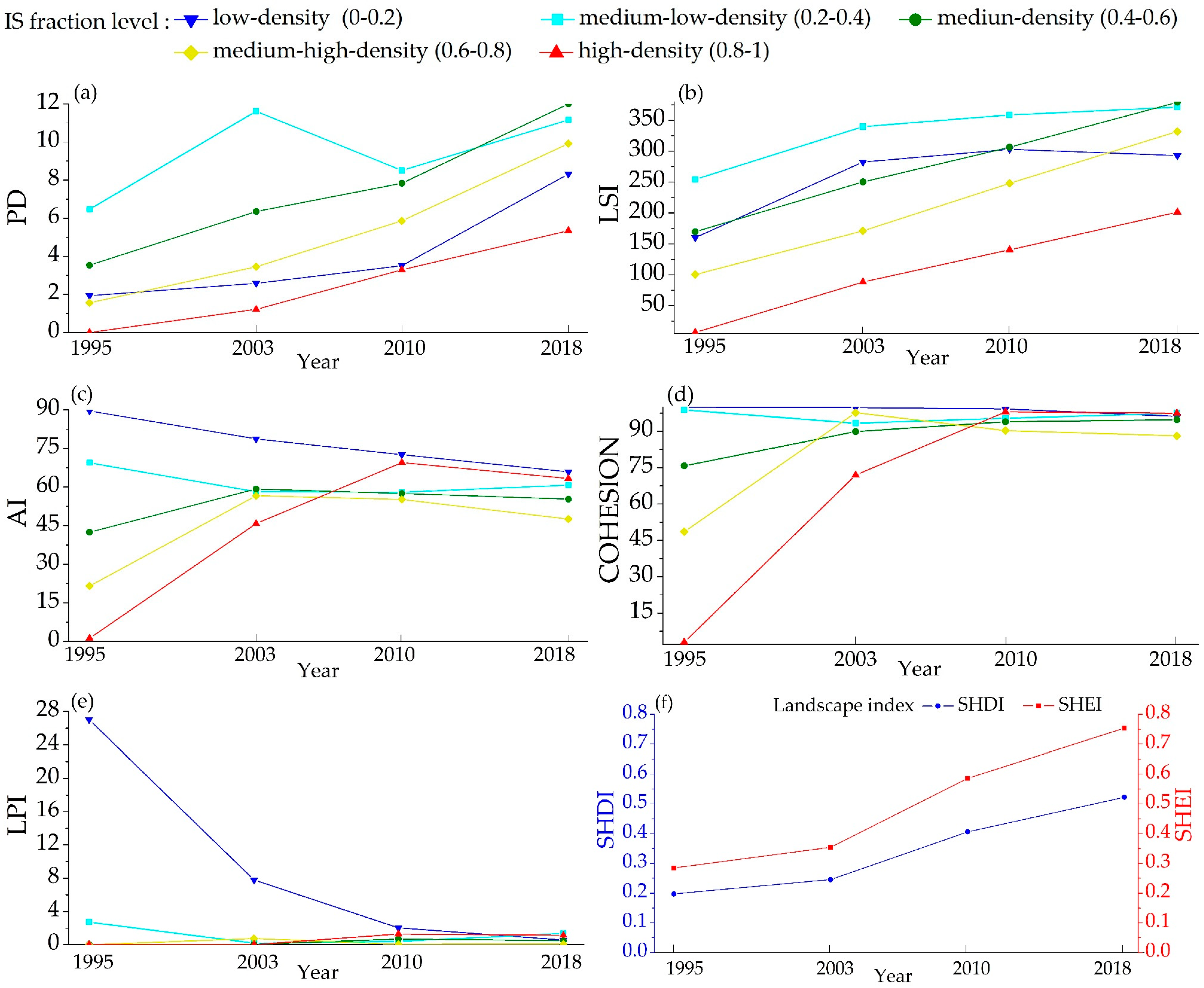
4.2.1. Based on Landscape Indices

Based on the five levels of impervious surface fractions (Section 4.1), landscape indices characterizing impervious surfaces were calculated in Fragstats 4.2 using the method described in Section 3.2. Results are shown in Figure 4.

The PD values gradually increased for all the IS fraction levels except for that for the medium–low-density level (0.2–0.4) which remained the highest with the medium-density level (0.4–0.6) levels (Figure 4a). The LSI values also showed a rising trend for all IS fraction levels except for the low-density level (0–0.2) which saw a gentle decline in 2018 (Figure 4b). Both AI and COHESION values showed similar changes over time (Figure 4c,d). The values for the low-density (0–0.2) and medium–low-density (0.2–0.4) levels decreased gradually while those for the other IS fraction levels rose before going down. The LPI values for the low-density level (0–0.2) decreased remarkably while little change was observed for the other levels (Figure 4e). Regarding the values of landscape-level SHDI and SHEI, both of them increased steadily over the periods (Figure 4f).

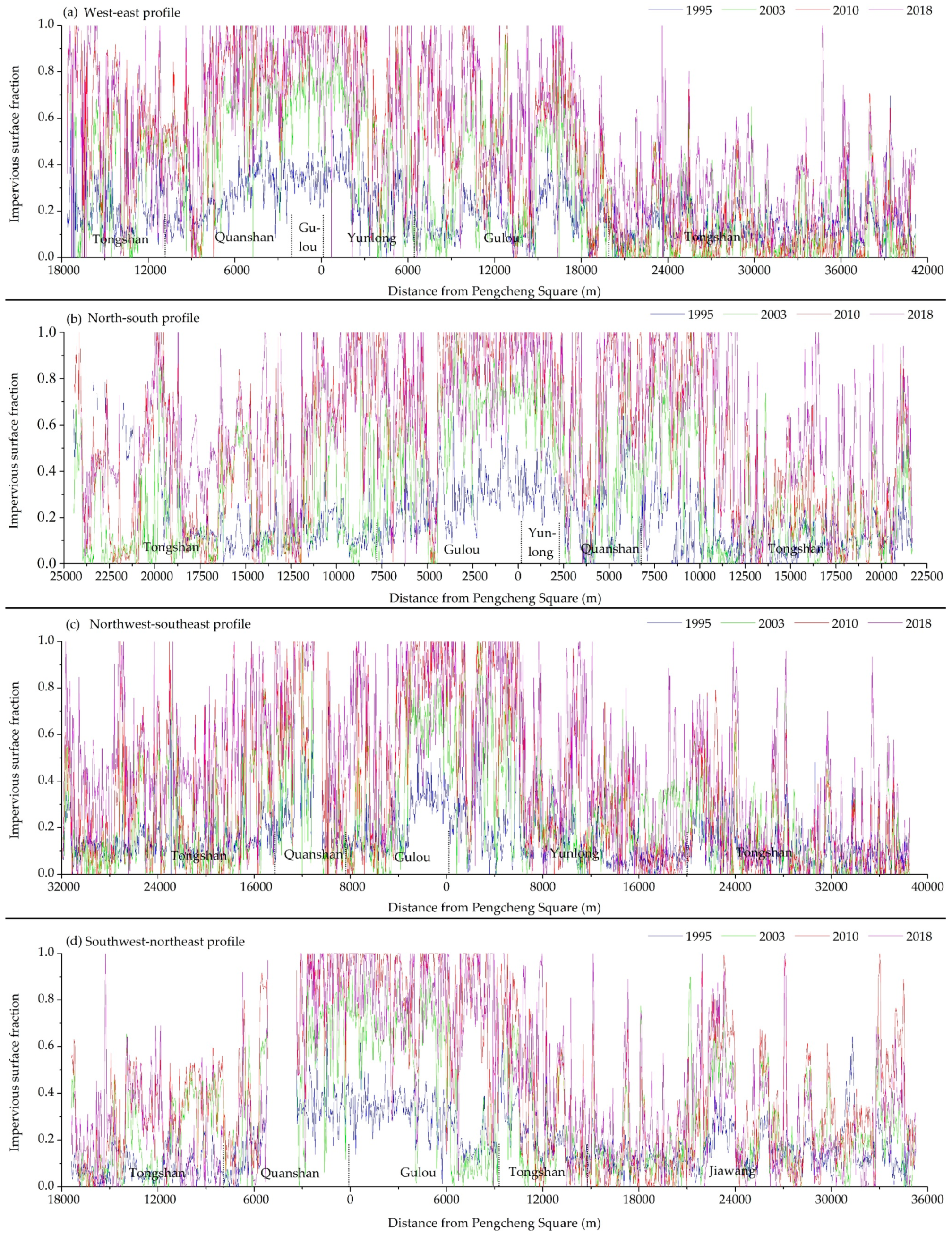
4.2.2. Based on Profile Line Analysis

Analyses in Section 4.1 show that impervious surface expansion varies within the study area. This might be further revealed through profile lines analysis. Along the four profile lines through Pengcheng Square (Figure 1b), we extracted impervious surface fractions for each year (Figure 5).

Along the W–E profile line traveling from Dapeng town and ending with Daxu town in Tongshan district through Quanshan, Gulou, Yunlong, and Gulou district (Figure 5a), impervious surface fractions were lower in the east than those in west. The N–S profile line also started and ended in the Tongshan district through the districts of Gulou, Yunlong, and Quanshan (Figure 5b) reveals that the impervious surface fractions of the CUA were higher than the other areas along the line. The NW–SE profile line that travels from Huangji town to Fangcun town (Figure 5c) also shows the highest impervious surface fractions were focused in Yunlong and Gulou districts, and the lowest in the southeast of Tongshan district. Regarding the SW–NE profile line going through Hanwang town of Tongshan district, Quanshan, Gulou, Tongshan, and Jiawang districts (Figure 5d), impervious surface fractions were clearly higher the CUA than the other areas. From a spatial perspective, the CUAs were constantly observed with the highest impervious surface fractions; from a temporal perspective, impervious surface fractions increased in general over the 23 years, though differently.

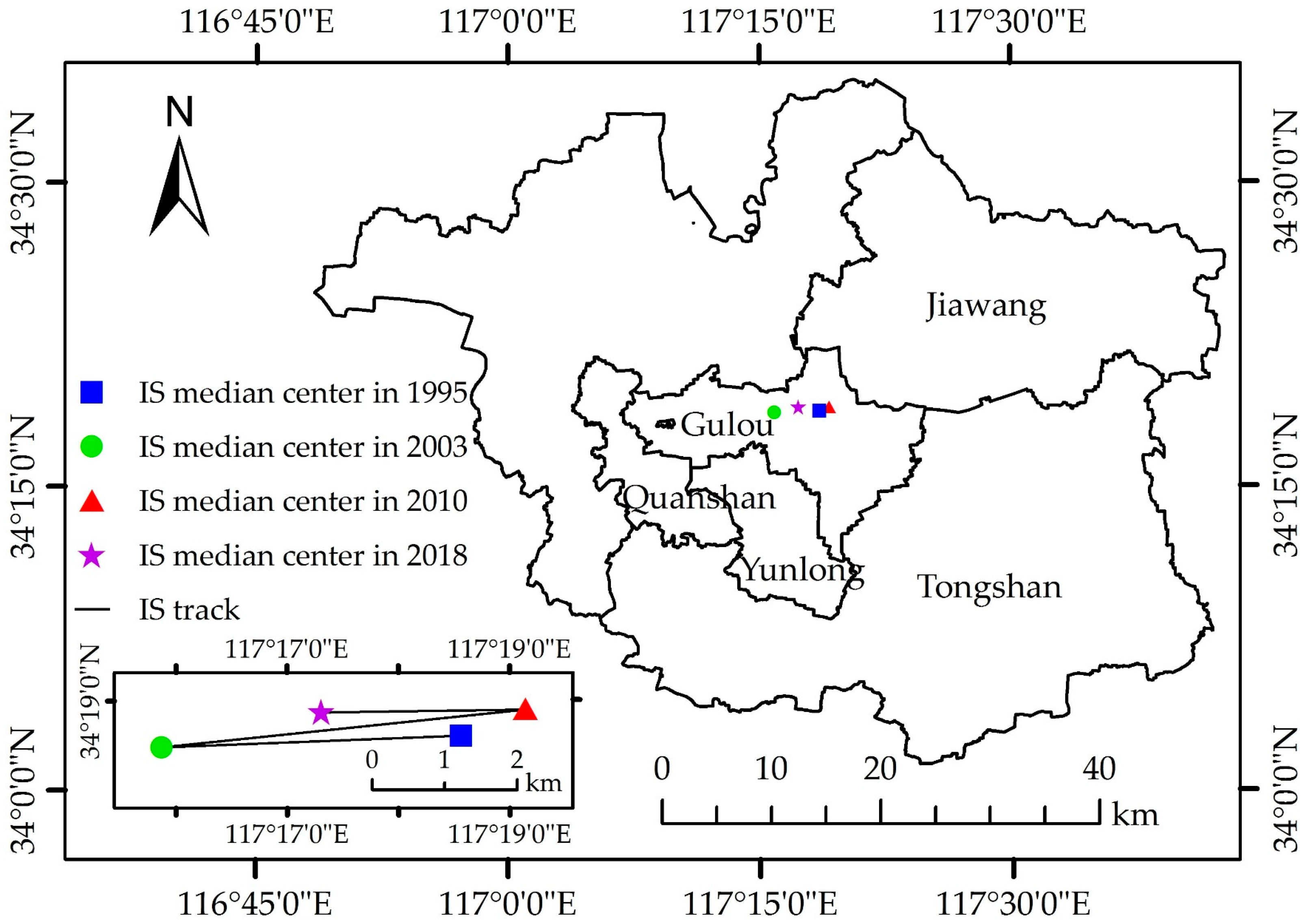
4.2.3. Based on Median Centers and Standard Deviational Ellipses

Following the method described in Section 3.4, the median centers of impervious surfaces were computed, and their tracks were illustrated for both the entire study area (Figure 6) and individual districts (Figure 7). On the city scale, the median centers of the impervious surfaces were located at 117.264° E–117.309° E, 34.311° N–34.316° N during the 23-year period (

Table 4. Changes in impervious surface (IS) median centers from 1995 to 2018.

	Year	Longitude	Latitude	Direction	Distance (m)	Rate (m/Year)
Entire study area	1995	117.309	34.312
	2003	117.264	34.311	South by West 87.614°	4142.326	517.791
	2010	117.319	34.316	North by East 83.962°	5052.360	721.766
	2018	117.288	34.315	South by West 89.203°	2810.981	351.373
Yunlong	1995	117.252	34.227
	2003	117.259	34.219	South by East 34.917°	1139.959	142.495
	2010	117.269	34.211	South by East 46.503°	1309.504	187.072
	2018	117.270	34.208	South by East 12.693°	345.311	43.164
Quanshan	1995	117.144	34.261
	2003	117.128	34.274	North by West 46.015°	2018.026	252.253
	2010	117.128	34.271	South by West 13.069°	311.475	44.496
	2018	117.127	34.272	North by West 16.858°	124.548	15.569
Gulou	1995	117.264	34.299
	2003	117.285	34.298	South by East 84.954°	1929.492	241.187
	2010	117.294	34.296	South by East 77.417°	846.692	120.956
	2018	117.290	34.296	South by West 82.108°	376.160	47.020
Jiawang	1995	117.487	34.377
	2003	117.445	34.384	North by West 79.222°	3930.147	491.268
	2010	117.522	34.386	North by East 87.636°	7069.117	1009.874
	2018	117.481	34.388	North by West 86.840°	3760.815	470.102
Tongshan North	1995	117.127	34.406
	2003	117.117	34.404	South by West 77.015°	935.967	116.996
	2010	117.129	34.410	North by East 61.813°	1282.801	183.257
	2018	117.103	34.416	North by West 72.782°	2511.314	313.914
Tongshan South	1995	117.440	34.176
	2003	117.386	34.157	South by West 66.463°	5426.369	678.296
	2010	117.416	34.175	North by East 54.034°	3481.849	497.407
	2018	117.422	34.173	South by East 74.055°	555.488	69.436

), and shifted nearly horizontally over time. During the 2003 to 2010 period, the annual average movement to the east accelerated. However, the overall moving distance from 1995 to 2018 was relatively small for the entire area (Figure 6), and the overall expansion direction is not significant. On the district scale, however, the median centers of the impervious surfaces in Gulou, Yunlong, and Quanshan districts showed obvious expansion directions, towards the east (Figure 7b), southeast (Figure 7c), and northwest (Figure 7f). Tongshan district shows internal differences, with the expansion directions and distances in Tongshan North were different from those in Tongshan South (Figure 7, Table 4).

The standard deviational ellipses (SDEs) are shown in Figure 8. For the entire study area, the rotation angles ranged from 96.539° to 109.964°, and the long–short axis ratios were all close to one during the 1995 to 2018 period (

Table 5. Standard deviational ellipse (SDE) parameters of impervious surfaces from 1995 to 2018.

	Year	Long Axis (m)	Short Axis (m)	Rotation Angle (°)	Long–Short Axis Ratio
Entire study area	1995	49,554.821	35,044.991	96.881	1.414
	2003	48,531.016	36,450.925	109.964	1.331
	2010	52,697.685	38,485.566	96.539	1.369
	2018	54,209.752	37,594.564	108.895	1.442
Yunlong	1995	13,017.390	5793.510	138.022	2.247
	2003	12,887.834	6033.898	138.903	2.136
	2010	12,320.285	6322.815	146.077	1.949
	2018	12,066.116	6579.798	147.634	1.834
Quanshan	1995	15,301.653	5207.599	142.609	2.938
	2003	16,360.322	5451.560	143.717	3.001
	2010	17,252.284	5450.035	146.524	3.166
	2018	16,248.859	5422.818	144.478	2.996
Gulou	1995	19,318.182	7949.150	94.287	2.430
	2003	19,881.054	8537.040	100.230	2.329
	2010	19,591.029	9552.415	101.992	2.051
	2018	19,955.805	9482.594	101.522	2.104
Jiawang	1995	26,553.175	12,181.719	85.191	2.180
	2003	26,829.005	12,848.135	89.737	2.088
	2010	29,754.558	14,083.920	94.854	2.113
	2018	27,960.891	14,735.358	92.248	1.900
Tongshan North	1995	33,932.906	22,492.496	45.089	1.509
	2003	34,789.711	23,312.088	43.967	1.492
	2010	37,540.409	24,377.139	48.524	1.540
	2018	34,285.429	25,266.912	54.840	1.357
Tongshan South	1995	40,803.393	21,606.868	71.195	1.880
	2003	40,314.726	20,182.057	74.447	1.998
	2010	44,295.083	20,182.057	69.779	2.137
	2018	41,993.619	20,489.428	69.395	2.050

), indicating that the impervious surfaces had no clear expansion direction. The SDEs on the district scale were different from those on the city scale (Figure 8). The long–short axis ratio of each district was significantly larger than that of the entire study area (Table 5), reflecting the obvious expansion direction on the district scale. As the major components of the CUA, Gulou, Yunlong, and Quanshan districts presented expansion towards the east (Figure 8b), southeast (Figure 8c), and northwest (Figure 8f). Such observations on both the city and district scales were consistent with those of the median centers in Figure 7 and Table 4.

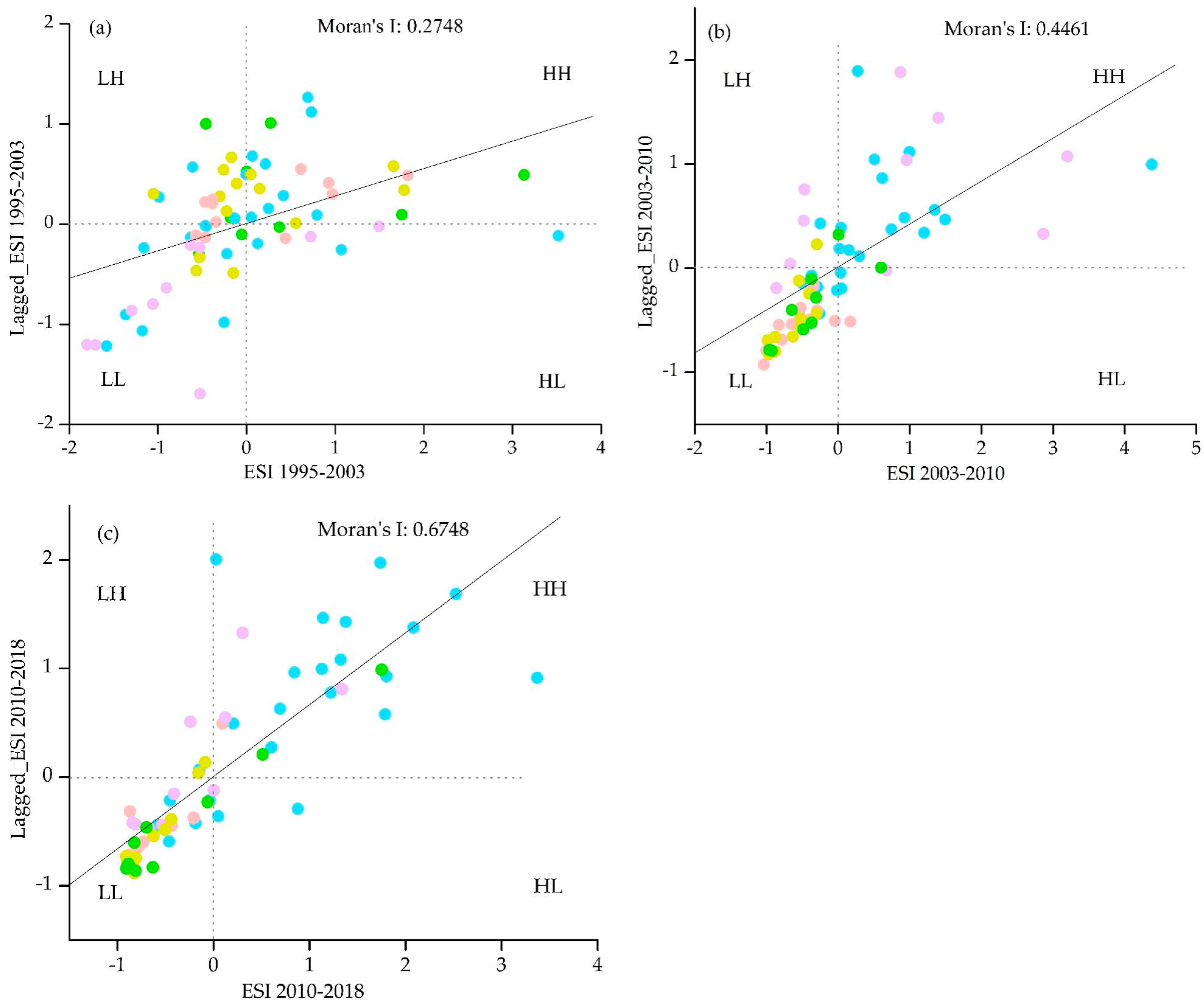
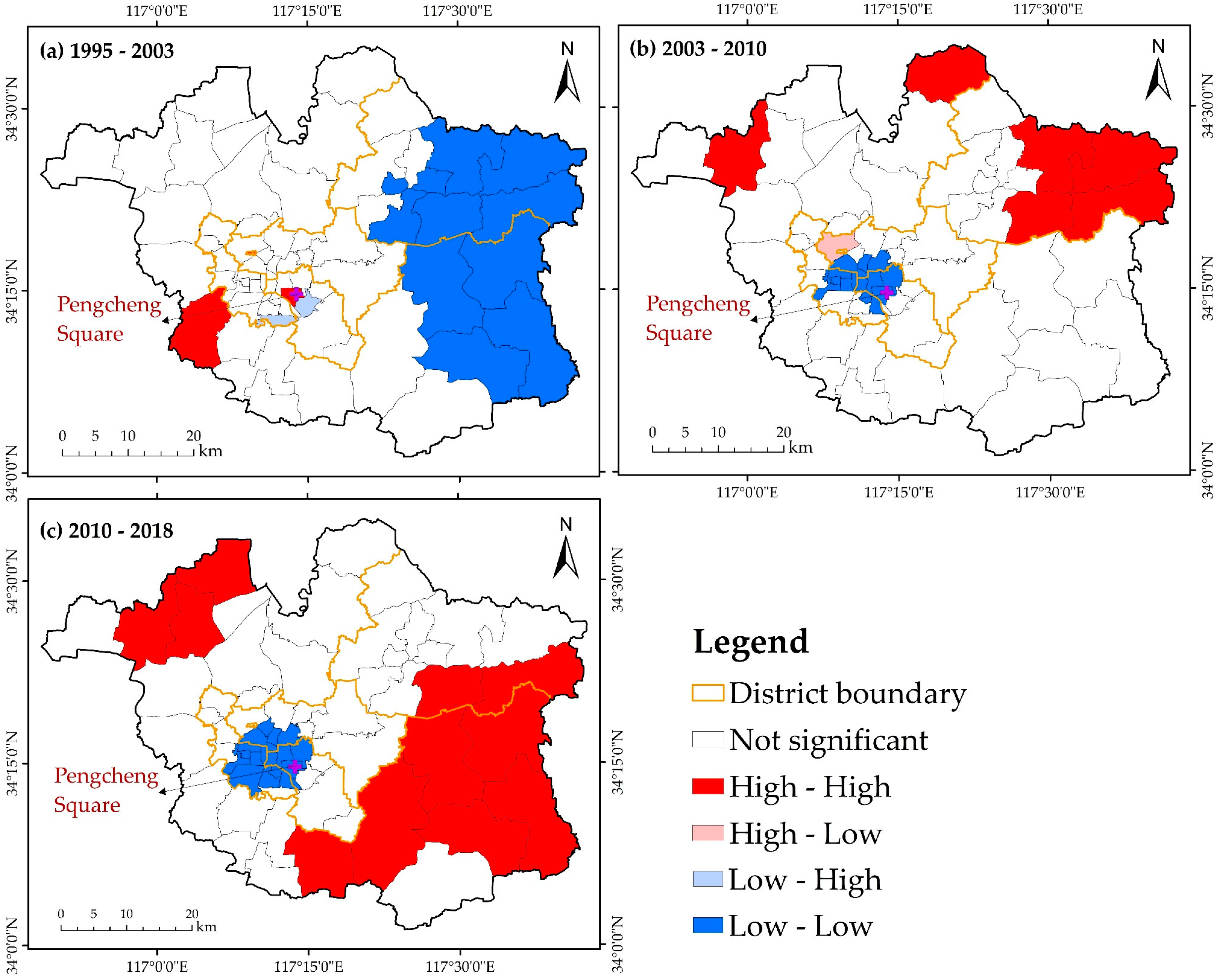
4.2.4. Based on Spatial Autocorrelation Analyses

The expansion speed indices (ESIs) of the impervious surfaces of the entire study area during the 1995–2003, 2003–2010, and 2010–2018 periods were calculated according to Formula (6). Then both global and local spatial autocorrelation analyses were performed to explore their spatial correlations.

The Moran’s I of ESIs was 0.2748, 0.4461, and 0.6748 in 1995–2003, 2003–2010, and 2010–2015, respectively (Figure 9), showing that there were positive autocorrelations in the expansion rates of impervious surfaces. In addition, the Moran’s I gradually increased over time (Figure 9). The towns of ESIs in the three periods were mainly distributed in the HH and LL quadrants, indicating that spatial homogeneity and aggregation pattern of expansion rate were significant. In addition, the towns in the LL quadrants is aggregate, while the towns in the HH quadrants are scattered.

In addition, the LISA cluster maps (Figure 10) were also generated to show the type of towns which passed the significance test. We observed that the HH and LL clustering dominated in the three periods. In the 1995 to 2003 period (Figure 10a), the HH and LH clustering occurred around Pengcheng Square and the LL clustering in Jiawang and Tongshan districts. However, there seemed an opposite trend that LL and HL clustering are distributed around Pengcheng Square for the 2003 to 2010 period (Figure 10b). In the 2010 to 2018 period (Figure 10c), both the HH and LL clustering expanded compared to the previous period.

5. Interpretation and Discussion

In this study, we first mapped urban impervious surfaces of Xuzhou by the LSMA from multi-temporal Landsat image data of 1995, 2003, 2010, and 2018. As urban expansion is a complex process involving landscape pattern, expansion direction, and rate difference, various methods including landscape indices, profile lines, median centers, standard deviational ellipses, and spatial autocorrelation were adopted to characterize the above aspects and comprehensively reflect urban dynamics. The interpretation of the results and their implications are detailed below.

5.1. Overall Dynamics

Impervious surfaces of Xuzhou rose dramatically with rapid urbanization in the recent two decades, as there exists a strong relationship between impervious surface fractions and urban development [61]. The downtown area has always had relatively high impervious surface fractions due to its high socioeconomic level and building density (Figure 2). The rapid development of the CUA has been driving the development of the whole city over time [62] and shows a positive impact on its neighboring towns (Figure 2), a pattern observed in other cities in Asia, such as Tokyo [63] and Shanghai [64]. The transformation of impervious surfaces from low density to high density is a typical feature of rapid urbanization (Figure 3) [65]. In addition, the development of the new urban area (SE Yunlong district) and the construction of transportation facilities in Xuzhou, such as the subway, further promote the overall urbanization, leading to increased impervious surface fractions and a complicated and fragmented trend in the spatial pattern [54], showing the agglomeration effect of urban impervious surfaces. This is because of the implementation of urban renewal projects in Xuzhou—scattered and chaotic buildings have been mostly replaced with continuous residential, commercial, and industrial facilities, leading to increased impervious surface fractions. As there is a negative correlation between impervious surfaces and vegetation [31], low impervious surface fractions were observed in the southeast of the study area where Lvliang Hill Scenic spots was located with abundant vegetation. Balanced development of impervious surface expansion and ecological environment protection contributes to an increased landscape diversity.

Along with urban expansion, vegetation has also flourished in recent years. In the early period, vegetated land was converted to built-up land for constructing residential and commercial buildings. As ecological protection consensus started to emerge, efforts, such as afforestation and ecological restoration for coal mining subsidence areas, have brought more greenness back to Xuzhou in recent years. These measures were also proven effective in other cities [66].

5.2. Landscape Pattern

An increase in PD indicates increasing landscape heterogeneity of impervious surfaces (Figure 4a). The advancement of urbanization has made impervious surfaces expand outside with a large number of residential areas scattered in the suburbs, leading to an increasing fragmentation trend of impervious surfaces. The increase in the LSI (Figure 4b) also indicates that the spatial pattern of impervious surfaces is irregular and complicated. In addition, the establishment of industrial zones, the development of the new urban areas (SE Yunlong district) and the construction of transportation facilities in Xuzhou, such as subways, further promoted the overall urbanization, making the original landscape pattern more complex and fragmented [54,65]. The changes in AI and COHESION (Figure 4c,d) indicate that the low- and medium–low-density impervious surfaces exhibited a dispersive expansion and the connectivity was reduced. This is because the promotion of eco–environmental protection, such as the construction of scenic spots, made the impervious surfaces with low density become fragmented and irregular. While the impervious surfaces with high density showed a filled expansion and enhanced connectivity, which is closely related to the transformation of the old city in Xuzhou, the LPI of the low-density impervious surface dramatically reduced (Figure 4e), indicating that urbanization made its dominance significantly reduce, and part of it was gradually occupied by high-density [65], which is the inevitable result of urban expansion.

At the landscape level, gradually increased SHDI and SHEI (Figure 4f), suggest enhanced heterogeneity and landscape diversity. This is because urbanization has reduced the dominance of agricultural land and vegetation by converting part of them into impervious surfaces. Meanwhile, there are some open green spaces in the study area, such as Yunlong Mountain scenic area, Quanshan forest park, and Jiulihu wetland park, and large-area water landscapes, such as Yunlong Lake and Dalong Lake. These permeable landscapes are important for maintaining the original components and the quality of urban ecological environment [67,68]. Coordinated development of impervious surface expansion and eco–environment protection means the landscape types are in a relatively balanced state and increases landscape diversity.

5.3. Expansion Direction

Profile lines, median centers, and SDEs are widely used to characterize urban expansion [14,39]. While Xu et al. (2018) [39] found that the expansion direction of Guangzhou was significantly contrasting on the whole and local region scale, we found Xuzhou featured different expansion directions than Guangzhou.

In this study, the impervious surfaces did not exhibit an obvious expansion direction on the city scale (Figure 6 and Figure 8). The annual average rate of expansion to the east has increased during the 2003 to 2010 period (Table 4) probably resulted from a governmental policy—the Xuzhou Eleventh Five-Year Plan (2006–2010) had clearly stated Xuzhou would expand eastward. However, this was not significant for the entire study area from 1995 to 2018. On the district scale (Figure 5, Figure 6, Figure 7 and Figure 8), Quanshan, Gulou, and Yunlong districts, the major components of the CUA, have increasingly high impervious surface fractions, which is related to their urbanization that started early and developed rapidly. The impervious surfaces of Quanshan district expanded towards the northwest before the Pangzhuang mine was closed in Pangzhuang town in the NW Quanshan district. While coal mining related subsidence was a serious issue in Pangzhuang town, the government encouraged the expansion of the CUA towards east and southeast, e.g., building a key high-speed railway station in east Gulou district and creating the Xuzhou national economic development zone covering east CUA, relocating government offices to the new urban area in SE Yunlong district. These expansion directions are consistent with the requirements of the Xuzhou General Urban Planning (2007-2020) that built-up land in the CUA should be developed in the east and southeast, be controlled in the northwest, and strictly restricted in the southwest [69].

5.4. Expansion Rate

The expansion rates of impervious surfaces during the two decades were shown to have significant spatial autocorrelation, and the spatial agglomeration gradually increased with the advancement of urbanization (Figure 9). HH and LL clustering of impervious surface expansion dominated in Xuzhou, the central city of the Huaihai Economic Zone (Figure 9), as urban development in economic regions tends to be homogeneous [70].

The urbanization of the downtown area started early, showing HH and LH clustering around Pengcheng Square in the 1995 to 2003 period (Figure 10a). Note that the clustering only implies a relative change, rather than an absolute value difference [14]. LH clustering does not necessarily mean that the towns in this type have a low expansion rate, but tells us that their neighboring towns’ impervious surfaces expand faster. In the periods of 2003 to 2010 and 2010 to 2018, opposite spatial distributions were observed with the LL and LH clustering occurring in the downtown area (Figure 10b,c), which is due to the fact that the development of downtown area slowed down relatively after approaching saturation. Likewise, the town shown as HL clustering expanded relatively faster because of their proximity to the saturated downtown area (Figure 10b). In addition, Tongshan and Jiawang, which are not included in the CUA, developed late, but their urbanization has accelerated in recent years (Figure 10b,c). Tongshan district developed rapidly, upgrading from a rural county to an urban district. This explains why LL clustering appeared in the downtown area, and HH clustering were in the suburbs. However, because of unevenly natural resource distribution [71] and the effect of government policies, expansion rate varied in the towns largely within Tongshan district (Table 4), with the HH clustering in different locations (Figure 10c).

5.5. Innovation and Limitation

Studies of the spatiotemporal dynamics of impervious surfaces on either region or city scale are important for understanding the overall pattern and development model [33,34,35,36]. However, these may fail to notice the variation among the areas of lower administrative levels in regional development [72,73,74]. A better characterization of the spatiotemporal dynamics of impervious surfaces entails perspectives on different scales in the case study of Xuzhou. In addition, although a single method may unravel a certain aspect of urban development [39,41], this is overshadowed by the complexity of urban development [75]. The combination of many different methods together with analyses on different scales, as demonstrated in our case study, provides a new perspective for comprehensive quantification of urban expansion.

However, we here would like to raise the issue of discriminating endmembers in the process of endmember selection in this study. While vegetation is most detectable and low-albedo impervious surfaces exist in large amounts in urban areas, it is challenging to identify high-albedo impervious surfaces, and bare soil endmembers as both of them are usually uncommon in cities. Moreover, because they are quite similar in spectral characteristics, high-albedo impervious surfaces could be easily confused with bare soil. As such, an increased resolution of image data and a more advanced endmember extraction procedure would improve the accuracy of mapping impervious surfaces.

6. Conclusions

This study characterizes and analyzes the spatiotemporal dynamics of impervious surfaces of Xuzhou from 1995 to 2018 on different scales using various and complementary methods. The key findings and main conclusions are summarized as follows:

• Impervious surfaces increased obviously in the context of rapid urbanization, which changed urban landscape patterns. Impervious surfaces with high fractions were mainly concentrated in the downtown area, showing an expansion starting from the downtown area. Impervious surfaces were generally fragmented and irregular. Meanwhile, vegetation also flourished in recent years. Scientific urban planning promotes the balanced development of impervious surface expansion and ecological environmental protection, increasing the diversity of landscape.
• Significant differences in the expansion direction of impervious surfaces existed in the entire study area and each district. The expansion direction of the study area was not obvious, while the districts within the CUA shows clear expansion directions towards the east and southeast, which is consistent with the general urban planning. Therefore, more importance should be placed on the urban planning and policy guidance to stimulate and regulate the overall orderly urban development.
• Expansion rates of impervious surfaces showed a significant spatial agglomeration, which increased gradually and varied with the town. The urbanization of the downtown area started early and has gradually become saturated, while the non-CUA accelerated its development with the large internal differences. This suggests that resource distribution and government policies affect urban expansion rates.

Findings from this study will be helpful to understand the tempo–spatial variation in urban expansion, providing a basis for analyzing its environmental effects and exploring its driving mechanism. Moreover, this will contribute to decision-makers in formulating urban planning policies and provides a reference for similar studies.

References

1. Maggiore, G.; Semeraro, T.; Aretano, R.; De Bellis, L.; Luvisi, A. GIS analysis of land-use change in threatened landscapes by Xylella fastidiosa. Sustainability 2019, 11, 253. [Google Scholar] [CrossRef]
2. Yu, X.; Zhang, B.; Li, Q.; Chen, J. A method characterizing urban expansion based on land cover map at 30 m resolution. Earth Sci. 2016, 59, 1738–1744. [Google Scholar] [CrossRef]
3. Arribas-bel, D.; Nijkamp, P.; Scholten, H. Multidimensional urban sprawl in Europe: A self-organizing map approach. Comput. Environ. Urban Syst. 2011, 35, 263–275. [Google Scholar] [CrossRef] [Green Version]
4. Liu, X.; Li, X.; Chen, Y.; Tan, Z.; Li, S.; Ai, B. A new landscape index for quantifying urban expansion using multi-temporal remotely sensed data. Landsc. Ecol. 2010, 25, 671–682. [Google Scholar] [CrossRef]
5. Jiao, L.; Mao, L.; Liu, Y. Multi-order landscape expansion index: Characterizing urban expansion dynamics. Landsc. Urban Plan. 2015, 137, 30–39. [Google Scholar] [CrossRef]
6. Torbick, N.; Corbiere, M. Mapping urban sprawl and impervious surfaces in the northeast United States for the past four decades. GISci. Remote Sens. 2015, 52, 746–764. [Google Scholar] [CrossRef]
7. Ma, L.; Zhao, H.; Li, J. Examining urban expansion using multi-temporal Landsat imagery: A case study of the Montreal census metropolitan area from 1975 to 2015, Canada. ISPRS J. Photogramm. Remote Sens. 2016, XLI-B8, 965–972. [Google Scholar]
8. Adhikari, P.; Beurs, K.M. De Growth in urban extent and allometric analysis of West African cities. J. Land Use Sci. 2017, 12, 105–124. [Google Scholar] [CrossRef]
9. Di Palma, F.; Amato, F.; Nolè, G.; Martellozzo, F.; Murgante, B. A SMAP supervised classification of Landsat images for urban sprawl evaluation. Int. J. Geo-Inf. 2016, 5, 109. [Google Scholar] [CrossRef]
10. Shafizadeh-moghadam, H.; Tayyebi, A.; Helbich, M. Transition index maps for urban growth simulation: Application of artificial neural networks, weight of evidence and fuzzy multi-criteria evaluation. Environ. Monit. Assess. 2017, 189, 300. [Google Scholar] [CrossRef] [PubMed]
11. Devendran, A.A.; Lakshmanan, G. Urban growth prediction using neural network coupled agents-based Cellular Automata model for Sriperumbudur Taluk, Tamil Nadu, India. Egypt. J. Remote Sens. Space Sci. 2018, 21, 353–362. [Google Scholar]
12. Wang, L.; Li, C.C.; Ying, Q.; Cheng, X.; Wang, X.Y.; Li, X.Y.; Hu, L.Y.; Liang, L.; Yu, L.; Huang, H.B.; et al. China’s urban expansion from 1990 to 2010 determined with satellite remote sensing. Chin. Sci. Bull. 2012, 57, 2802–2812. [Google Scholar] [CrossRef] [Green Version]
13. Kuang, W.; Chi, W.; Lu, D.; Dou, Y. A comparative analysis of megacity expansions in China and the U.S.: Patterns, rates and driving forces. Landsc. Urban Plan. 2014, 132, 121–135. [Google Scholar] [CrossRef]
14. Peng, J.; Liu, Y.; Shen, H.; Xie, P.; Hu, X.; Wang, Y. Using impervious surfaces to detect urban expansion in Beijing of China in 2000s. Chin. Geogr. Sci. 2016, 26, 229–243. [Google Scholar]
15. Xu, H. Analysis of impervious surface and its impact on urban heat environment using the normalized difference impervious surface index (NDISI). Photogramm. Eng. Remote Sens. 2010, 76, 557–565. [Google Scholar] [CrossRef]
16. Liu, C.; Shao, Z.; Chen, M.; Luo, H. MNDISI: A multi-source composition index for impervious surface area estimation at the individual city scale. Remote Sens. Lett. 2013, 4, 803–812. [Google Scholar] [CrossRef]
17. Lu, D.; Hetrick, S.; Moran, E. Impervious surface mapping with Quickbird imagery. Int. J. Remote Sens. 2011, 32, 2519–2533. [Google Scholar] [CrossRef] [PubMed] [Green Version]
18. Wu, C. Normalized spectral mixture analysis for monitoring urban composition using ETM+ imagery. Remote Sens. Environ. 2004, 93, 480–492. [Google Scholar] [CrossRef]
19. Yuan, F.; Bauer, M.E. Comparison of impervious surface area and normalized difference vegetation index as indicators of surface urban heat island effects in Landsat imagery. Remote Sens. Environ. 2007, 106, 375–386. [Google Scholar] [CrossRef]
20. Anindita, S.C.; Prafull, S.; Rai, S.C. Assessment of impervious surface growth in urban environment through remote sensing estimates. Environ. Earth Sci. 2017, 76, 1–14. [Google Scholar]
21. De Asis, A.M.; Omasa, K. Estimation of vegetation parameter for modeling soil erosion using linear spectral mixture analysis of Landsat ETM data. Photogramm. Remote Sen. 2007, 62, 309–324. [Google Scholar] [CrossRef]
22. Zhang, Y.; Li, L.; Qin, K.; Wang, Y. Remote sensing estimation of urban surface evapotranspiration based on a modified Penman–Monteith model. J. Appl. Remote Sens. 2018, 12, 046006. [Google Scholar] [CrossRef]
23. Sun, D.; Liu, N. Coupling spectral unmixing and multiseasonal remote sensing for temperate dryland land-use/land-cover mapping in Minqin County, China. Int. J. Remote Sens. 2015, 36, 3636–3658. [Google Scholar] [CrossRef]
24. Schmitt-harsh, M.; Sweeney, S.P.; Evans, T.P. Classification of coffee-forest landscapes using Landsat TM imagery and spectral mixture analysis. Photogramm. Eng. Remote Sens. 2013, 79, 457–468. [Google Scholar] [CrossRef]
25. Siregar, V.P.; Prabowo, N.W. Linear spectral mixture analysis of SPOT-7 for tea yield estimation in Pagilaran Estate, Batang Central Java. Earth Environ. Sci. 2016, 47, 012034. [Google Scholar]
26. Yan, E.; Lin, H.; Wang, G.; Sun, H. Improvement of forest carbon estimation by integration of regression modeling and spectral unmixing of Landsat data. IEEE Geosci. Remote Sens. Lett. 2015, 12, 2003–2007. [Google Scholar]
27. Kawakubo, F.S.; Paul, R.; Machado, P. Mapping coffee crops in southeastern Brazil using spectral mixture analysis and data mining classification. Int. J. Remote Sens. 2016, 37, 3414–3436. [Google Scholar] [CrossRef]
28. Li, L.; Canters, F.; Solana, C.; Ma, W.; Chen, L.; Kervyn, M. Discriminating lava flows of different age within Nyamuragira’s volcanic field using spectral mixture analysis. Int. J. Appl. Earth Obs. Geoinf. 2015, 40, 1–10. [Google Scholar] [CrossRef] [Green Version]
29. Tang, F.; Xu, H. Impervious surface information extraction based on hyperspectral remote sensing imagery. Remote Sens. 2017, 9, 550. [Google Scholar] [CrossRef]
30. Voorde, T.V.D.; Roeck, T.D.; Canters, F. A comparison of two spectral mixture modelling approaches for impervious surface mapping in urban areas. Int. J. Remote Sens. 2009, 30, 4785–4806. [Google Scholar] [CrossRef]
31. Ridd, M.K. Exploring a V-I-S (vegetation-impervious surface-soil) model for urban ecosystem analysis through remote sensing: Comparative anatomy for cities. Int. J. Remote Sens. 1995, 16, 2165–2185. [Google Scholar] [CrossRef]
32. Deák, M.; Telbisz, T.; Árvai, M.; Mari, L.; Horváth, F.; Kohán, B.; Szabó, O.; Kovács, J. Heterogeneous forest classification by creating mixed vegetation classes using EO-1 Hyperion. Int. J. Remote Sens. 2017, 38, 5215–5231. [Google Scholar]
33. Gao, F.; De Colstoun, E.B.; Ma, R.; Weng, Q.; Masek, J.G.; Chen, J.; Pan, Y.; Song, C. Mapping impervious surface expansion using medium-resolution satellite image time series: A case study in the Yangtze River Delta, China. Int. J. Remote Sens. 2012, 33, 7609–7628. [Google Scholar] [CrossRef]
34. Zhang, L.; Weng, Q. Annual dynamics of impervious surface in the Pearl River Delta, China, from 1988 to 2013, using time series Landsat imagery. ISPRS J. Photogramm. Remote Sens. 2016, 113, 86–96. [Google Scholar] [CrossRef]
35. Seto, K.C.; Fragkias, M. Quantifying spatiotemporal patterns of urban land-use change in four cities of China with time series landscape metrics. Landsc. Ecol. 2005, 20, 871–888. [Google Scholar] [CrossRef]
36. Li, X.; Gong, P.; Liang, L. A 30-year (1984–2013) record of annual urban dynamics of Beijing City derived from Landsat data. Remote Sens. Environ. 2015, 166, 78–90. [Google Scholar] [CrossRef]
37. Luck, M.; Wu, J. A gradient analysis of urban landscape pattern: A case study from the Phoenix metropolitan region, Arizona, USA. Landsc. Ecol. 2002, 17, 327–339. [Google Scholar] [CrossRef]
38. Zhou, W.; Huang, G.; Pickett, S.T.A.; Cadenasso, M.L. 90 Years of forest cover change in an urbanizing watershed: Spatial and temporal dynamics. Landsc. Ecol. 2011, 26, 645–659. [Google Scholar] [CrossRef]
39. Xu, J.; Zhao, Y.; Zhong, K.; Zhang, F.; Liu, X.; Sun, C. Measuring spatio-temporal dynamics of impervious surface in Guangzhou, China, from 1988 to 2015, using time-series Landsat imagery. Sci. Total Environ. 2018, 627, 264–281. [Google Scholar] [CrossRef] [PubMed]
40. Kowe, P.; Pedzisai, E.; Gumindoga, W.; Rwasoka, D.T. An analysis of changes in the urban landscape composition and configuration in the Sancaktepe District of Istanbul Metropolitan City, Turkey using landscape metrics and satellite data. Geocarto Int. 2015, 30, 506–519. [Google Scholar] [CrossRef]
41. Hu, D.; Wu, Y.; Li, X. Research on the space linking up Changsha-Zhuzhou-Xiangtan under the background of environmental-friendly society. Appl. Mech. Mater. 2012, 174–177, 2529–2532. [Google Scholar] [CrossRef]
42. Zhang, Y.; Chen, L.; Wang, Y.; Chen, L.; Yao, F.; Wu, P.; Wang, B.; Li, Y.; Zhou, T.; Zhang, T. Research on the contribution of urban land surface moisture to the alleviation effect of urban land surface heat based on Landsat 8 data. Remote Sens. 2015, 7, 10737–10762. [Google Scholar] [CrossRef]
43. Pan, J.; Wang, M.; Li, D. Automatic generation of seamline network using area voronoi diagrams with overlap. IEEE Trans. Geosci. Remote Sens. 2009, 47, 1737–1744. [Google Scholar] [CrossRef]
44. Chen, Y.; Yu, S. Assessment of urban growth in Guangzhou using multi-temporal, multi-sensor Landsat data to quantify and map impervious surfaces. Int. J. Remote Sens. 2016, 37, 5936–5952. [Google Scholar] [CrossRef]
45. Balázs, B.; Bíró, T.; Dyke, G.; Singh, S.K.; Szabó, S. Extracting water-related features using reflectance data and principal component analysis of Landsat images. Hydrol. Sci. J. 2018, 63, 269–284. [Google Scholar] [CrossRef]
46. Szabó, S.; Gácsi, Z.; Balázs, B. Specific features of NDVI, NDWI and MNDWI as reflected in land cover categories. Landsc. Environ. 2016, 10, 194–202. [Google Scholar] [CrossRef]
47. Small, C. The Landsat ETM+ spectral mixing space. Remote Sens. Environ. 2004, 93, 1–17. [Google Scholar] [CrossRef]
48. Congalton, R.G. A review of assessing the accuracy of classifications of remotely sensed data. Remote Sens. Environ. 1991, 37, 35–46. [Google Scholar] [CrossRef]
49. Li, L.; Solana, C.; Canters, F.; Kervyn, M. Testing random forest classification for identifying lava flows and mapping age groups on a single Landsat 8 image. J. Volcanol. Geotherm. Res. 2017, 345, 109–124. [Google Scholar] [CrossRef]
50. Fan, F.; Fan, W.; Weng, Q. Improving urban impervious surface mapping by linear spectral mixture analysis and using spectral indices. Can J. Remote Sens. 2015, 41, 577–586. [Google Scholar] [CrossRef]
51. Weng, Q.; Hu, X.; Liu, H. Estimating impervious surfaces using linear spectral mixture analysis with multitemporal ASTER images. Int. J. Remote Sens. 2009, 30, 4807–4830. [Google Scholar] [CrossRef]
52. Cui, Y.; Li, L.; Chen, L.; Zhang, Y.; Cheng, L.; Zhou, X.; Yang, X. Land-use carbon emissions estimation for the Yangtze River Delta Urban Agglomeration using 1994-2016 Landsat image data. Remote Sens. 2018, 10, 1334. [Google Scholar] [CrossRef]
53. Szabó, S.; Bertalan, L.; Kerekes, Á.; Novák, T.J. Possibilities of land use change analysis in a mountainous rural area: A methodological approach. Int. J. Geogr. Inf. Sci. 2016, 30, 708–726. [Google Scholar] [CrossRef]
54. Fan, F.; Fan, W. Understanding spatial-temporal urban expansion pattern (1990–2009) using impervious surface data and landscape indexes: A case study in Guangzhou (China). J. Appl. Remote Sens. 2014, 8, 083609. [Google Scholar] [CrossRef]
55. Szabó, S.; Csorba, P.; Szilassi, P. Tools for landscape ecological planning—Scale, and aggregation sensitivity of the contagion type landscape metric indices. Carpathian J. Earth Environ. Sci. 2012, 7, 127–136. [Google Scholar]
56. Jaeger, J.A.G. Landscape division, splitting index, and effective mesh size: New measures of landscape fragmentation. Landsc. Ecol. 2000, 15, 115–130. [Google Scholar] [CrossRef]
57. Sha, M.; Tian, G. An analysis of spatiotemporal changes of urban landscape pattern in Phoenix metropolitan region. Procedia Environ. Sci. 2010, 2, 600–604. [Google Scholar] [CrossRef] [Green Version]
58. McGarigal, K.; Cushman, S.A.; Neel, M.C.; Ene, E. Fragstats: Spatial Pattern Analysis Program for Categorical Maps. Available online: http://www.umass.edu/landeco/research/fragstats/fragstats.html (accessed on 26 January 2019).
59. Jia, Y.; Tang, L.; Wang, L. Influence of ecological factors on estimation of impervious surface area using Landsat 8 imagery. Remote Sens. 2017, 9, 751. [Google Scholar] [CrossRef]
60. Yi, F.; Li, R.; Chang, B.; Qiu, J. Spatial-temporal features of construction land expansion in Changzhutan (Changsha-Zhuzhou-Xiangtan) area based on remote sensing. Remote Sens. Land Resour. 2015, 27, 160–166. (In Chinese) [Google Scholar]
61. Shahtahmassebi, A.R.; Song, J.; Zheng, Q.; Blackburn, G.A.; Wang, K.; Huang, L.; Pan, Y.; Moore, N.; Shahtahmassebi, G.; Haghighi, R.S.; et al. Remote sensing of impervious surface growth: A framework for quantifying urban expansion and re-densification mechanisms. Int. J. Appl. Earth Obs. Geoinf. 2016, 46, 94–112. [Google Scholar] [CrossRef] [Green Version]
62. Hollar, M.K. Central cities and susurbs: Economic rivals or allies? J. Reg. Sci. 2011, 51, 231–252. [Google Scholar] [CrossRef]
63. André, S. Land readjustment and metropolitan growth: An examination of suburban land development and urban sprawl in the Tokyo metropolitan area. Prog. Plan. 2000, 53, 217–330. [Google Scholar]
64. Yin, J.; Yin, Z.; Zhong, H.; Xu, S.; Hu, X.; Wang, J.; Wu, J. Monitoring urban expansion and land use/land cover changes of Shanghai metropolitan area during the transitional economy (1979–2009) in China. Environ. Monit. Assess. 2011, 177, 609–621. [Google Scholar] [CrossRef] [PubMed]
65. Zhang, Y.; Xu, B. Spatiotemporal analysis of land use/cover changes in Nanchang area, China. Int. J. Digit. Earth 2015, 8, 312–333. [Google Scholar] [CrossRef]
66. Hu, Z.; Fu, Y.; Xiao, W.; Zhao, Y.; Wei, T. Ecological restoration plan for abandoned underground coal mine site in Eastern China. Int. J. Min. Reclam. Environ. 2015, 29, 316–330. [Google Scholar] [CrossRef]
67. Hüse, B.; Szabó, S.; Deák, B.; Tóthmérész, B. Mapping an ecological network of green habitat patches and their role in maintaining urban biodiversity in and around Debrecen city (Eastern Hungary). Land Use Policy 2016, 57, 574–581. [Google Scholar] [CrossRef]
68. Takács, D.; Varró, D.K.; Bakay, E. Comparison of different space indexing methods for ecological evaluation of urban open spaces. Appl. Ecol. Environ. Res. 2014, 12, 1027–1048. [Google Scholar] [CrossRef]
69. Wu, C.; Pei, F.; Zhou, Y.; Wang, K.; Xu, L. Delineating urban growth boundary from perspective of “negative planning”: A case study of the central urban district in Xuzhou. Geogr. Geo-Inf. Sci. 2017, 33, 92–98. (In Chinese) [Google Scholar]
70. Cao, S.; Hu, D.; Hu, Z.; Zhao, W.; Chen, S.; Yu, C. Comparison of spatial structures of urban agglomerations between the Beijing-Tianjin-Hebei and Boswash based on the subpixel-level impervious surface coverage product. J. Geogr. Sci. 2018, 28, 306–322. [Google Scholar] [CrossRef]
71. Crutzen, B.S.Y.; Holton, S. The more the merrier? Natural resource fragmentation and the wealth of nations. Kyklos 2011, 64, 500–515. [Google Scholar] [CrossRef]
72. Sexton, J.O.; Song, X.P.; Huang, C.; Channan, S.; Baker, M.E.; Townshend, J.R. Urban growth of the Washington, D.C.-Baltimore, MD metropolitan region from 1984 to 2010 by annual, Landsat-based estimates of impervious cover. Remote Sens. Environ. 2013, 129, 42–53. [Google Scholar] [CrossRef]
73. Mu, J. The study on evaluating urban development level and regional difference based on a competitiveness model. J. Appl. Remote Sens. 2013, 13, 5527–5532. [Google Scholar]
74. Liu, J.; Zhang, Q.; Hu, Y. Regional differences of China’s urban expansion from late 20th to early 21st century based on remote sensing information. Chin. Geogr. Sci. 2012, 22, 1–14. [Google Scholar] [CrossRef]
75. Rafiee, R.; Mahiny, A.S.; Khorasani, N.; Darvishsefat, A.A.; Danekar, A. Simulating urban growth in Mashad City, Iran through the SLEUTH model (UGM). Cities 2009, 26, 19–26. [Google Scholar] [CrossRef]
Figure 1. Study area: (a) study area in Jiangsu province; (b) study area consisting of 68 towns (full names tabulated in Table 1), nine in Yunlong, ten in Jiawang, 11 in Gulou, 14 in Quanshan, and 24 in Tongshan district. The purple lines indicate the profile lines used in Section 3.3. The orange line in Tongshan district illustrates the division of this district used in Section 3.4.
Sustainability 11 01224 g001
Figure 2. Impervious surface (IS) fraction maps of 1995, 2003, 2010, and 2018.
Sustainability 11 01224 g002
Figure 3. Number of pixels of different levels of impervious surface fractions in different years (blue for 1995, green for 2003, red for 2010, and violet for 2018).
Sustainability 11 01224 g003
Figure 4. The landscape indices of impervious surface fraction levels from 1995 to 2018. (a) PD. (b) LSI. (c) AI. (d) COHESION. (e) LPI. (f). SHDI.
Sustainability 11 01224 g004
Figure 5. Variation of impervious surface fractions in different years along different profile lines. Colors of the curves refer to the impervious surfaces of different years (blue for 1995, green for 2003, red for 2010, and violet for 2018). The break part in (d) in Quanshan district is the Yunlong Lake which was masked out.
Sustainability 11 01224 g005
Figure 6. IS median centers for the entire study area from 1995 to 2018.
Sustainability 11 01224 g006
Figure 7. IS median centers for each district from 1995 to 2018.
Sustainability 11 01224 g007
Figure 8. Standard deviational ellipses (SDEs) of impervious surfaces from 1995 to 2018.
Sustainability 11 01224 g008
Figure 9. Moran’s I scatter plots of expansion speed indices (ESI) for each town in the different periods: (a) 1995–2003; (b) 2003–2010; and (c) 2010–2018. Green, yellow, rose, lilac and blue represent the towns of Yunlong, Quanshan, Gulou, Jiawang, and Tongshan districts, respectively.
Sustainability 11 01224 g009
Figure 10. Local indicators of spatial association (LISA) cluster maps of ESI for each town in the different periods: (a) 1995–2003; (b) 2003–2010; and (c) 2010–2018.
Sustainability 11 01224 g010