Hydrological Responses to Climate and Land Use Changes in a Watershed of the Loess Plateau, China

Abstract

This study researched the individual and combined impacts of future LULC and climate changes on water balance in the upper reaches of the Beiluo River basin on the Loess Plateau of China, using the scenarios of RCP4.5 and 8.5 of the Fifth Assessment Report of the Intergovernmental Panel on Climate Change (IPCC). The climate data indicated that both precipitation and temperature increased at seasonal and annual scales from 2020 to 2050 under RCP4.5 and 8.5 scenarios. The future land use changes were predicted through the CA-Markov model. The land use predictions of 2025, 2035, and 2045 indicated rising forest areas with decreased agricultural land and grassland. In this study, three scenarios including only LULC change, only climate change, and combined climate and LULC change were established. The SWAT model was calibrated, validated, and used to simulate the water balance under the three scenarios. The results showed that increased rainfall and temperature may lead to increased runoff, water yield, and ET in spring, summer, and autumn and to decreased runoff, water yield, and ET in winter from 2020 to 2050. However, LULC change, compared with climate change, may have a smaller impact on the water balance. On an annual scale, runoff and water yield may gradually decrease, but ET may increase. The combined effects of both LULC and climate changes on water balance in the future were similar to the variation trend of climate changes alone at both annual and seasonal scales. The results obtained in this study provide further insight into the availability of future streamflow and can aid in water resource management planning in the study area.

1. Introduction

Many hydrological processes, such as precipitation, evapotranspiration, and runoff, are significantly affected by climatic conditions. Such influences are further multiplied by climate change, which is now a scientific fact instead of a hypothesis. Moreover, these influences are affected by land use changes, leading to a variety of complexities in forecasting and in analyzing critical water-related parameters such as baseflow and flooding frequency [1,2]. Climate and land use are two important factors causing combined effects on the hydrological cycles and associated water resource systems in specific watersheds. To achieve sustainable water resource management at the watershed scale, it is of importance to predict and analyze future tendencies in water resources through advanced tools over the long term. Therefore, the generation and analysis of the synergic effects of human activities and climate change on water balance and water resource systems are desired, which thus calls for effective modeling tools.

Many previous studies have discussed the impacts of climate and land use changes on hydrological processes in many watersheds [3,4,5,6,7]. Generally, three methods were widely used: analogue methods, statistical analysis, and hydrological modeling [4]. In many studies on small catchments, analogue methods have been used to evaluate hydrological responses under varying external changes. However, investigations employing this approach are disadvantageously costly when monitoring and collecting hydrological variables. In addition, the majority of studies involved a single medium- and/or large-scale catchment [8]. At the same time, empirically statistical methods are normally used to evaluate hydrological responses due to their simplicity and effectiveness [4]. These methods require a long-term series of observational data and a lack of physical mechanisms [4]. Hence, hydrological models, which have comprehensive physical mechanisms, have been advanced as they may provide a mature framework to comprehensively analyze the relationships among climate, land use, and water resources [9]. Numerous packages such as the soil and water assessment tool (SWAT), the water erosion prediction project (WEPP), and variable infiltration capacity (VIC) have been widely used to support the evaluation of climatic and land use changes on hydrological processes. Among them, SWAT has been most widely used to analyze their relationships [9,10,11,12].

The upper reaches of the Beiluo River basin are located within the Loess Plateau of China. Since the 1970s, two national ecological restoration projects, namely, the integrated soil conservation and the “Grain for Green” projects, have been put into place to control severe soil erosion in that watershed. Zhang et al. (2017) [13] used the Mann–Kendall test approach to analyze the variation trend of runoff from 1957 to 2009 and found that, against a background of precipitation with no significant changes, the streamflow had significant negative trends. Liu et al. (2015) [14] quantitatively assessed the contribution of climate and human activities through the adoption of empirical statistical methods. Chen et al. (2016) [15] posited that vegetation coverage obviously increased after the “Grain for Green” projects, and, at the same time, the mean annual sediment load modulus significantly decreased by 90%. Yan et al. (2017) [16] used SWAT to evaluate hydrological responses to climate variations and land cover changes and noticed that the main driving forces for changing runoff were the land cover changes from 1996 to 2012. Previous studies have mostly focused on the effects of climate or land use changes on hydrological processes [17,18].

However, few studies have synthetically coupled different models to investigate the potential of climate and land use changes on hydrological processes in this watershed. Taking into account current and future water resource supply and management issues, it is necessary to assess the impacts of potential land use and climate changes in the watershed. The scenarios presented in the Special Report on Emissions Scenarios (SRES) of the Fourth Assessment Report (ARCC) of the Intergovernmental Panel on Climate Change (IPCC) have been widely used to analyze the impacts of climate change on water resources [19,20,21,22]. The fifth Assessment Report (AR5) of the IPCC has newly developed scenarios and representative concentration pathways (RCPs). They are already being widely used to evaluate the impacts of potential policy responses to climate change [23,24]. In addition, impacts of land use changes can be reflected through the employment of RCPs. Study of streamflow variation of the upper reaches of Beiluo River basin and hydrological responses to potential climate variability and land use change is important for the sustainable utilization of water resources and local ecological preservation.

Therefore, the main aim of this study is to synthetically couple different models to investigate the impacts of potential climate and land use changes on hydrological processes in this watershed. Four tasks are completed: (a) a CA-Markov model is advanced for facilitating an effective assessment of potential impacts of land use changes, (b) SWAT is applied, calibrated, and validated to simulate river runoff, (c) three scenarios including the impacts of climate and land use changes and the combined impacts of climate and land use changes are established and analyzed, and (d) SWAT is used to simulate three scenarios to evaluate the future impacts of climate and land use changes on water balance. Potential innovations associated with this research are that (a) synthetically developed models including CA-Markov, SWAT, and CLIGEN were coupled to deal with complexities of synergies of climate change and land use patterns, (b) a more accurate Regional Climate Model (RegCM4.0) was selected to analyze future climate trends, and (c) multiple scenarios were established to deeply research the impacts of the complexity between climate and land use changes on hydrological processes in the future.

2. Overview of the Study Area

The Beiluo River basin (107°33′33″ E to 110°10′30″ E, and 34°39′55″ N to 37°18′22″ N) is the basin of one of the second-level tributaries of the Yellow River (Figure 1). The upper reach of the Beiluo River covers an area of 3408 km², which is 12.7% of the total area of the basin, and is controlled by the Wuqi hydrological station. The mainstream length of the catchment is approximately 275 km. This watershed is a typical hilly gully region of the Loess Plateau. The catchment is in a semi-arid climatic area. The mean precipitation is 418 mm (over 1963–2009), and approximately 71.8% of precipitation in the basin is mainly concentrated during the flood period from May to September [25]. Soil is easily eroded because of the loessial soil that is a primary soil type in the catchment. To control soil erosion, several eco-restoration projects have been implemented since the 1960s. The proportion of farmland returned to grassland or woodland in Wuqi county is recognized as the largest in China. By 2004, 95 silt dams had been built, accounting for 21.6% of the total area of Wuqi county. Vegetation was dominated by grasses and shrubs after the employment of many soil and water conservation measures. The mean annual sediment yield measured at the Wuqi hydrological station was reduced from more than 10,000 t/km²·a before 1980 to 4400 t/km²·a after 1999 in the basin [26].

Landsat images from 1995 and 2010 (Landsat Thematic Mapper 5 or TM5) from the USGS (http://glovis.usgs.gov) were used for the analysis of land use change. In addition, LULC data from 2000 were obtained from the http://loess.data.cn website, and predictions of land use in 2025, 2035, and 2045 were derived based on the CA-Markov model. SWAT databases include land use, climate, soil, topography, and gauge data. All the data sources are presented in

Table 1. Database of this study area.

No	Database	Parameters	Year	Source
1	Climatic data	Rainfall, temperature, humidity, solar radiation, and sunshine hour	1969–2012	China Meteorological Administration
		Future rainfall and temperature	2020–2050
2	Land use	Land use from satellite data	1995, 2010	Geospatial Data Cloud
3	DEM	ASTER GDEM	NA	Geospatial Data Cloud
4	Soil data	Soil map and properties	NA	Chinese Soil Database
5	Gauge data	Water discharge data	1980–2012	Yellow River Conservancy Commission

. Future climate data including precipitation and maximum and minimum temperatures were calculated using a regional climate model (RegCM4.0) coupled with the global climate system of BCC_CSM1.1. The results are available at the website http://www.ncc-cma.net/cn/. Climate data over 2020 to 2050 produced by RegCM4.0 using RCP4.5 and 8.5 were selected in this study. These monthly climate data, which have a resolution of 0.5° × 0.5°, were downscaled at a daily scale through the CLIGEN model.

3. Methodology

The overall analytical framework (Figure 2) included land use change modeling, climate change scenario development, and hydrological modeling within the watershed scale. Future land use patterns were simulated using a CA-Markov model, which is the combination of the Cellular Automata/Markov Chain/Multi-Criteria/Multi-Objective Land Allocation land cover prediction methods. Long-term spatial-temporal series were employed to advantage prediction. Climate change scenarios were generated through the adoption of a Regional Climate Model (RegCM4.0) for the study area. In this research, three different scenarios including only climate change, only land use change, and combined climate and land use change were established to predict the individual and combined potential impacts on hydrological processes. According to the three scenarios, SWAT was used at the watershed scale. The simulated results under the three scenarios were compared with the reference period values (2002–2012).

3.1. Land Use Change Modeling

Future land use changes in the catchment were predicted using the CA-Markov model through the employment of IDRISI software. The Markov model has been used to predict land use in the Loess Plateau [16]. It was considered suitable for predicting the land use system trend based on the transition probability matrix. Based on the Bayes formula, the prediction can be calculated as follows [27]:

$${\mathrm{S}}_{\left(\mathrm{t}+1\right)}={\mathrm{P}}_{\mathrm{ij}}\times {\mathrm{S}}_{\left(\mathrm{t}\right)}$$

(1)

where S_(t) and S_(t+1) are the system statuses at times t and t + 1, respectively; P_ij is the transition probability matrix in a state, the equation for which is [27]

$${\mathrm{P}}_{\mathrm{ij}}=\left[\begin{array}{cccc}{\mathrm{P}}_{11}& {\mathrm{P}}_{12}& \dots & {\mathrm{P}}_{1\mathrm{n}}\\ {\mathrm{P}}_{21}& {\mathrm{P}}_{22}& \dots & {\mathrm{P}}_{2\mathrm{n}}\\ \dots & \dots & \dots & \dots \\ {\mathrm{P}}_{\mathrm{n}1}& {\mathrm{P}}_{\mathrm{n}2}& \dots & {\mathrm{P}}_{\mathrm{nn}}\end{array}\right]$$

(2)

where 0 ≤ ${\mathrm{P}}_{\mathrm{ij}}<1$ and ${{\displaystyle \sum }}_{\mathrm{j}=1}^{\mathrm{N}}{\mathrm{P}}_{\mathrm{ij}}=1,\left(\mathrm{i},\mathrm{j}=1,2,\dots ,\mathrm{n}\right)$.

Historically, CA modeling, which is highly capable of spatial simulations, was widely used in research to simulate the evolutionary process. CA models can also accurately predict land use because they consider comprehensive factors that include soil conditions, climatic conditions, topography, policy, economy, technology, and other human factors. The equation of the CA model can be expressed as [27]

$${\mathrm{S}}_{\left(\mathrm{t},\mathrm{t}+1\right)}=\mathrm{f}\left[{\mathrm{S}}_{\left(\mathrm{t}\right)},\mathrm{N}\right]$$

(3)

where S is the set of limited and discrete cellular states, N is the Cellular field, t and t + 1 indicate the different times, and f is the transformation rule of cellular states in local space. In this study, there were five land use types: cultivated land, forest, grassland, urban, and water. Future land uses in 2025, 2035, and 2045 were predicted according to the trend in the variations of land use changes between 1995 and 2010 based on the proposed CA-Markov model.

3.2. Climate Change Scenarios

The observed climate datasets over 44 years (1969–2012) were used as the baseline climate scenario. The regional climate model system RCPs described in Giorgi (2012) were used to simulate the future climate of monthly precipitation and temperature at a resolution of 0.5° × 0.5° from 2020 to 2050, including scenarios RCP4.5 and RCP8.5. The model is a sigma vertical coordinate model with dynamics based on the hydrostatic version [28]. A more detailed description of the RCPs can be found in Giorgi et al. (2012). Climate Generator (CLIGEN), which was developed based on the EPIC and SWRRB models, was used to downscale the monthly data to daily time step data. In the model, the distribution of precipitation was described by a Markov chain, which calculates the probability of a wet day following a dry day and a wet day following a wet day. Therefore, the standard deviation, skewed coefficient of daily rainfall, and the average of the highest monthly maximum 0.5 h rainfall intensities will be calculated. A more detailed description of the newly revised algorithm can be found in previous documentation [29].

3.3. Hydrologic Modeling

According to the published reports, SWAT is a continuous time distributed hydrological model at a daily time step. It is considered to be a versatile tool for watershed assessments. It can simulate many processes within the basin, including rainfall-runoff and plant growth processes. This model comprises many components, including hydrology, climate, soils, land management, plant growth, pesticides, and nutrients. It is also widely used, with high efficiency for simulating and assessing hydrological processes under changing environments [30]. The model partitions a watershed into sub-watersheds and contains input information that includes climate, HRUs, soil types and their properties, land use type, ponds/wetlands, groundwater, and the main channel draining the sub-basin. In each HRU, the homogeneous flow can be simulated, and the outflow of each unit can be calculated. The ultimate result of the entire watershed can then be derived from the core outlet. In the SWAT model, the most important equation is the soil–water balance, which can be represented as

$${\mathrm{SW}}_{\mathrm{t}}={\mathrm{SW}}_{\mathrm{t}-1}+{\displaystyle \sum }_{\mathrm{i}=1}^{\mathrm{t}}\left({\mathrm{R}}_{\mathrm{i}}-{\mathrm{Q}}_{\mathrm{i}}-{\mathrm{ET}}_{\mathrm{i}}-{\mathrm{P}}_{\mathrm{i}}-{\mathrm{QR}}_{\mathrm{i}}\right)$$

(4)

in which SW is the soil water content; i is the time of day for the simulation period; R, Q, ET, P, and QR are daily precipitation, runoff, evapotranspiration, percolation, and return flow, respectively.

Nash–Sutcliffe efficiency (E_NS) and the linear regression parameter were used to evaluate the performance of the SWAT model. The variation range of E_NS was from negative infinity to 1. Generally, when the model was considered to be perfect, satisfactory, and unsatisfactory, the corresponding values of E_NS were greater than 0.75, 0.36–0.75, and smaller than 0.36, respectively [31].

$${\mathrm{E}}_{\mathrm{NS}}=1-\frac{{{\displaystyle \sum }}_{\mathrm{i}=1}^{\mathrm{n}}{\left({\mathrm{O}}_{\mathrm{i}}-{\mathrm{S}}_{\mathrm{i}}\right)}^2}{{{\displaystyle \sum }}_{\mathrm{i}=1}^{\mathrm{n}}{\left({\mathrm{O}}_{\mathrm{i}}-\overline{\mathrm{O}}\right)}^2}$$

(5)

in which S_i and O_i are the simulated and observed runoff values, respectively, and n is the number of runoff values. At the same time, R², which ranges from 0 to 1, reflects the relationship between simulated and observed values [32].

Finally, we also estimated the effects of human activities on catchment runoff combined with the three land use scenarios. Simulation results were compared with the reference simulation outputs via the following equation:

$$\%\mathrm{Change}=\left(\frac{{\mathrm{Y}}^{\mathrm{sim}}-{\mathrm{Y}}^{\mathrm{base}}}{{\mathrm{Y}}^{\mathrm{base}}}\right)\times 100.$$

(6)

3.4. Sensitivity Analysis

The response of runoff to changes in climatic factors and how to evaluate the sensitivity have been key issues for many scholars [33]. In recent years, the climate elasticity coefficient has been widely used to estimate the sensitivity of runoff to climate change, and it has been a valuable factor when estimating the sensitivity of runoff to climate change [34]. This means that the increase or decrease of climatic factors to a certain extent results in an increase or decrease in runoff. The runoff elasticity coefficient is calculated as the ratio of the rate of runoff change to the rate of change of climatic factors. To evaluate the sensitivity of runoff to land use change in this research, the elasticity coefficient was combined with SWAT model simulation results to analyze the sensitivity of runoff to different land use types. Based on the elasticity coefficient, the sensitivities of runoff to climate and different land use types are calculated as

$$\mathsf{\epsilon }=\left(\Delta \mathrm{Q}/\mathrm{Q}\right)/\left(\Delta \mathrm{X}/\mathrm{X}\right)$$

(7)

where ε is the runoff elasticity coefficient; ΔQ is the change in runoff; Q is the runoff without climate change; ΔX is the change in climate; X is the climate without change.

$${\mathrm{xy}}_{\mathrm{ij}}=\left|\frac{\left({\mathrm{x}}_{\mathrm{i}1}-{\mathrm{x}}_{\mathrm{i}2}\right)/{\mathrm{x}}_{\mathrm{i}2}}{\left({\mathrm{y}}_{\mathrm{i}1\mathrm{j}}-{\mathrm{y}}_{\mathrm{i}2\mathrm{j}}\right)/{\mathrm{y}}_{\mathrm{i}2\mathrm{j}}}\right|=\left|\frac{\Delta {\mathrm{x}}_{\mathrm{i}}/{\mathrm{x}}_{\mathrm{i}2}}{\Delta {\mathrm{y}}_{\mathrm{ij}}/{\mathrm{y}}_{\mathrm{i}2\mathrm{j}}}\right|$$

(8)

where xy_ij is the sensitivity coefficient of the ith runoff depth to the jth land use type affecting its change; x_i1 and x_i2 are the annual runoff depths for different land use scenarios in the catchment; y_i1j and y_i2j are the jth land use types affecting annual runoff depth in the different scenarios.

4. Results and Discussion

4.1. Calibration and Validation

It is important to calibrate and validate the model to simulate runoff. In this study, SWAT-CUP was used to analyze the sensitivities of the parameters. The research found that the CN₂, ESCO, SOL_AWC, SOL_K, and ALPHA_BF parameters were more sensitive to runoff than other parameters. Subsequently, these values were adjusted using manual calibration in SWAT2012 to calibrate the model. The final values of these parameters are shown in

Table 2. The final values of sensitive parameters.

No	Name	Description	Range	Initial Value	Adjusted/Last Value
1	CN2	Initial SCS CN II value	35–98	Default/initial	+3
2	ESCO	Soil evaporation compensation factor	0–1	0.95	0.8
3	SOL_AWC	Available water capacity	0–1	Initial	+0.03
4	SOL_K	soil saturated water conductivity	0–1	Initial	+0.05
5	ALPHA_BF	Baseflow alpha factor (days)	0–1	0.1293	0.0837

.

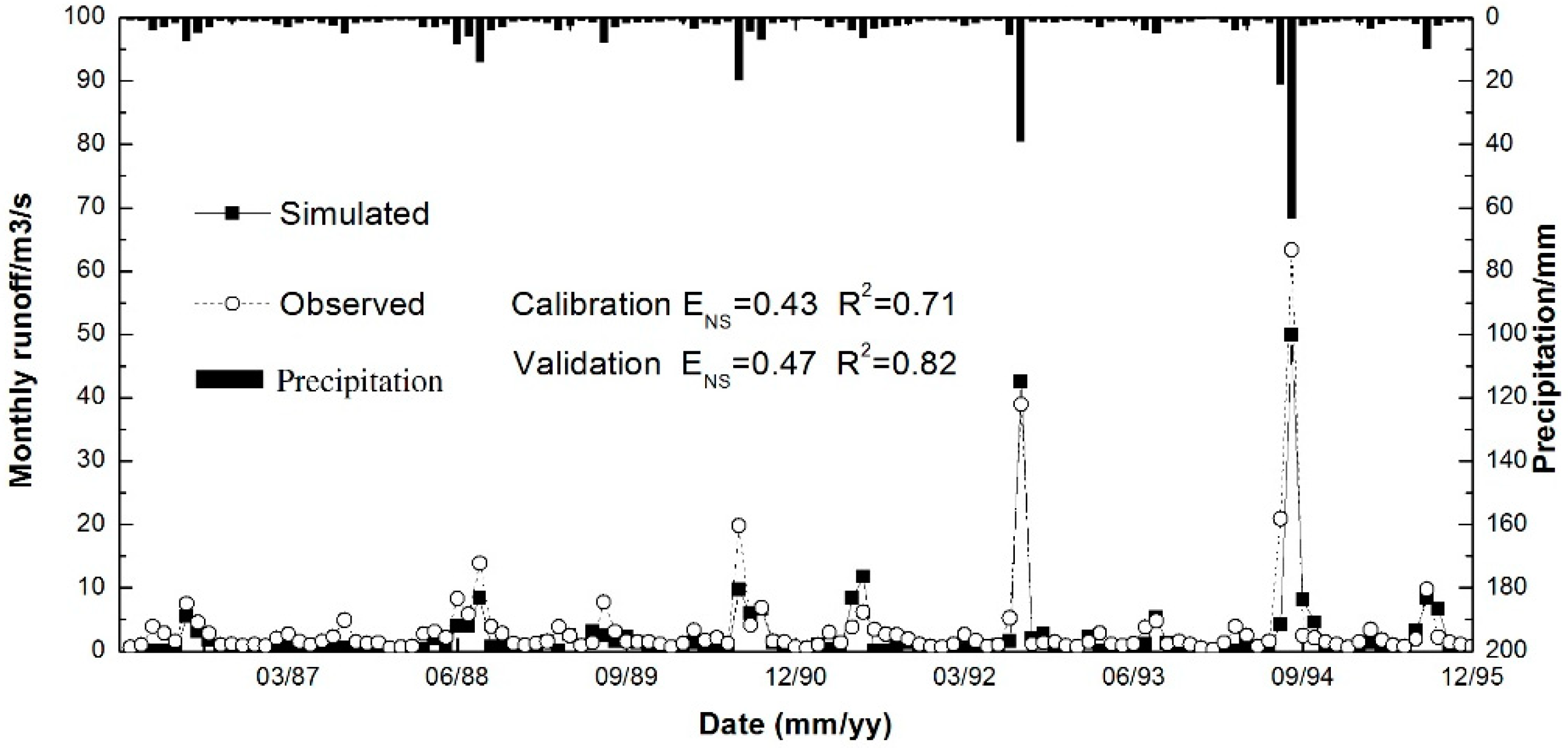
After the sensitive parameter analysis, the model was calibrated for the observed values in 1986–1990 and validated for 1991–1995. The Nash–Sutcliffe efficiency (E_NS) and the regression coefficient (R²) were used to evaluate the fitness of SWAT between the simulated and observed values. The variation range of E_NS was from negative infinity to 1. Model performance increased with higher R².

Table 3. Model performance for the simulation of runoff yields.

Period	Monthly		Year
	ENS	R2	ENS	R2
Calibration (1986–1990)	0.43	0.71	0.66	0.76
Validation (1991–1995)	0.47	0.82	0.72	0.89

shows that the model was acceptable for the calibrated and validated periods. The observed and simulated average annual runoff depths during the calibration period were 26.2 and 21.7 mm, respectively. For the 1991–1995 validation period, the observed and simulated average annual runoff depths were 38.3 and 36.5 mm, respectively. Figure 3 and Figure 4 suggested that there was good agreement between the observed and simulated results at both monthly and yearly scales, while the results also indicated that the model underestimated runoff. Although the model-simulated runoff at the monthly scale was not as good as that at the annual scale, its performance was still acceptable according to the criteria given by Moriasi et al. (2007). Overall, the calibrated model was reliable and acceptable for the simulation of runoff for further analysis during the changed period of hydrological processes.

In this research, three scenarios including only LULC change, only climate change, and combined climate and LULC change were established to predict the individual and combined impacts on water balance. Water balance in the catchment from 2020–2050 was simulated in correspondence with each scenario within the three periods including the 2020s, 2030s, and 2040s. The simulated water balance for the future period under each scenario was compared with the baseline value (2002–2012). To analyze the impact of climate change on the water balance, Scenario 1 was simulated, and land use was assumed to be same as in 2010. To analyze the impact of LULC changes on the water balance, Scenario 2 was simulated with the LULC in 2025, 2035, and 2045. The future climate was assumed to be consistent with that in the baseline period. Scenario 3 was constructed to analyze the effects of climate and LULC changes on future water balance.

4.2. CA-Markov Chain-Based Land Use Change Prediction

The land use classification of 1995 and 2010 TM images was interpreted through the adoption of the maximum likelihood classification (MLC). In this study area, land uses were divided into five sectors: agriculture, grassland, forest, urban, and water. As shown in

Table 4. Land use area statistics of 1995, 2000, and 2010.

Land Use	1995		2000		2010
	Area (km2)	Area (%)	Area (km2)	Area (%)	Area (km2)	Area (%)
Agriculture	1594.75	46.79	1454.88	42.69	497.25	14.59
Grassland	1701.92	49.94	1847.14	54.20	2161.6	63.43
Forest	95.32	2.8	100.2	2.94	714.12	20.95
Water	12.14	0.36	3.07	0.09	17.76	0.52
Settlement	3.87	0.11	2.83	0.08	17.26	0.51

and Figure 5, agricultural land and grassland occupied the highest percentage of the total area in 1995: 46.8 and 49.9%, respectively. In 2000, the dominant land use types were still agriculture and grassland, although the agricultural area decreased by 4.1%. Until 2010, the land use structure underwent fundamental changes. Grassland and forest were the dominant land use types in the catchment, the percentages of which were 63.4 and 20.9%, respectively. These percentage changes to land use area indicated that the vegetation coverage gradually increased under the “Grain to Green” program on the Loess Plateau of China. Yan et al. (2016) [25] employed Landsat TM image data and found that the average vegetation coverage increased from 19.2 to 38.8% from 1995 to 2014, consistent with the presentation in Table 4.

The future land use changes in 2025, 2035, and 2045 were predicted through the CA-Markov model within the IDRISI software. In this study area, the transfer area matrix and transfer probability matrix were identified according to the land use data from 1995 to 2010. Suitability images of different land use types were established by the multi-criteria evaluation (MCE). The matrix introduces the possibility of reverting from one class to every other class [35]. The CA-model predicted that, in the 2010–2025 changes shown in

Table 5. Land use area statistics of 2025, 2035, and 2045.

Land Use	2025		2035		2045
	Area (km2)	Area (%)	Area (km2)	Area (%)	Area (km2)	Area (%)
Agriculture	380.37	11.16	356.71	10.47	306.17	8.98
Grassland	1984.13	58.22	1996.76	58.59	2022.99	59.36
Forest	960.07	28.17	971.06	28.49	995.20	29.20
Water	36.43	1.07	36.47	1.07	36.62	1.07
Settlement	47.00	1.38	47.00	1.38	47.01	1.38

and Figure 5, agricultural land and grassland will convert mostly to forest in the watershed, with additional areas of 116.8 and 177.5 km², respectively, which might be possible due to a continuous soil and water conservation project in the future. Settlement and water areas will also increase by 29.7 and 18.7 km², respectively. In the 2025 to 2035 changes, agricultural land was continuously predicted to slightly convert to forest in the watershed, with an additional area of 23.66 km², and grassland to increase by 12.63 km², compared to 2025. The settlement and water areas were more stable than the other land use types.

The smallest changes were observed in the 2035–2045 transitional period. There was a transformation pattern similar to that of the 2025–2035 changes. Agricultural land was slightly converted to forest and grassland, with an additional area of 50.54 km². Changes to grassland and forest were very low, slightly increasing by 26.2 and 24.1 km², respectively. In this period, water and settlement areas remained stable. Hence, under this change trend, increasing forests may lead to increasing demands on soil water for vegetation restoration on the semi-arid loess plateau [36,37].

4.3. Investigating Future Climate Change through the CLIGEN Model

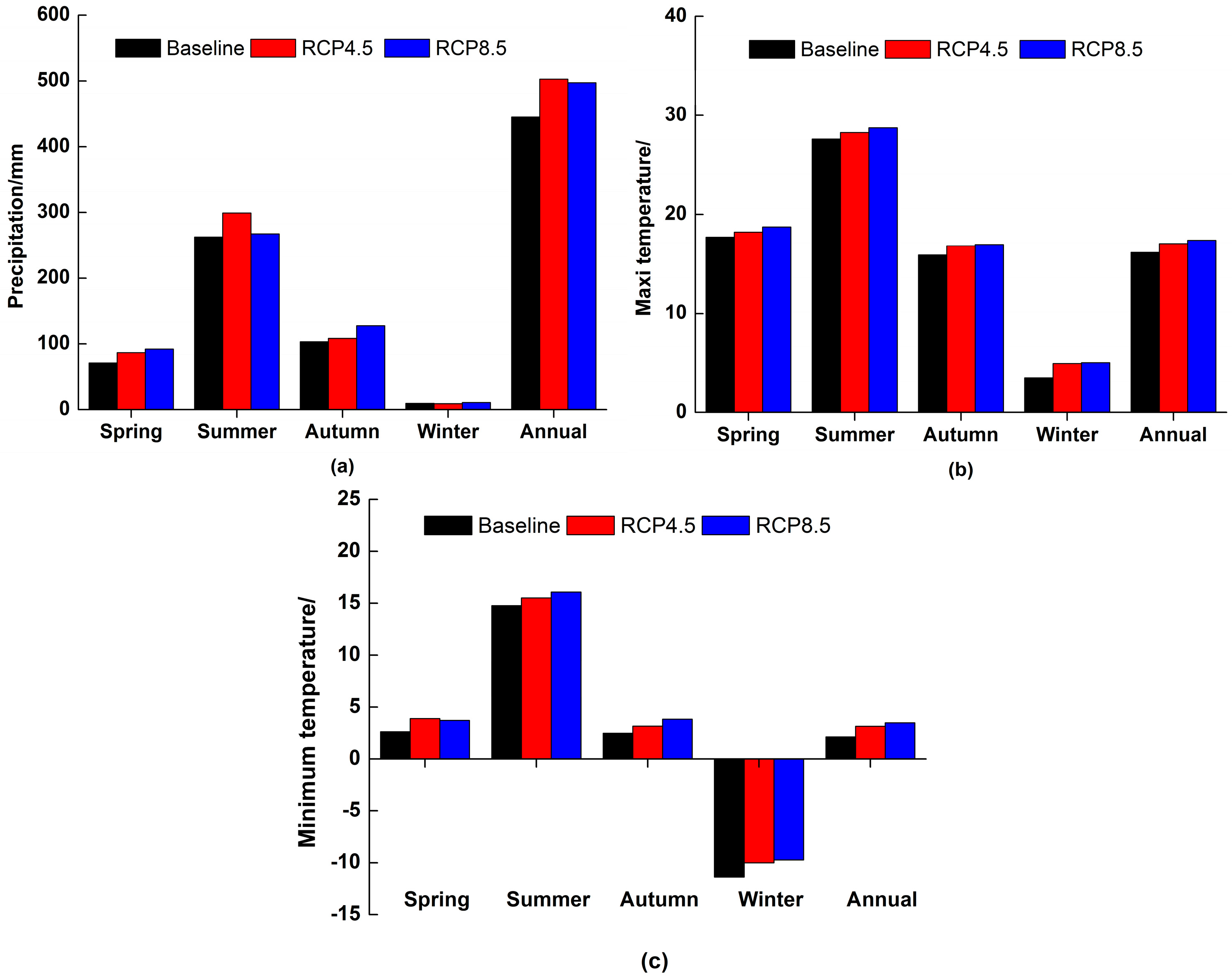
Historical and future changes in annual precipitation and temperature derived for RCP4.5 and RCP8.5 are presented in Figure 6. The results showed that, for both RCP4.5 and RCP8.5, the precipitation from 2020 to 2050 in the study area annually and in different seasons was higher than the historical values. As shown in Figure 6, at an annual scale, the precipitation in RCP4.5 and RCP8.5 increased by 57.4 and 52.1 mm compared with the baseline period. The precipitation in all seasons under RCP8.5 was higher than under RCP4.5, except in summer. Similarly, the maximum and minimum temperatures were higher than for the baseline period in both the RCP4.5 and RCP8.5 scenarios, and the maximum and minimum temperatures in RCP8.5 were 0.31 and 0.33 °C higher, respectively, than those in RCP4.5. The increased temperatures were larger in winter than in other seasons in the future, and the maximum temperatures increased by 1.5 and 1.6 °C for RCP4.5 and RCP8.5, respectively. Similarly, the minimum temperatures increased by 1.36 and 1.64 °C in the two scenarios. The estimations indicate an overall warming of the study area, with higher temperatures for both the RCP4.5 and RCP8.5 scenarios. However, these future climate changes might be due to the risks of drought or water quantity in the basin.

4.4. Sensitivity Analysis of Runoff to Climate and Land Use Change

To evaluate the sensitivity of runoff to climate, six climate scenarios were established that included 5, 10 and 20% increases in precipitation and 0.5, 1, and 2 °C increases in maximum and minimum temperatures. These climate scenarios were then incorporated into the SWAT model with the same land use map in 2010. The results (

Table 6. Climate elasticity coefficient for different scenarios.

Scenarios	+5%	+10%	+20%	Scenarios	+0.5 °C	+1 °C	+2 °C
Precipitation	3.30	4.40	5.93	Maximum temperature	0.24	0.26	0.25
—	—	—	—	Minimum temperature	0.15	0.16	0.16

) showed that runoff was most sensitive to rainfall changes, followed by the maximum and minimum temperatures. The research also found that the greater the increase in rainfall, the greater the sensitivity of runoff to rainfall. However, the temperature sensitivity remained stable.

Five potential land use scenarios were developed to analyze the sensitivity of runoff to different land use types: (1) forest and pasture were converted to agriculture, and the rest remained unchanged; (2) agriculture and forest were converted to pasture, and the rest remained unchanged; (3) agriculture and pasture were converted to forest, and the rest remained unchanged; (4) settlement was converted to pasture, and the rest remained unchanged; and (5) water was converted to pasture, and the rest remained unchanged. The thus derived land use scenarios were incorporated into the SWAT model for determination of new HRUs for each sub-basin, and a series of parameters remained stable. Next, simulation results combined with the formula for calculating the elasticity coefficient were used to calculate the runoff response coefficient. The research (

Table 7. Runoff response coefficient under the extreme land use scenario.

Land Use Type	Agriculture	Forest	Grassland	Water	Settlement
Runoff response coefficient	0.86	0.35	0.40	2.21	3.36

) found that there were different runoff response coefficients for different underlying surface coverage types. The runoff sensitivity coefficients in decreasing order were for settlement, water, agricultural land, grassland, and forest, the corresponding values of which were 3.36, 2.23, 0.86, 0.39, and 0.34. Settlement had the highest degree of sensitivity to runoff, but the sensitivity of runoff to forest was the lowest. In general, runoff was more sensitive to rainfall than to land use change in this watershed. Therefore, the increase in rainfall more easily causes flooding and soil erosion in the basin.

4.5. Water Balance Analysis

There were three conditions to be considered in this analysis: (a) the individual impact of land use changes on water balance, (b) the individual impact of climate change on water balance, and (c) the combined impacts of both on water balance.

4.5.1. Impacts of Land Use Changes

The dominant land use types of the watershed were agriculture, grassland, and forest. Therefore, to evaluate the impacts of land use change on water balance, the calibrated SWAT model was simulated in three future land use scenarios in 2025, 2035, and 2045 under the assumption that the weather did not change. The results are given in

Table 8. Water balance due to future land use change.

Year	P	Runoff		ET		Water Yield
	mm	mm	%	mm	%	mm	%
2010	460.09	13.57	–	408.49	–	37.04	–
2025	460.09	13.16	−3.02	440.35	7.80	31.89	−13.90
2035	460.09	13.06	−3.76	442.06	8.22	30.72	−17.06
2045	460.09	12.95	−4.57	443.12	8.48	29.52	−20.30

, and show that runoff may decline in the future under the change in land use, decreasing by 3.02, 3.76, and 4.57% for land use in 2025, 2035, and 2045, respectively, when compared with land use in 2010. Similarly, water yield also gradually decreased in the simulation by 13.9, 17.06, and 20.3% for 2025, 2035, and 2045, respectively. Oppositely, evapotranspiration gradually increased by 7.80, 8.22, and 8.48% in comparison with that in 2010. This can be attributed to a trend in agriculture transformation to grassland and forest in the future.

Crops with shallow-root systems have less water storage capacity than forests and grasses, and under the future land use change in the watershed, the runoff and water yield would ultimately decrease. Table 6 also shows the relative changes in the annual water balance for the future land uses in 2025, 2035, and 2045. In addition, it has been widely researched that increased vegetation coverage is usually associated with decreased flow [38].

4.5.2. Impacts of Climate Change

To understand hydrological processes, including precipitation, runoff, ET (evapotranspiration), and water yield in the watershed, the calibrated SWAT model was simulated using the RCP4.5 and RCP8.5 future precipitation and temperature data scenarios, respectively. The simulated water balances for future periods under scenarios RCP4.5 and RCP8.5 were compared to the corresponding values in the baseline period (2002–2012). Table 7 shows the seasonal and annual changes under the climate scenarios for the 2020–2050 period. Runoff and water yield increased by 29.0–83.9% and by 11.4–37.7%, respectively, in both scenarios on an annual scale (Figure 7). Similarly, ET also gradually increased by 4.3–14.6% from 2020 to 2050. The reason may be that rising temperature leads to an increase in ET.

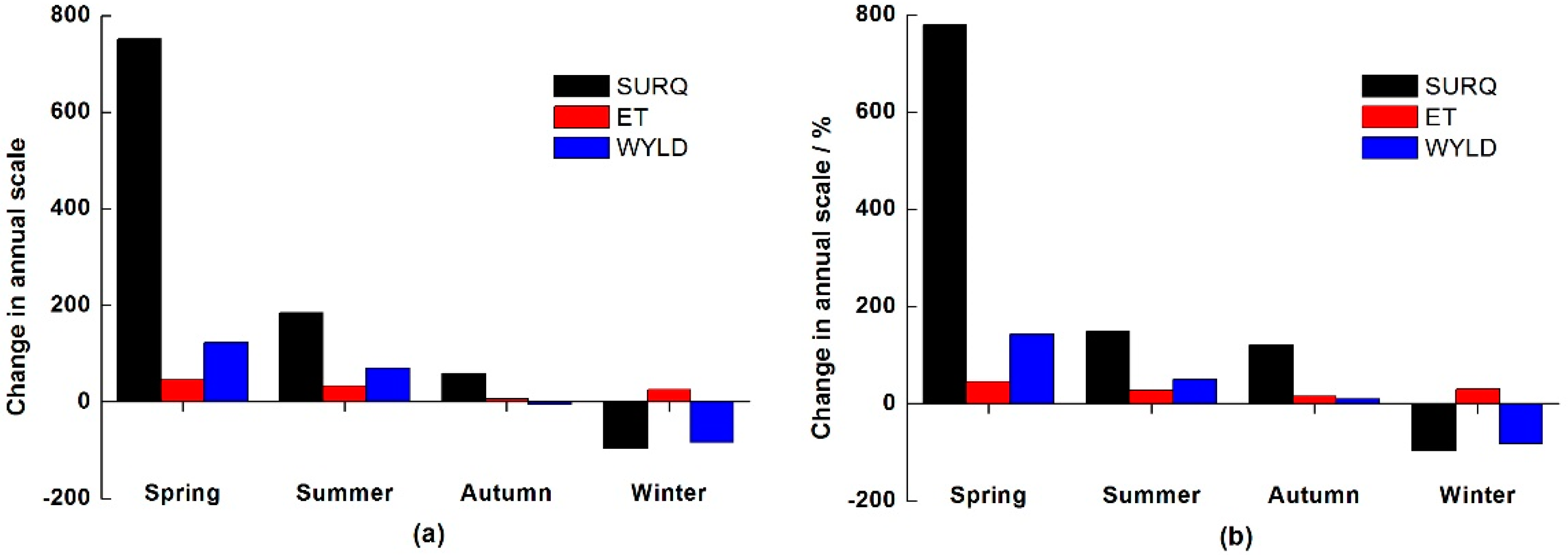
On a seasonal scale, water balance including runoff, water yield, and ET gradually increased in spring, summer, and autumn and decreased in winter (Figure 8 and

Table 9. Seasonal and annual changes in water balance during the baseline period (2002–2012) and future period (2020–2050) for RCP4.5 and RCP8.5 scenarios.

Variables	Periods		Spring	Summer	Autumn	Winter	Annual
Runoff	Baseline period	2002–2012	0.83	6.85	2.46	1.52	11.65
	RCP4.5	2020–2029	3.07	13.19	1.41	0.10	17.76
		2030–2039	2.36	11.88	6.22	0.03	20.49
		2040–2050	1.30	16.20	1.91	0.04	19.46
	RCP8.5	2020–2029	2.18	12.08	7.05	0.12	21.42
		2030–2039	2.28	14.87	2.82	0.07	20.04
		2040–2050	2.53	9.09	3.37	0.05	15.03
Water yield	Baseline period	2002–2012	3.18	19.07	10.62	1.77	34.64
	RCP4.5	2020–2029	6.21	27.90	7.89	0.33	42.33
		2030–2039	5.99	27.57	13.66	0.49	47.71
		2040–2050	4.94	30.97	7.42	0.29	43.62
	RCP8.5	2020–2029	6.47	25.78	13.86	0.42	46.52
		2030–2039	5.71	28.57	9.76	0.42	44.45
		2040–2050	6.51	21.86	9.85	0.38	38.59
ET	Baseline period	2002–2012	81.19	201.50	103.76	19.31	405.76
	RCP4.5	2020–2029	81.81	230.26	102.80	16.14	431.01
		2030–2039	99.94	248.82	98.01	18.12	464.89
		2040–2050	98.18	227.58	86.34	15.79	427.88
	RCP8.5	2020–2029	92.35	228.67	105.32	17.15	443.49
		2030–2039	89.95	227.56	112.32	17.49	447.31
		2040–2050	95.71	213.77	96.41	17.50	423.40

). The results indicate that there were some differences between the scenarios; briefly, runoff and water yield were simulated for the future period of 2020 to 2050 and were found to decrease in winter but increase in spring, summer, and autumn. In particular, runoff increased by 73.4–136.5% under RCP4.5 in summer and by 32.7–117.1% under RCP8.5. In winter, runoff gradually decreased by 93.4–98.0% and by 92.1–96.7% for RCP4.5 and RCP8.5, respectively. Seasonal changes indicated that the runoff and water yield increased under both RCP4.5 and RCP8.5 in spring and summer. Runoff and water yield gradually decreased in the future, although the precipitation increased at the same time. Those results indicated that water balance in this study area was impacted not only by precipitation but was also sensitive to the change in temperature.

Figure 7 also shows the relative changes in the annual water balance in the 2020s, 2030s, and 2040s as box-and-whisker plots. In the 2020s, 2030s, and 2040s, the ranges of relative changes in runoff were larger than the annual water yield and ET. In addition, the sensitivity of water balance to climate change differed in different seasons. In addition, the runoff and water yield were more susceptible to the climate change in spring and winter seasons than in summer and autumn seasons. Although the runoff and water yield in dry seasons accounted for a small portion of the annual value, it was related to the low flow in the watershed. The amount of low flow also influences the ecosystem health and spring flood. Because of the dwindling vegetation coverage in spring, the probability of occurrence of soil and water erosion would be relatively large if the precipitation were to increase in the future. Hence, it is crucial to understand the influence of climate change in low flow and drought situations in spring [39].

4.5.3. Combined Impacts of Climate and LULC Changes

The combined impacts of future land use changes and climate variability on water balance in the study area were simulated with the calibrated SWAT model, the results of which are presented in Figure 9 and Figure 10. The variation in the relative changes of runoff was larger than for both water yield and ET in all the scenarios. In comparison with the baseline period, the runoff gradually increased in the future in general, although it dropped a little during a certain period of time. Water yield and ET also gradually increased compared with those in the baseline period.

As shown in Figure 10, runoff increased in spring, summer, and autumn and decreased in winter from 2020 to 2050. The relative changes, which ranged from 387.1 to 502.5%, were larger in spring than those in other seasons. The reason may be that runoff change was more susceptible in spring than in other seasons. ET increased in summer and winter but decreased in spring, except for the LULC2045 & RCP8.5 scenario. In autumn, ET decreased in the RCP4.5 scenario but increased under RCP8.5. This factor might be that the average precipitation under RCP4.5 was lower than under RCP8.5 from 2020 to 2050. Similarly, water yield increased in spring and summer and declined in autumn in the RCP4.5 scenario. The ranges of relative change were 95.4–281.2% in spring and 26.2–191.2% in summer. In winter, water yield decreased, and the range of variations was from −23.8 to −254.9%. We also found that the ranges of relative changes in runoff were larger than for water yield and ET.

Generally, the variation trend from the simulation of land use and climate changes was similar to the results for the simulation of climate change taken alone. The reason might be that, according to the combined effects of future land use change and climate variability, the decrease in runoff magnitude caused by future land use change might be offset by climate change, and the relative changes in runoff for the future climate variability were larger than for the future land use change. Runoff was more sensitive to climate variability than to land use change, and the relative changes for the future scenarios of climate and land use changes were obviously consistent with the scenario of future climate change alone. It was useful to understand the changes in water balance affected by the separate and coupled impacts of potential climate and land use changes for water management and sustainable water resource policy. The change in distributed runoff in different seasons and extreme weather events inevitably aroused the flooding and droughts for the forthcoming period in the watershed. More flexible and adaptable soil and water conservation measures should be established to confront the probable impacts. In general, these findings could contribute to effective local government risk management policies according to the potential for floods and droughts in the watershed.

5. Conclusions

This study investigated the individual and combined impacts of future LULC and climate changes on water balance in the upper reaches of the Beiluo River basin on the Loess Plateau of China. Three scenarios were established and estimated by the SWAT model. In addition, the future water balance was compared with those of the baseline period. Agriculture areas decreased by 32.2% from 1995 to 2010, while increases in forest and grassland areas of 13.49 and 18.15%, respectively, were indicated from 1995 to 2010. Predictions of LULC were simulated by the CA-Markov model. The land use predictions of 2025, 2035, and 2045 indicated rising forest areas with decreased agricultural land and grassland. Although grassland increased from 2025 to 2045, grassland areas decreased compared with LULC in 2010. Water and settlement areas increased by 0.55 and 0.87% from 2010 to 2025, respectively, and their areas remained stable from 2025 to 2045. Climate data simulated by a regional climate model (RegCM4.0) under RCP4.5 and RCP8.5 were obtained for the future climate analysis. The SWAT model was calibrated and validated by calculating the historical runoff over the period 1986–1995. The agreement between observed and simulated monthly runoff values indicated that, after the parameters were optimized, the calibrated model could be used to simulate the responses of water balance to climate and LULC changes in this study area.

The past and future impacts of the scenarios were simulated under the seasonal and annual scales of water balance. Future runoff, water yield, and ET increased at an annual scale under both scenarios. Increased rainfall and temperature in the future lead to increased runoff, water yield, and ET in spring, summer, and autumn and decreased runoff, water yield, and ET in winter from 2020 to 2050. LULC change had a smaller impact on the water balance than did climate change. On an annual scale, runoff and water yield gradually decreased in the future, but ET increased. The combined effects of both LULC and climate changes on water balance in the future were similar to the variation trend of climate changes alone at both annual and seasonal scales. Researching the effects of the individual and combined LULC and climate changes on water balance is important for rational water resource planning and management. The study area is located in the semi-arid Loess Plateau in China, and increasing forest areas may increase the demands of soil water requirements. The seasonal change in water balance in this study area is likely to be more severe in the future. Runoff increases in summer might lead to increasing extreme weather events and flood frequency.

Future water resource plans should adopt a long-term perspective, adapt to insights, and consider these impacts. In addition, governments should work together and develop sustainable land use plans to maintain a balance with ecological water requirements. The results of this research can be helpful for effective planning aimed at flood and drought management and prevention.

References

- Brath, A.; Montanari, A.; Moretti, G. Assessing the effect on flood frequency of land use change via hydrological simulation (with uncertainty). J. Hydrol. 2006, 324, 141–153. [Google Scholar] [CrossRef]
- Chien, H.; Yeh, P.J.F.; Knouft, J.H. Modeling the potential impacts of climate change on streamflow in agricultural watersheds of the Midwestern United States. J. Hydrol. 2013, 491, 73–88. [Google Scholar] [CrossRef]
- Mendes, J.; Maia, R. Hydrologic Modelling Calibration for Operational Flood Forecasting. Water Resour. Manag. 2016, 30, 5671–5685. [Google Scholar] [CrossRef]
- Li, Z.; Liu, W.Z.; Zhang, X.C.; Zheng, F.L. Impacts of land use change and climate variability on hydrology in an agricultural catchment on the Loess Plateau of China. J. Hydrol. 2009, 377, 35–42. [Google Scholar] [CrossRef]
- Costa, M.H.; Botta, A.; Cardille, J.A. Effects of large-scale changes in land cover on the discharge of the Tocantins River, Southeastern Amazonia. J. Hydrol. 2003, 283, 206–217. [Google Scholar] [CrossRef]
- Zuo, D.P.; Xu, Z.X.; Yao, W.Y.; Jin, S.Y.; Xiao, P.Q.; Ran, D.C. Assessing the effect of changes in land use and climate on runoff and sediment yields from a watershed in the Loess Plateau of China. Sci. Total Environ. 2016, 544, 238–250. [Google Scholar] [CrossRef] [PubMed]
- Asl-Rousta, B.; Mousavi, S.J.; Ehtiat, M. SWAT-Based Hydrological Modelling Using Model Selection Criteria. Water Resour. Manag. 2018, 32, 2181–2197. [Google Scholar] [CrossRef]
- Brown, A.; Zhang, L.; McMahon, T.; Western, A.; Vertessy, R. A review of paired catchment studies with reference to the seasonal flows. J. Hydrol. 2005, 310, 28–61. [Google Scholar] [CrossRef]
- Germer, S.; Neill, C.; Vetter, T.; Chaves, J.; Krusche, A.V.; Elsenbeer, H. Implications of long-term land-use change for the hydrology and solute budgets of small catchments in Amazonia. J. Hydrol. 2009, 364, 349–363. [Google Scholar] [CrossRef]
- Qi, J.Y.; Li, S.; Yang, Q.; Xing, Z.S.; Meng, F.R. SWAT Setup with Long-Term Detailed Landuse and Management Records and Modification for a Micro-Watershed Influenced by Freeze-Thaw Cycles. Water Resour. Manag. 2017, 31, 3953–3974. [Google Scholar] [CrossRef]
- Dias, L.C.P.; Macedo, M.N.; Costa, M.H.; Coe, M.T.; Neill, C. Effects of land cover change on evapotranspiration and streamflow of small catchments in the Upper Xingu River Basin, Central Brazil. J. Hydrol. Reg. Stud. 2015, 4, 108–122. [Google Scholar] [CrossRef] [Green Version]
- Lamparter, G.; Nobrega, R.; Kovacs, K.; Amorim, R.S.; Gerold, G. Modelling hydrological impacts of agricultural expansion in two macro catchments in Southern Amazonia, Brazil. Reg. Environ. Chang. 2018, 18, 91103. [Google Scholar] [CrossRef]
- Zhang, J.J.; Zhang, X.P.; Li, R.; Chen, L.L.; Lin, P.F. Did streamflow or suspended sediment concentration changes reduce sediment load in the middle reaches of the Yellow River? J. Hydrol. 2017, 546, 357–369. [Google Scholar] [CrossRef]
- Liu, E.J.; Zhang, X.P.; Xie, M.L. Hydrologic responses to vegetation restoration and their 584 driving forces in a catchment in the Loess hilly-gully area: A case study in the upper Beiluo 585 River. Acta Ecol. Sin. 2015, 35, 623–629. (In Chinese) [Google Scholar]
- Chen, N.; Ma, T.Y.; Zhang, X.P. Response of soil erosion processes to land cover changes 535 in the Loess Plateau of China: A case study on the Beiluo River basin. Catena 2016, 136, 118–127. [Google Scholar] [CrossRef]
- Yan, R.; Zhang, X.P.; Yan, S.J.; Zhang, J.J.; Chen, H. Spatial patterns of hydrological responses to land use/cover change in a catchment on the Loess Plateau, China. Ecol. Indic. 2017. [Google Scholar] [CrossRef]
- Li, Z.; Liu, W.Z.; Zheng, F.L. Land use change in Heihe catchment on loess tableland based on CA-Markov model. Trans. CSAE 2010, 26, 346–352. (In Chinese) [Google Scholar]
- Li, Z.; Jin, J.M. Evaluating climate change impacts on streamflow variability based on a multisite multivariate GCM downscaling method in the Jing River of China. Hydrol. Earth Syst. 2017, 21, 5531–5546. [Google Scholar] [CrossRef] [Green Version]
- Ficklin, D.L.; Luo, Y.; Luedeling, E.; Zhang, M. Climate change sensitivity assessment of a highly agricultural watershed using SWAT. J. Hydrol. 2009, 374, 16–29. [Google Scholar] [CrossRef]
- Moradkhani, H.; Baird, R.G.; Wherry, S.A. Assessment of climate change impact on floodplain and hydrologic ecotones. J. Hydrol. 2010, 395, 264–278. [Google Scholar] [CrossRef]
- Praskievicz, S.; Chang, H. Impacts of climate change and urban development on water resources in the Tualatin River Basin, Oregon. Ann. Assoc. Am. Geogr. 2011, 101, 249–271. [Google Scholar] [CrossRef]
- Yoshimura, C.; Zhou, M.; Kiem, A.S.; Fukami, K.; Prasantha, H.H.; Ishidaira, H. 2020s scenario analysis of nutrient load in the Mekong River Basin using a distributed hydrological model. Sci. Total Environ. 2009, 407, 5356–5366. [Google Scholar] [CrossRef] [PubMed]
- Moss, R.H.; Edmonds, J.A.; Hibbard, K.A.; Manning, M.R.; Rose, S.K.; Van, D.P. The next generation of scenarios for climate change research and assessment. Nature 2010, 463, 747–756. [Google Scholar] [CrossRef] [PubMed]
- Riahi, K.; Rao, S.; Krey, V.; Cho, C.; Chirkov, V.; Fischer, G. RCP 8.5-a scenario of comparatively high greenhouse gas emissions. Clim. Chang. 2011, 109, 33–57. [Google Scholar] [CrossRef]
- Yan, R.; Zhang, X.P.; Yan, S.J.; Zhao, W.H. The vegetation restoration in the Beiluo River Basin from 1995 to 2014 and their distribution on the landform. J. Northeast. Univ. (Nat. Sci.) 2016, 37, 1598–1603. (In Chinese) [Google Scholar]
- Zhang, X.P.; Zhang, L.; Zhao, J.; Rustomji, P.; Hairsine, P. Responses of streamflow to changes in climate and land use/cover in the Loess Plateau, China. Water Resour. Res. 2008, 44, W00A07. [Google Scholar] [CrossRef]
- Hou, X.Y.; Chang, B.; Yu, X.F. Land use change in Hexi corridor based on CA–Markov methods. Trans. CSAE 2004, 20, 286–291. (In Chinese) [Google Scholar]
- Giorgi, F.; Coppola, E.; Solmon, F.; Mariotti, L.; Sylla, M.B.; Bi, X.; Elguindi, N.; Diro, G.T.; Nair, V.; Giuliani, G.; et al. RegCM4: Model description and preliminary tests over multiple CORDEX domains. Clim. Res. 2012, 52, 7–29. [Google Scholar] [CrossRef]
- Zhang, X.C.; Garbrecht, J.D. Evaluation of CLIGEN precipitation parameters and their implication on WEPP runoff and erosion prediction. Trans. ASAE 2003, 46, 311–320. [Google Scholar] [CrossRef]
- Breuer, L.; Huisman, J.; Willems, P.; Bormann, H.; Bronstert, A.; Croke, B.; Frede, H.G.; Graff, H.T.; Jakeman, L. Assessing the impact of land use change on hydrology by ensemble modeling (LUCHEM). I: Model intercomparison with current land use. Adv. Water Resour. 2009, 32, 129–146. [Google Scholar] [CrossRef]
- Nash, J.E.; Sutcliffe, J.V. River flow forecasting through conceptual models part I—A 604 discussion of principles. J. Hydrol. 1970, 10, 282–290. [Google Scholar] [CrossRef]
- Moriasi, D.N.; Arnold, J.G.; Bingner, R.L.; Harmel, R.D.; Veith, T.L. Model evaluation guidelines for systematic quantification of accuracy in watershed simulations. Trans ASABE 2007, 50, 885–900. [Google Scholar] [CrossRef]
- Legesse, D.; Vallet-Coulomb, C.; Gasse, F. Hydrological response of a catchment to climate and land use changes in Tropical Africa: Case study South Central Ethiopia. J. Hydrol. 2003, 275, 67–85. [Google Scholar] [CrossRef]
- Gao, G.Y.; Fu, B.J.; Wang, S.; Liang, W.; Jiang, X.H. Determining the hydrological responses to climate variability and land use/cover change in the Loess Plateau with the Budyko framework. Sci. Total Environ. 2016, 557, 331–342. [Google Scholar] [CrossRef] [PubMed] [Green Version]
- Sang, L.L.; Zhang, C.; Yang, J.Y.; Zhu, D.H.; Yun, W.J. Simulation of land use spatial pattern of towns and villages based on CA-Markov model. Math. Comput. Model. 2012, 54, 938–943. [Google Scholar] [CrossRef]
- Li, S.; Wei, L.; Fu, B.J. Vegetation changes in recent large-scale ecological restoration projects and subsequent impact on water resources in China’s Loess Plateau. Sci. Total Environ. 2016, 569, 1032–1039. [Google Scholar] [CrossRef]
- Yang, Y.G.; Fu, B.J. Soil water migration in the unsaturated zone of semiarid region in China from isotope evidence. Hydrol. Earth Syst. Sci. 2017, 21, 1757–1767. [Google Scholar] [CrossRef] [Green Version]
- White, M.D.; Greer, K.A. The effects of watershed urbanization on the stream hydrology and riparian vegetation of Los Peñasquitos Creek, California. Landsc. Urban Plan. 2006, 74, 125–138. [Google Scholar] [CrossRef]
- Bae, D.H.; Jung, I.W.; Lettenmaier, D.P. Hydrologic uncertainties in climate change from IPCC AR4 GCM simulations of the Chungju Basin, Korea. J. Hydrol. 2011, 401, 90–105. [Google Scholar] [CrossRef]
Figure 1.
Locations of the upper reaches of the Beiluo River basin (c) and the Loess Plateau (b) in China (a).
Figure 2.
Methodology.
Figure 3.
Observed and simulated annual runoff depths for the study catchment.
Figure 4.
Observed and simulated average monthly runoff for the study catchment.
Figure 5.
Land use maps of 1995, 2000, 2010, 2025, 2035, and 2045.
Figure 6.
Meteorological data measured in the catchment at the weather station (1969–2012) and projected under the RCP4.5 and 8.5 scenarios. Mean seasonal and annual (a) precipitation. (b) Maximum temperature. (c) Minimum temperature.
Figure 7.
Box-and-whisker plots showing changes in annual runoff (SURQ), water yield (WYLD), and evapotranspiration (ET): (a) 2020s, (b) 2030s, and (c) 2040s.
Figure 8.
Changes in seasonal SURQ, ET, and WYLD relative to the baseline period under the RCP4.5 (a) and RCP8.5 (b) scenarios.
Figure 9.
Box-and-whisker plots showing changes in seasonal and annual SURQ, ET, and WYLD under Scenario 3 for the future period relative to the baseline period.
Figure 10.
Changes in seasonal: (a) SURQ, (b) ET, and (c) WYLD under Scenario 3 for the future period relative to the baseline period.