Designing Optimum Water-Saving Policy in China Using Quantity and Price Control Mechanisms

Abstract

In an attempt to alleviate water scarcity, the government of China has introduced a water plan for the year 2030. Based on a dynamic computable general equilibrium model, this paper investigates how conservation of irrigation water, grain production, and the welfare of rural households will be affected by planned reductions to the irrigation water subsidy between 2018 and 2030. Four policy instruments, namely quantitative control (QC), quantitative control with a subsidy reduction (QC-SR), price control (PC), and price control with a subsidy reduction (PC-SR) are employed in the model. Most existing research has found that reducing the irrigation subsidy will lead to significant negative impacts to the agricultural economy, and especially to rural households. These predicted negative impacts are a barrier to agricultural water policy pricing reform. However, the results of this research show that a provincial subsidy reduction to 1% between 2018 and 2030 will have an insignificant impact on agricultural production as well as rural household incomes and welfare, despite the subsidy rate currently accounting for more than 90% of the total irrigation value at the macro level in most provinces. Furthermore, PC will create a demand for irrigation water, which is predicted to rise to more than five times the agricultural water planning level currently set for 2030, and PC-SR will not achieve the agricultural water planning goal.

1. Introduction

Water scarcity is one of the greatest environmental challenges facing the world today and, in many places, reliable water services can no longer be guaranteed. According to the World Economic Forum, by 2030, global water demand will outstrip supply by 40% [1]. In September 2016, the Member States of the United Nations adopted the 2030 agenda for Sustainable Development with 17 Sustainable Development Goals (SDGs). SDG 6 sought to “ensure availability and sustainable management of water and sanitation for all”. One of the targets within SDG 6 is addressing water scarcity by ensuring sustainable withdrawals and supply of freshwater by 2030 [2]. Moreover, the United Nations General Assembly has declared 2018-2028 the International Water Action Decade, where efforts will be accelerated to focus on “the sustainable development and integrated management of water resources for the achievement of social, economic, and environmental objectives” [3]. Globally, agriculture accounts for 60% to 90% of fresh water consumption [4] and, due to population growth and changing dietary habits, agricultural demands for water are increasing. The FAO estimates that, by 2050, 60% more food will need to be produced to satisfy a growing global population, which will require greater quantities of water for irrigation [4]. This increased demand for irrigation water will coincide with increased incidence of climate change induced drought, which further exacerbates water scarcity [5].

Despite being home to 20% of the world’s population, China contains only 7% of global freshwater resources and 80% of this water is concentrated in the south of the country [6]. Across China, agriculture accounts for more than 60% of total water use. With increasing water demand from rapidly growing industries and urban populations, water scarcity is already a major stress factor in agricultural production [7,8]. Improving water resource management is a long-term goal of the Chinese government. According to Yong [9], this requires a holistic approach that incorporates institution-building, market-based approaches and capacity-building. Efforts to alleviate water scarcity are divided between supply enhancement and demand management [4]. The former requires technological advancement, while the latter, which is the subject of this paper, is achieved through both quantitative control (QC) and price control (PC).

A large body of scholarly literature provides the theoretical basis and practical evidence to support these water demand management methods. An example of quantitative control is the imposition of water quotas, as a mechanism to curtail water demand. The quota method, however, lacks flexibility to respond to changing circumstances, such as those experienced by farmers. Price control is an economic tool used to promote efficient water use and conservation. This market model received international approval at the UN’s 1992 conference on Water and Sustainable Development [10]. It can benefit agricultural production through lower pricing of irrigation water. However, research suggests that this is a primary cause of excessive water use [11].

In the long term, quantitative control follows annual quantitative planning. In the short term, price control protects farmers’ incentives to ensure food security against sudden shock, such as drought or price fluctuation, and to improve the welfare of rural households. It should be noted that food security and the welfare of rural households have been central to China’s agricultural and rural policies. Despite the limitations of implementing both quantitative control and price control, research suggests that reducing irrigation subsidies and improving water-saving technologies lead to more significant water conservation progress in agricultural production, especially when implementing the policy agenda of price control [11,12,13]. The government of China has proposed long-term water planning until 2030. Both primary water policies and water pricing reform need to be clarified for this period in order to figure out possible pathways to achieve the combined targets of water conservation, food security, and the welfare of rural households. Therefore, as proposed in this research, the critical question for policy-makers is the reconciliation of the process of water pricing reform with water planning until 2030.

Assuming quantitative control and price control as basic policy instruments, this research sought to answer two questions. First, if QC and PC are supported by a water-saving policy that reduces, and eventually eliminates, the irrigation subsidy by 2030, will agricultural output, rural household welfare, and grain consumption be negatively impacted? Second, if price control continues to be applied, with or without a heavy irrigation subsidy, can water use targets still be achieved by 2030?

To answer these questions, a recursive dynamic computable general equilibrium (CGE) model was used. The CGE model is a reputable method widely used to analyze socioeconomic policies, such as water pricing policy [14,15], bio-fuel expansion [16,17], tariff reduction, and fiscal decentralization [18]. The next section of this paper provides context to water pricing reform, and suggests that reducing the irrigation subsidy is a necessary step that should be incorporated into the long-term reform process. Section 3 constructs a dynamic CGE model for policy analysis and Section 4 discusses simulation results derived from the different policy scenarios. Section 5 and Section 6 present conclusions and recommendations arising from the results of this research.

2. Context to Water Pricing Reform

Water policy implementation must take into consideration the context of ongoing water pricing reform, which may significantly influence the effects of changing water policy. In China’s agricultural sector, quantitative control has commonly been used to alleviate water shortages. In 2011, the State Council issued the "National Agricultural Water-Savings Program, 2012–2020," which is an agricultural water use plan for all of China. The objective of the plan was threefold: (1) increase the area of irrigated land to one billion mu (1 ha = 15 mu), (2) stabilize agricultural water use by improving the irrigation coefficient(ratio of the net amount of water absorbed by crops to total amount of water supplied from irrigation canal), to above 0.55, and (3) increase the area of cultivated land using water-saving technology to five billion mu, or over 50% of the cultivated area [19]. In 2012, the “National Comprehensive Plan for Water Resources (NCPWR)” was released, as the guiding principle for water planning at national and provincial levels until 2030. The main objective of NCPWR is to construct the “Most Stringent Water Management System (MSWMS) ", by applying quantitative planning to total water use across 31 administrative provinces. The aim is to achieve demand and supply balance by 2030 by relying on a series of comprehensive policies that include economic instruments, administrative interventions, and technological progress. The objective is to limit national water use to below 670 billion m³ by 2020, and to below 700 billion m³ by 2030 [20].

Within this overall context, competitive pricing mechanisms have been accorded high priority by the Chinese government in addressing water scarcity [9,21,22,23,24]. It is widely accepted that if water users pay the marginal costs of water supply, significant advances can be made toward increasing water-management efficiency [25]. However, irrigation water prices in China are already heavily subsidized and prices paid by farmers are insufficient to recover water supply costs [26,27]. Under current subsidy conditions, farmers have no incentive to save water by improving irrigation efficiency [28,29]. Mamitimin et al., in research conducted with 128 Chinese farmers, found that, under conditions of increased water price, more than half of all interviewees would not support policy decisions that would lead to improved water use efficiency or improved crop production [30]. Given these drawbacks to the current subsidy system, reform to China’s irrigation water pricing system should first reduce and, ultimately, eliminate the subsidy, which sets the price for farmers at the full-cost recovery level [24,31]. Unfortunately, a reduction in irrigation subsidies could inevitably lead to changes in the agricultural economy. Crop production and market supply could decline [32,33,34], as farmer’s incentives to conserve water, which are significantly dependent on water demand elasticity, would change [30,35,36]. Decreased agricultural output may negatively affect rural household income and welfare [22,32]. In short, food security, fear of higher water prices, and the welfare of rural households are three factors conspiring against reducing the subsidy and increasing the price of water [37,38,39].

Starting in 2001, the government has issued a series of laws and regulations related to water price reform as the policy basis for water price accounting and water fee collection. However, as the policy intention was to reduce the burden on consumers, the approved water price has remained far below cost, which resulted in serious economic losses to district irrigation management units. In 2008, the government launched a pilot project for the comprehensive reform of agricultural water pricing. The objective was to combine this reform with agricultural water management and farmland water conservancy project management. In 2014, the government carried out comprehensive reform pilot projects in 80 counties across the country, and, in 2016, the General Office of the State Council issued a "Guide to Promote Comprehensive Pricing Reform of Agricultural Water", in which it was indicated that agricultural water reform had entered a critical period of problem solving. Reform goals should be realized across the country within 10 years. Until recently, however, few provinces had implemented water pricing reform in order to bring about a gradual reduction in irrigation subsidies, and many provinces have yet to adopt any reforms. Following the diffusion of advanced water-saving technologies, some provinces have improved water conservation, while others are hampered by local constraints such as insufficient investment, shortage of skilled workers, and inefficient management. Reform allows for the gradual reduction and eventual elimination of the irrigation subsidy and, thus, should be considered a long-term process. Alongside a subsidy reduction, efforts to improve water-saving technology should be a long-term goal of water-saving policy.

3. Method

To acquire a basic understanding of irrigation water pricing and management, the authors conducted a field survey in rural areas of Jilin and Anhui provinces [14,26]. In the first stage of the modeling process, 15 provinces were selected for an in-depth exploration of the effects of water-saving policy on agricultural production and local rural households. The 15 provinces were Guangdong, Jiangxi, Hainan, Yunnan, Guangxi, Anhui, Hubei, Chongqing, Sichuan, Henan, Jilin, Heilongjiang, Hebei, Inner Mongolia, and Shandong (Figure 1). For the current decade, these 15 provinces cover most of the agricultural areas across the entire Chinese mainland, and were chosen due to the significant geographical and climate differences between southern and norther areas. In these 15 provinces, a total cropland supply of 68%, agricultural water use of 56%, and rural labor supply of 66%, are exploited to support 72% of the national grain output, 76% of oil seed output, 93% of sugarcane output, 67% of vegetable output, and 63% of fruit output.

Guangdong, Jiangxi, Hainan, Yunnan, Guangxi, Anhui, Hubei, Chongqing, and Sichuan are in the south of the country (indicated by “S”), and Henan, Jilin, Heilongjiang, Hebei, Inner Mongolia, and Shandong are in the north (indicated by “N”). Provinces in the north suffer from serious water scarcity. For example, the values of per capita water resources in Henan, Hebei, and Shandong were only 443, 185, and 226, respectively, in 2017, while the combined outputs of grain, oil seeds, vegetables, and fruits for these three provinces accounted for approximately 10% of the national total. Guangxi is a very important province for sugarcane production. This province is responsible for more than 60% of national output. Rural households in Yunnan, Guangxi, Sichuan, and Chongqing suffer from lower income, while those in Guangxi, Yunnan, Jilin, and Anhui have lower consumption levels. The 15 provinces, therefore, are representative of the characteristics of agriculture in China. They highlight the importance of agricultural production to China’s economy and food security, as well as the severe problems caused by water shortages and/or the rising rural household incomes and consumption. More information about these 15 provinces can be found in Appendix A (

Table A1. Conditions of water resources and water use in the 15 selected provinces (2017).

Selected Provinces	Total Amount of Water Resources (one billion m3)	Proportion of National Water Resource Use (%)	Per Capita Water Resources (m3/Person)		Total Use of Water Resources (one billion m3)	Proportion of National Water Resource Use (%)	Per Capita Water Use (m3/Person)
				Ranking				Ranking
Guangdong (S)	179	6.21	1612	15	43	7.17	391	18
Jiangxi (S)	166	5.75	3592	7	25	4.10	538	8
Hainan (S)	38	1.33	4166	6	5	0.75	495	9
Yunnan (S)	220	7.66	4602	4	16	2.59	327	19
Guangxi (S)	239	8.30	4912	3	28	4.71	586	7
Anhui (S)	78	2.73	1261	18	29	4.80	466	13
Hubei (S)	125	4.34	2119	13	29	4.80	493	11
Chongqing (S)	66	2.28	2143	12	8	1.28	253	24
Sichuan (S)	247	8.58	2979	8	27	4.44	324	20
Henan (N)	42	1.47	443	23	23	3.87	245	25
Jilin (N)	39	1.37	1447	17	13	2.10	465	14
Heilongjiang (N)	74	2.58	1957	14	35	5.84	931	4
Hebei (N)	14	0.48	185	27	18	3.00	242	27
Inner Mongolia (N)	31	1.08	1228	19	19	3.11	745	5
Shandong (N)	23	0.78	226	26	21	3.47	210	28
Total of 15	1581	54.96	---	---	339	56.06	---	---
National level	2876	100.00	2075	---	604	100.00	436	---

Data source: National Dataset, available at http://data.stats.gov.cn.

,

Table A2. Crop outputs of the 15 selected provinces and their proportion of national outputs (2016).

Selected Provinces Unit: Output, Million Ton; Proportion, %	Grain Output	--Proportion 1	Oil-Seed Output	--Proportion 1	Sugarcane Output	--Proportion 1	Vegetable Output	--Proportion 1	Fruit Output	--Proportion 1
Guangdong (S)	13.60	2.21	1.10	3.12	14.79	11.99	35.69	4.47	17.17	6.06
Jiangxi (S)	21.38	3.47	1.24	3.50	0.66	0.53	14.20	1.78	6.17	2.18
Hainan (S)	17.79	0.29	0.11	0.32	2.05	1.66	5.80	0.73	3.95	1.39
Yunnan (S)	19.03	3.09	0.66	1.86	17.38	14.09	19.69	2.47	7.59	2.68
Guangxi (S)	15.21	2.47	0.65	1.83	74.61	60.46	29.29	3.67	18.83	6.64
Anhui (S)	34.17	5.55	2.28	6.44	0.20	0.16	27.75	3.48	10.44	3.68
Hubei (S)	25.54	4.14	3.40	9.60	0.38	0.30	40.02	5.02	10.10	3.56
Chongqing (S)	11.66	1.89	0.60	1.69	0.10	0.08	18.75	2.35	4.09	1.44
Sichuan (S)	34.84	5.65	3.08	8.70	0.50	0.40	43.89	5.50	9.79	3.45
Henan (N)	59.47	9.65	6.00	16.96	0.24	0.19	78.08	9.79	28.71	10.13
Jilin (N)	37.17	6.03	0.76	2.16	0.01	0.01	8.52	1.07	2.41	0.85
Heilongjiang (N)	60.59	9.83	0.18	0.52	0.11	0.09	9.37	1.17	2.60	0.92
Hebei (N)	34.60	5.61	1.52	4.28	0.93	0.75	81.93	10.27	21.39	7.54
Inner Mongolia (N)	27.80	4.51	1.94	5.47	2.67	2.17	15.02	1.88	3.16	1.12
Shandong (N)	47.01	7.63	3.24	9.16	0.00	0.00	103.27	12.94	32.55	11.48
Total of 15	443.85	72.02	26.75	75.62	114.63	92.89	531.26	66.59	178.96	63.12
National level	616.25	100.00	35.37	100.00	123.41	100.00	797.80	100.00	283.51	100.00

¹ “Proportion” refers to the proportion on the national level. Data source: China Rural Statistical Yearbook 2017.

and

Table A3. Selected rural household income and consumption and ranking on the national scale (2016).

Selected Provinces Unit: Income and Consumption, yuan; Proportion, %	Per Capita Disposable Income	Ranking	Per Capita Consumption	Ranking	Proportion of Food, Tobacco and Liquor Consumed	Ranking
Guangdong (S)	14,512	7	14,784	8	33.89	8
Jiangxi (S)	12,138	11	11,320	11	28.46	16
Hainan (S)	11,843	15	10,512	14	36.67	4
Yunnan (S)	9020	28	8336	28	31.02	11
Guangxi (S)	10,360	22	8225	29	35.02	6
Anhui (S)	11,721	17	8565	26	41.13	2
Hubei (S)	12,725	10	10,860	13	30.34	14
Chongqing (S)	11,549	20	9433	19	40.82	3
Sichuan (S)	11,203	21	11,094	12	35.03	5
Henan (N)	11,697	18	9291	20	26.34	17
Jilin (N)	12,123	12	8390	27	32.44	9
Heilongjiang (N)	11,832	16	10,305	17	25.32	22
Hebei (N)	11,919	14	8897	22	30.86	12
Inner Mongolia (N)	11,609	19	13,013	9	25.84	21
Shandong (N)	13,954	8	15,970	6	17.74	31
National Average	12363	---	10130	---	32.24	---

Data source: China Rural Statistical Yearbook 2017.

).

A quantitative impact assessment of provincial agricultural water planning was used to develop a recursive dynamic CGE model framework of agricultural water and rural households. Both agricultural water and rural households were subdivided into 15 provinces. This dynamic CGE model was adapted from a static CGE model developed by Zhong et al. [40]. With the exception of the dynamic setting, all equations from the original static CGE model were used. The primary purpose of a dynamic CGE model is to make a prediction based on a given objective. There are a number of advantages for conducting a water policy simulation using the dynamic CGE model. First, this model offers policymakers a stable growth path as a reference, from which a prediction of all production and consumption changes can be made. Second, the model relies on a solid economic foundation. Therefore, simulation results reflect final choices and their interaction effects between all economic behaviors from both the perspectives of supply and demand. Third, simulation results are derived from a dynamic equilibrium process, which means all producers achieve profit maximization and all consumers achieve utility maximization, with regard to changes in relative prices.

The flow chart, below, positions agricultural water policy in the dynamic CGE model from the perspectives of product/factor and monetary flow, where QC and PC generate and transfer the effects from the policy practices (Figure 2). Monetary flows that accompany product/factor flows in reverse were used to depict the interactions and recycling processes between different agents (e.g., households, producers, and government) in the market-based economy. In the agricultural economy, crop production accesses factor combination inputs to provide goods for final consumers, such as government and rural households. In this research, agricultural water policy targeted irrigation subsidies in the 15 provinces. The expected policy effects were generated within the factor combination, and transferred into crop production to model change outputs, and then to simulate government and rural household changes in income and consumption behaviors. This recycling process was repeated multiple times for the given period. The differences created by QC and PC lead to different effects depending on the agents. These differences are estimated to evaluate the performance of QC and PC.

The following section introduces the dynamic modeling and simulation design. All other settings, including equations and parameters, are identical to the static model in Zhong et al. [40]. The dynamic CGE model was created using General Algebraic Modeling software (GAMS) and GAMS codes and all data fed into the model can be obtained from the corresponding author upon request.

3.1. Dynamic Modeling

Changes to the recursive dynamic structure are reflected in a series of interconnected static equilibriums, in which two categories need to be clarified: technological progress and the accumulation of production factors. Sectoral irrigation water inputs with farming sector subsidies were derived from the constant elasticity of substitution (CES) function, to present the relationship between irrigation water inputs and cropland inputs, as shown in Equations (1) and (2).

$$LW{R}_{cro,prov}=aLW{R}_{cro,prov}\times {\left[\begin{array}{l}\gamma L{W}_{cro,prov}\times WA{R}_{cro,prov}{}^{\frac{\sigma L{W}_{cro,prov}-1}{\sigma L{W}_{cro,prov}}}\\ +(1-\gamma L{W}_{cro,prov})\times L{D}_{cro,prov}{}^{\frac{\sigma L{W}_{cro,prov}-1}{\sigma L{W}_{cro,prov}}}\end{array}\right]}^{\frac{\sigma L{W}_{cro,prov}}{(\sigma L{W}_{cro,prov}-1)}}$$

(1)

$$PLW{R}_{cro,prov}={\left[\begin{array}{l}\gamma L{W}_{cro,prov}\times {\left((1+tsw{r}_{cro,prov})\times PW{R}_{prov}\right)}^{(1-\sigma L{W}_{cro,prov})}\\ +(1-\gamma L{W}_{cro,prov})\times PL{D}_{prov}{}^{(1-\sigma L{W}_{cro,prov})}\end{array}\right]}^{\frac{1}{(1-\sigma L{W}_{cro,prov})}}$$

(2)

where the subscripts ’cro’ and ’prov’ are the sets of farming sectors and provinces, respectively. LWR_cro,prov is the integrated water-land input in the sector of the province, WAR_cro,prov and LD_cro,prov are the inputs of irrigation water and land in the sector and province, and PWR_prov and PLD_prov are their prices, respectively. αLW_cro,prov, γLWR_cro,prov, and σLW_cro,prov are the efficiency parameter, the share parameters, and the substitution elasticity, respectively.

Provincial irrigation water input was set by following the Cobb-Douglas assumption, which also describes the regional relationship between water prices. Irrigation water supply is fixed at the provincial level, so no trade exists between provinces. Because of this, trade in final goods responds to changes in provincially differentiated water prices. As with land, total irrigation water supply is fixed, irrigation water is state owned, and farmers pay to use.

In a dynamic model, sectoral capital stocks are initially fixed, and growth in production sectors is driven by new investment for the development of capital stocks. A constant elasticity transformation (CET) function was applied to display the allocation of a new investment across sectors. This allocation was determined by total new investment in production sectors, the sectoral return of capital stock, and the average return of total capital stock. The functions of investment accumulation and allocation are shown below.

$$I{T}_t={\displaystyle \sum _{\sec }{I}_{\sec ,t}}$$

(3)

$$A{R}_t=\frac{{\displaystyle \sum _{\sec }P{K}_{\sec ,t}\times K_{\sec ,t}}}{{\displaystyle \sum _{\sec }{K}_{\sec ,t}}}$$

(4)

$$aIN{V}_{\sec }=\frac{{\overline{INVZ}}_{\sec }}{{\displaystyle \sum _{\sec }{\overline{INVZ}}_{\sec }}}\times {\left(\frac{P{K}_{\sec ,t}}{A{R}_t}\right)}^{\rho }$$

(5)

$$IN{V}_{\sec ,t}=aIN{V}_{\sec }\times I{T}_t$$

(6)

$${\overline{K}}_{\sec ,t+1}=(1-depr{i}_{\sec ,t})\times {\overline{K}}_{\sec ,t}+IN{V}_{\sec ,t}$$

(7)

where the subscript ’sec’ represents the set of all production sectors, IT_t is the total new investment available in period t, I_sec,t is the sectoral capital formation generated in period t, INV_sec,t is the new sectoral investment, AR_t is the average return of total capital stock, K_sec,t is the sectoral capital stock, depri_sec,t is the sectoral rate of capital depreciation, INVZ_sec is the initial investment received by the production sector (sec), aINV_sec is the share parameter of investment requirement, and ρ is the substitution parameter of capital across sectors.

Moreover, dynamic process includes technological progress (represented by Total Factor Productivity, TFP), and the supply growth of labor, cropland, and water.

$$b{F}_{\sec ,t+1}=b{F}_{\sec ,t}\times (1+g{t}_{\sec })$$

(8)

$${\overline{LDS}}_{prov,t+1}={\overline{LDS}}_{prov,t}\times (1+gla{n}_{prov})$$

(9)

$${\overline{LSFR}}_{prov,t+1}={\overline{LSFR}}_{prov,t}\times (1+glab\_ar{g}_{prov})$$

(10)

$${\overline{LSER}}_{prov,t+1}={\overline{LSER}}_{prov,t}\times (1+glab\_nar{g}_{prov})$$

(11)

$${\overline{LSEU}}_{t+1}={\overline{LSEU}}_t\times (1+glab\_urb)$$

(12)

$${\overline{IRWAG}}_{prov,t+1}={\overline{IRWAG}}_{prov,t}\times (1+gwa{r}_{prov})$$

(13)

where bF_sec,t is the efficiency of sectoral production sectors representing the TFP, LDS_prov,t is the provincial cropland supply and the sum of LD_cro in each province, LSFR_prov,t is the provincial supply of rural labor to agricultural production sectors, LSER_prov,t is the provincial supply of rural labor to non-agricultural production sectors, LSEU_t is the urban labor supply, IRWAG_prov,t is the provincial irrigation water supply, gt_sec, glan_prov, glab_arg_prov, glab_narg_prov, glab_urb_prov, and gwar_prov are the annual growth rates of technical progress, cropland supply, rural labor supply to agricultural and non-agricultural production, urban labor supply, and irrigation water supply, respectively.

3.2. Data

Basic data consisted of two parts: (1) the social accounting matrix (SAM) as the dataset and the benchmark of simulation in the original CGE model [40], and (2) the parameters set by the dynamic CGE model. The SAM and most of the parameters are taken from Zhong et al. [14,26,40]. Nine crops were selected at the macro level (paddy, wheat, corn, potato, sorghum, vegetables, fruits, oil seeds, and sugarcane, see Figure 3). In the dynamic CGE model, the farming sector is comprised of all of these crops. Furthermore, cropland supply, irrigation water supply, and rural labor supply were divided into 15 provinces (see Figure 4 and Figure 5). It should be noted that, because approximately 90%–97% of agricultural water is used for irrigation [41], agricultural water use and agricultural water price are represented in the following analysis by the variables "irrigation water supply" and “irrigation water price,” as defined in the CGE model.

It was assumed that changes in overall technological progress and supplies of agricultural factors, including land, labor, and water, would follow a stable pathway from 2015 to 2030. Therefore, based on annual change rates extracted from historical data for technological progress, cropland supply, labor supply, and agricultural water use, new parameters were used for the reemergence of stability among previously dynamic processes (see Figure 2, Figure 3 and Figure 4). These parameters are gt_sec, glan_prov, glab_arg_prov, glab_narg_prov, glab_urb_prov, and gwar_prov, as defined in Equations (8–13). In detail, gt_sec is derived from outputs per-unit area (kg/ha) between 1999 and 2014. glan_prov is from cultivated areas between 1997 and 2012. glab_arg_prov, glab_narg_prov, and glab_urb_prov are from labor supply between 1997 and 2012 and gwar_prov is from agricultural water use between 1999 and 2014.

3.3. Scenarios

SAM data were collected from 2007. The dynamic simulation was divided into two periods: 1) the benchmark period and 2) the policy period. The benchmark period, set between 2007 and 2017, refers to actual changes in agricultural water use. For the policy period, two policy scenarios were designed to consider the period between 2018 and 2030. These were a quantitative control scenario (QCS) and a price control scenario (PCS). In QCS, the government exogenously regulated 15 provincial supplies of agricultural water to strictly follow water planning regulations (see

Table 1. Quantitative control of agricultural water use at the multi-provincial level.

Provinces	Actual Agricultural Water Use 1 (billion m3)		Provincial Agricultural Water Planning 2 (billion m3)		Provincial Subsidy Rate for Irrigation Water 3 (%)
	2007	2016	2020	2030	2007
Guangdong (S)	22.48	22.05	22.34	22.05	97.05
Jiangxi (S)	15.14	15.42	17.67	17.99	94.65
Hainan (S)	3.58	3.31	3.41	3.80	89.40
Yunnan (S)	10.60	10.52	12.36	13.05	78.37
Guangxi (S)	20.84	19.83	21.34	21.69	89.44
Anhui (S)	12.06	15.86	14.12	14.43	48.05
Hubei (S)	13.27	13.7	18.75	18.90	93.94
Chongqing (S)	1.88	2.55	2.47	2.68	90.94
Sichuan (S)	11.87	15.59	17.69	18.67	90.10
Henan (N)	12.01	12.56	12.97	13.92	84.43
Jilin (N)	6.75	9.11	10.82	11.66	91.62
Heilongjiang (N)	21.48	31.38	31.65	33.14	64.77
Hebei (N)	15.16	12.8	14.16	15.77	77.89
Inner Mongolia (N)	14.18	13.92	14.80	16.53	84.32
Shandong (N)	15.97	14.15	16.52	18.03	96.30
Total of 15	197.27	212.75	231.07	242.31	---
National agricultural water use	359.95	376.78	411.47	430.24	91.35

¹ data from the National Dataset, available at http://data.stats.gov.cn. ² Data calculated by authors based on NCPWR. ³ Data calculated by authors.

). The agricultural water price is determined by the price farmers are willing to pay, with the subsidy still included. In PCS, the agricultural water price is fixed according to endogenous agricultural water demand, so that the future increases in agricultural water use can be predicted. It should be noted that water planning for 2030 only provides quantitative planning for each province’s total water use, but does not provide specific plans for agricultural water use. In the context of current fragmented water management, it is reasonable to assume that agricultural water planning will closely follow the annual growth rate set for total water use in each province until 2030, without considering changes to non-agricultural water use. The estimated value of agricultural water use, according to quantitative planning for the 15 provinces, is shown in Table 1.

Table 1 also shows that irrigation subsidies account for more than 90% of the agricultural water price at the national and most provincial levels. This means that, for every unit of irrigation paid for by farmers, the government covers more than 90% of the cost. As a result, reducing the irrigation subsidy must be considered as a highly radical reform, which may lead to serious losses in agricultural production and rural household incomes, as previous research predicted.

In a simulation practice, an additional water-saving policy was considered. This relies on both QCS and PCS to restrict future irrigation water use by gradually reducing provincial irrigation subsidies to full-cost levels between 2018 and 2030. This is called the reducing subsidy scenario, QC-SRS and PC-SRS, respectively (see

Table 2. Simulation design and scenarios.

Scenarios		Description
Quantitative control scenario (QCS):		Provincial agricultural water use quantitative control, following water planning to 2030
Price control scenario (PCS):		Provincial agricultural water price control without additional water-saving policies
--- water-saving policies based on QCS and PCS, respectively, where provincial irrigation subsides are reduced at the same rate year-by-year from 2018 to 2030
	Subsidy reduced scenario (QC-SRS and PC-SRS)	Annual reduced rate of irrigation subsidies, risprov = −29.83% 1

¹ minus means reduced.

). To avoid an unfeasible solution within the GAMS, it is assumed that the subsidy rate for 2030 will be 1% of the 2007 rate, with a policy of an annual reduction of 29.83% initiated in 2018 for each province. These two scenarios were achieved based on Equation (14), where ris_prov are the annual reduced rates of irrigation subsidies. For simplicity, it was assumed that all provinces share the same values of ris_prov, which are set at the annual reduced rate.

$$tsw{r}_{cro,prov,t+1}=tsw{r}_{cro,prov,t}\times (1+ri{s}_{prov})$$

(14)

The Hicks Equivalent Variation was adopted, based on consumption before and after policy implementation. The simulation calculates rural household utility during demand changes using Equation (15) [42].

$$EV=E(U^p,P^b)-E(U^b,P^b)={\displaystyle \sum _{\sec }{P}_{\sec }^b}\times C_{\sec }^p-{\displaystyle \sum _{\sec }{P}_{\sec }^b}\times C_{\sec }^b$$

(15)

where EV is the equivalent variation, $EV\left(U^b, P^b\right)$ and $EV\left(U^p, P^b\right)$ are the utility before and after policy implementation, respectively, $P_{sec}^b$ is the price of commodities in each sector before policy implementation, and $C_{sec}^b$ and $C_{sec}^p$ are rural household consumption before and after policy implementation, respectively. Accordingly, positive or negative EV measures improvement or deterioration in welfare after policy implementation.

4. Results

The following analysis focuses on changes to agricultural water use, farming production sectors, and multi-provincial rural households, according to the four scenarios of QCS, PCS, QC-SRS, and PC-SRS.

4.1. Effects on Irrigation Water Use

In QCS and QC-SRS, total agricultural water use will reach the quantitative water planning goal of 430.20 billion m³ by 2030. PCS and PC-SRS provide predictions for agricultural water use in 2030 with fixed water prices at the provincial level, which will climb to 2158.69 and 903.00 billion m³, respectively. The year 2017 is the first year in which the policy simulation, as an exogenous shock, starts to have impact on total agricultural water use. The sudden jump of PC_SRS suggests that this impact on total agricultural water use is as significant as expected, because farmers reduce their water inputs due to the higher cost of water. Total agricultural water supply from both QCS and QC_SRS is controlled by the local government, which follows the water planning guidelines toward 2030, and farmers have to use all agricultural water allocated to crop production. Therefore, two significant deficits, of 1728.45 and 472.76 billion m³, have been identified (see Figure 6).

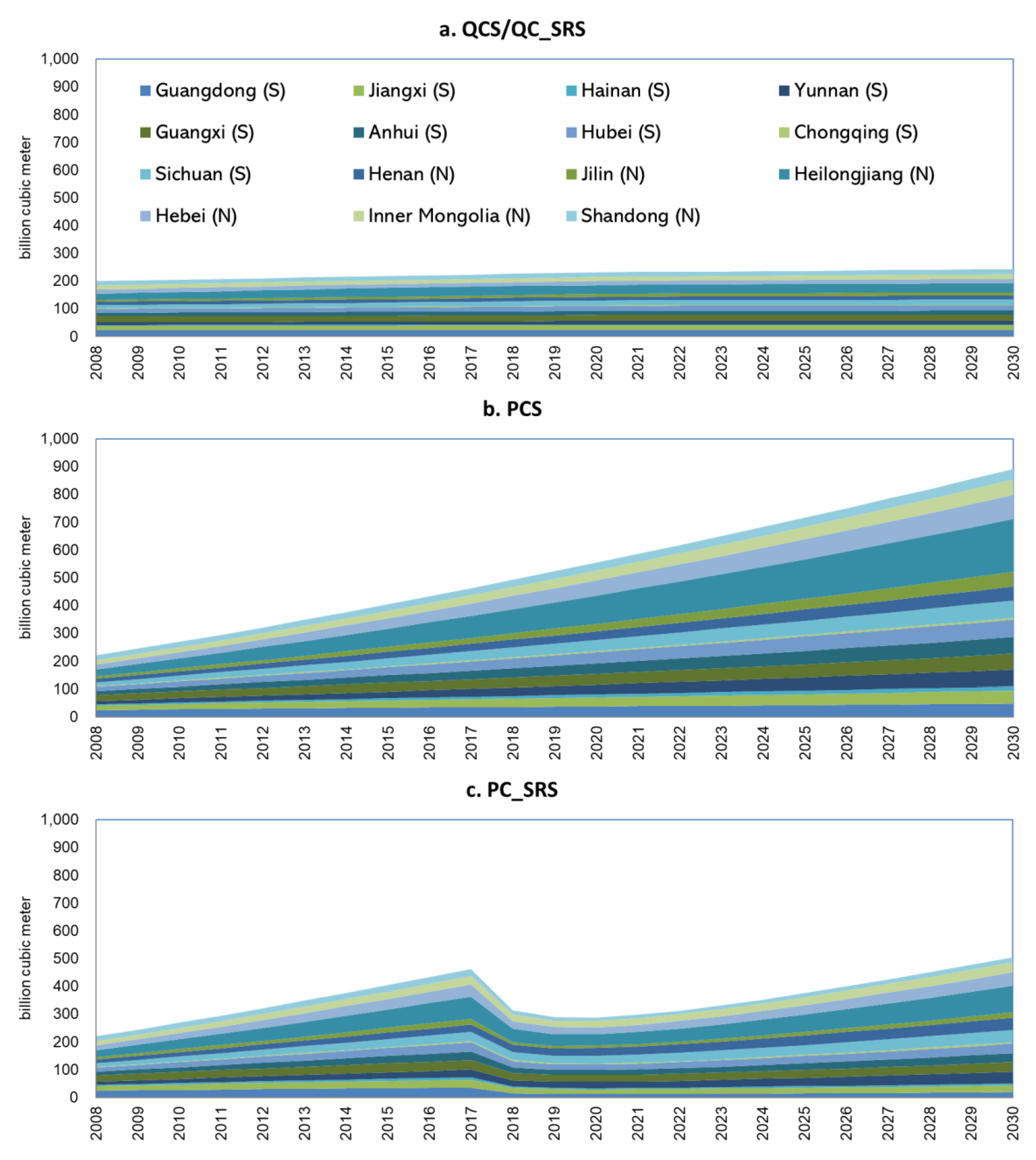
Figure 7 shows that provincial agricultural water deficits, based on the four scenarios, are significant and will differ across provinces between 2020 and 2030. For all 15 selected provinces, agricultural water deficits will increase, especially in Heilongjiang, Hebe, and Inner Mongolia. Moreover, with PC-SRS, agricultural water use in all 15 selected provinces will be significantly reduced in 2018 and 2019, and will then experience a lower growth rate from 2018 to 2030.

4.2. Effects on Farming Production

Table 3. Effects on grain outputs.

Unit: Million Ton	2007 1	2017	2020	2025	2030	Total Growth Rate by 2030, Base Year = 2007)	Annual Growth Rate by 2030 (2007–2030)
Actual data 1	504.14	661.61	---	---	---	---	2.76% 2
QCS	504.14	628.50	675.01	771.03	897.84	78.09%	2.54%
QC-SRS	504.14	628.50	674.81	770.77	897.53	78.03%	2.54%
PCS	504.14	637.18	684.91	783.04	911.87	80.88%	2.61%
PC-SRS	504.14	637.18	678.87	778.80	909.57	80.42%	2.60%

¹ Actual value, data source: National Dataset, available at http://data.stats.gov.cn. ² Actual growth rate between 2007 and 2017 as a reference.

shows effects on different crop outputs according to all policy scenarios, where paddy, wheat, corn, potato, and sorghum are grouped together as a grain. With QCS and PCS, grain outputs increase by 78.09% and 80.88%, respectively, based on the 2015 level. With QCS and QC-SRS, grain output will be 897.84 million tons in 2030, with an annual growth rate of 2.54%. Compared to PCS, PC-SRS limits grain output growth until 2030, but, with an annual growth rate, it was reduced by only 0.01%. Reducing the subsidy creates an insignificant negative effect on grain output. Therefore, the water-saving policy of subsidy reduction does not create a more serious food security problem under conditions of significant reduction in agricultural water use.

As shown in

Table 4. Table effects on different crop outputs.

Unit: Million Ton	2020				2030
	QCS	QC-SRS	PCS	PC-SRS	QCS	QC-SRS	PCS	PC-SRS
Paddy	230.52	231.10	237.59	233.01	276.17	276.94	286.28	284.34
Wheat	146.46	145.65	147.96	147.32	188.50	187.36	190.57	190.50
Corn	251.54	251.56	251.76	251.64	392.76	392.79	393.05	393.01
Potato	20.34	20.35	20.28	20.31	18.62	18.63	18.52	18.55
Sorghum	1.42	1.42	1.43	1.42	1.61	1.62	1.63	1.63
Vegetables	613.74	613.64	620.80	615.67	860.04	859.86	871.26	867.87
Fruits	308.06	308.55	308.60	308.52	492.55	493.51	493.38	493.63
Oil Seeds	4.88	4.88	4.83	4.86	2.31	2.32	2.28	2.29
Sugarcane	152.42	152.61	152.62	152.54	157.54	157.88	157.71	157.71

, only two crops known as wheat and vegetables suffer small output losses when the irrigation subsidy is reduced in QCS, compared with QC-SRS. However, all crops, with the exception of potato and oil seed, suffer output losses in PCS in 2020, and with the exception of potato, sorghum, fruits, oil seeds, and sugarcane suffer losses in 2030. Consequently, higher water prices do not contribute significant pressure to the production of most crops, and even improve production of some crops, especially under QCS conditions.

4.3. Effects on Multi-Provincial Rural Households

At the macro level, results show no significant differences in the impact on rural households or incomes, with regard to either total consumption or welfare (

Table 5. Macro level effects to rural households.

Unit: Annual Growth Rate (%, 2017–2030, Base Year = 2017)	QCS	QC-SRS	PCS	PC-SRS
Income	18.25	18.25	18.28	18.26
Total consumption	10.06	10.06	10.06	10.06
Grain consumption	2.13	2.13	2.19	2.15
Welfare	12.43	12.43	12.43	12.43

). In 2030, PCS will support those rural households with the highest level of grain consumption, but there will be no changes to rural household welfare.

In all scenarios for 2030, the impact on the welfare of rural households differs according to the province. In QCS, the three provinces with the greatest rural household improvements are Guangdong (with an annual growth rate of 12.80%), Henan (12.52%), and Shandong (0.52%). Reducing the subsidy does not create any welfare losses, even though some provinces will see a reduction in grain consumption, as shown in QC-SRS. However, relative to the impact of PCS, under conditions of PC-SRS, there will be a negative but not significant impact on the welfare of rural households. One reason for this is the more than 3% loss in annual grain consumption growth rates (see

Table 6. Effects on rural household welfare and grain consumption.

Unit: Annual Growth Rate (%, 2017–2030, Base Year = 2017)	Changes in Provincial Rural Household Welfare				Changes in Provincial Rural Household Grain Consumption
	QCS	QC-SRS	PCS	PC-SRS	QCS	QC-SRS	PCS	PC-SRS
Guangdong (S)	12.80	12.80	12.80	12.78	2.08	2.07	2.13	2.09
Jiangxi (S)	12.13	12.13	12.12	12.10	1.66	1.65	1.72	1.67
Hainan (S)	12.38	12.38	12.38	12.35	1.94	1.93	2.01	1.95
Yunnan (S)	12.35	12.34	12.36	12.34	2.57	2.56	2.62	2.59
Guangxi (S)	12.01	12.01	12.01	11.99	1.79	1.78	1.85	1.81
Anhui (S)	12.25	12.25	12.26	12.25	1.96	1.95	2.02	1.98
Hubei (S)	12.32	12.32	12.33	12.31	2.03	2.02	2.09	2.05
Chongqing (S)	12.24	12.24	12.24	12.23	2.33	2.32	2.38	2.35
Sichuan (S)	12.11	12.11	12.11	12.10	1.82	1.81	1.88	1.84
Henan (N)	12.52	12.53	12.55	12.54	1.94	1.94	2.02	1.98
Jilin (N)	12.06	12.06	12.09	12.05	2.40	2.40	2.45	2.41
Heilongjiang (N)	12.17	12.17	12.20	12.17	2.59	2.59	2.66	2.61
Hebei (N)	12.49	12.49	12.51	12.49	3.02	3.02	3.05	3.02
Inner Mongolia (N)	12.30	12.30	12.31	12.29	2.85	2.84	2.88	2.85
Shandong (N)	12.52	12.52	12.53	12.51	4.05	4.06	4.05	4.04

).

5. Discussion

Other research in this field supports quantity control over price control as the most effective way to reach 2030 water planning targets. Shi et al. [11], for example, argue that quantity control is a more suitable choice in the Chinese context, while Aarnoudse et al. [43] have found the water quota more effective for groundwater conservation in research conducted in two Chinese counties. There are reasons why these findings may differ from the findings of this research: 1) long-term effects were evaluated to reveal the advantage of quantity control as a water-saving policy and 2) an assumption of general equilibrium was made, where the entire economic system, including both supply and demand, was considered in the model. Overall, the long-term setting and general equilibrium assumption led to different conclusions. On the one hand, an irrigation water price that includes a heavy subsidy will eventually place constraints on increasing the price of agricultural products, which results in farmers reducing grain output. On the other hand, reducing the subsidy is dependent on the precondition that food consumption no longer plays an important role in total consumption, which means that food consumers, including food manufacturers and households, benefitting from long-term economic growth, can afford an increase in food prices resulting from higher water prices. Overall, it is expected that an efficient water pricing mechanism will distribute agricultural water in the long-term. Therefore, this reconciles the growth of grain output with the welfare of rural households. This situation already exists in urban areas and could possibly extend to rural areas to realize the Chinese goal of both urban and rural affluence.

This research has a number of limitations, which should be addressed. Additional data, more field surveys, and more interviews with farmers and water policy makers are required. First, farming sectors should be subdivided at the provincial level to reflect local grain production capacity. Second, provincial water-saving policies should take into consideration the local geography and climate, as well as local labor, water, and technological characteristics. Third, this research has not paid attention to non-agricultural water planning, which has been exerting increasing pressure since the 1980s, due to the increasing water demands of rapid urbanization and industrialization. Despite these limitations, this research offers the potential to improve analysis, and, thus, further develop the model in order to achieve water conservation while improving the welfare of rural households.

6. Conclusions

Relying on a dynamic CGE model, this study sought to investigate how agricultural water conservation, grain production, and the welfare of rural households would be affected by a water-saving policy integrated with the ongoing reduction in irrigation subsidies between 2018 and 2030. Specifically, water planning is designed as a long-term quantitative target. According to these results, it can be inferred that 1) a water-saving policy based on reducing the irrigation subsidy would not have significant impacts on agricultural production, rural household welfare and consumption, and 2) price control would lead to a large increase in agricultural water demand, which is far beyond the quantitative planning target set for 2030.

This research contributes to an expanding body of research that reveals the interactive effects on agricultural production, factor input, and changes to rural household consumption and welfare, that are generated in the process of achieving sustainable goals. Differences in the performance of quantitative and price control mechanisms were evaluated to quantitatively understand the impact of the water-saving policy. Reducing the irrigation subsidy is an important means to promote water saving in crop production within the mechanism of price control. This mechanism continues to play a dominant role in some agricultural areas of China, especially in western and northeastern regions. The results of the research can provide guidance for water-deficient regions of China, where the quantitative control mechanism is used to follow long-term water planning to mitigate serious losses in agricultural outputs and reductions in rural household consumption and welfare. The research can also prove useful outside of China, in countries experiencing a similar dilemma of effecting water policy reform that is not detrimental to agricultural development. The policy modeling process presented here, together with the findings of this research, can be used as a reference for future decision-making.

References

- Ganter, C. Water Crises Are a Top Global Risk. World Economic Forum. 2015. Available online: https://www.weforum.org/agenda/2015/01/why-world-water-crises-are-a-top-global-risk/ (accessed on 20 March 2019).
- United Nations (UN). Goal 6: Ensure Access to Water and Sanitation for All. Available online: https://www.un.org/sustainabledevelopment/water-and-sanitation/ (accessed on 18 April 2019).
- United Nations (UN). International Decade for Action on Water for Sustainable Development, 2018–2028. Available online: https://www.un.org/en/events/waterdecade/ (accessed on 18 April 2019).
- FAO. Coping with Water Scarcity: An Action Framework for Agriculture and Food Security. FAO Water Reports. 2008, p. 38. Available online: http://www.fao.org/3/a-i5604.pdf (accessed on 20 March 2019).
- Poff, N.L.R.; Zimmerman, J.K.H. Ecological responses to altered flow regimes: A literature review to inform the science and management of environmental flow. Freshw. Biol. 2010, 55, 195–205. [Google Scholar] [CrossRef]
- FAO. Country Profiles: China. 2017. Available online: http://www.fao.org/countryprofiles/index/en/?iso3=chn (accessed on 10 March 2019).
- Qin, C.B.; Su, Z.A.; Bressers, H.T.; Jia, Y.W.; Wang, H. Assessing the economic impact of North China’s water scarcity mitigation strategy: A multi-region, water-extended computable general equilibrium analysis. Water Int. 2013, 38, 701–723. [Google Scholar] [CrossRef]
- Deng, X.P.; Shan, L.; Zhang, H.; Turner, N.C. Improving agricultural water use efficiency in arid and semi-arid areas of China. Agric. Water Manag. 2006, 80, 23–40. [Google Scholar] [CrossRef]
- Jiang, Y. China’s water scarcity. J. Environ. Manag. 2009, 90, 3185–3196. [Google Scholar] [CrossRef] [PubMed]
- UNCED. The Dublin Statement on Water and Sustainable Development. 1992. Available online: http://www.un-documents.net/h2o-dub.htm (accessed on 20 March 2019).
- Shi, M.J.; Wang, X.J.; Yang, H.; Wang, T. Pricing or quota? A solution to water scarcity in oasis regions in China: A case study in the Heihe River Basin. Sustainability 2014, 6, 7601–7620. [Google Scholar] [CrossRef]
- Wang, G.; Liu, C.; Wang, J. Situation confronted by reform of agricultural water pricing system and lessons learned home and abroad. China Water Resour. 2015, 18, 14–17. (In Chinese) [Google Scholar]
- Li, C.Y.; Wang, H.M.; Tong, J.P.; Liu, S. Water Resource Policy Simulation and Analysis in Jiangxi Province Based on CGE Model. Resour. Sci. 2014, 36, 84–93. (In Chinese) [Google Scholar]
- Zhong, S.; Sha, J.H.; Shen, L.; Okiyama, M.; Tokunaga, S.; Yan, J.J.; Liu, L.T. Measuring drought based on a CGE Model with multi-regional irrigation water. Water Policy 2016, 18, 877–891. [Google Scholar] [CrossRef]
- Shen, M.; Zhong, S.; Shen, L.; Liu, L.T.; Zhang, C. Comparative Evaluation between Water Parallel Pricing System and Water Pricing System in China: A Simulation of Eliminating Irrigation Subsidy. J. Resour. Ecol. 2016, 7, 237–246. [Google Scholar] [CrossRef]
- Ge, J.P.; Lei, Y.L.; Tokunaga, S. Non-grain fuel ethanol expansion and its effects on food security: A computable general equilibrium analysis for China. Energy 2014, 65, 346–356. [Google Scholar] [CrossRef]
- Okiyama, M.; Tokunaga, S. Impact of expanding bio-Fuel consumption on household income of farmers in Thailand: Utilizing the computable general equilibrium model. Rev. Urban Reg. Dev. Stud. 2010, 22, 109–142. [Google Scholar] [CrossRef]
- Tokunaga, S.; Resosudarmo, B.P.; Wuryanto, L.E.; Dung, N.T. An inter-regional CGE Model to assess the impacts of tariff reduction and fiscal decentralization on regional economy: The case of Indonesia. Stud. Reg. Sci. 2003, 33, 1–25. [Google Scholar] [CrossRef]
- The State Council. National Agricultural Water-Savings Program 2012–2020. 2011. Available online: http://www.gov.cn/zwgk/2012-12/15/content_2291002.htm (accessed on 10 November 2018).
- The State Council. Direction to Implementing the Most Stringent Water Management System. 2012. Available online: http://www.mwr.gov.cn/ztpd/2012ztbd/szyzt/ (accessed on 10 November 2018).
- Huang, Q.; Wang, J.; Easter, K.W.; Rozelle, S. Empirical assessment of water management institutions in northern China. Agric. Water Manag. 2010, 98, 361–369. [Google Scholar] [CrossRef] [Green Version]
- Huang, Q.Q.; Rozelle, S.; Howitt, R.; Wang, J.X.; Huang, J.K. Irrigation water demand and implications for water pricing policy in rural China. Environ. Dev. Econ. 2010, 15, 293–319. [Google Scholar] [CrossRef]
- Han, H.Y.; Zhao, L.G. The Impact of Water Pricing Policy on Local Environment—An Analysis of Three Irrigation Districts in China. Agric. Sci. China 2007, 6, 1472–1478. [Google Scholar] [CrossRef]
- Yang, H.; Zhang, X.; Zehnder, A.J.B. Water scarcity, pricing mechanism and institutional reform in northern China irrigated agriculture. Agric. Water Manag. 2003, 61, 143–161. [Google Scholar] [CrossRef]
- Tsur, Y.; Roe, T.; Doukkali, R.; Dinar, A. Pricing Irrigation Water: Principles and Cases from Developing Countries; Resources for the Future: Washington, DC, USA, 2004. [Google Scholar]
- Zhong, S.; Shen, L.; Sha, J.H.; Okiyama, M.; Tokunaga, S.; Liu, L.T.; Yan, J.J. Assessing the Water Parallel Pricing System against Drought in China: A Study Based on a CGE Model with Multi-Provincial Irrigation Water. Water 2015, 7, 3431–3465. [Google Scholar] [CrossRef]
- Qu, F.; Kuyvenhoven, A.; Shi, X.; Heerink, N. Sustainable natural resource use in rural China: Recent trends and policies. China Economic Review. 2011, 22, 444–460. [Google Scholar] [CrossRef]
- Cremades, R.; Wang, J.; Morris, J. Economic incentives and the adoption of modern irrigation technology in China. Earth Syst. Dyn. 2015, 6, 399–410. [Google Scholar] [CrossRef]
- Wang, J.X.; Huang, J.K.; Rozelle, S.; Huang, Q.Q.; Zhang, L.J. Understanding the water crisis in Northern China: What the government and farmers are doing. Int. J. Water Resour. Dev. 2009, 25, 141–158. [Google Scholar] [CrossRef]
- Mamitimin, Y.; Feike, T.; Seifert, I.; Doluschitz, R. Irrigation in the Tarim Basin, China: Farmers’ response to changes in water pricing practices. Environ. Earth Sci. 2015, 73, 559–569. [Google Scholar] [CrossRef]
- Zhong, L.; Mol, A.P.J. Water Price Reforms in China: Policy-Making and Implementation. Water Resour. Manag. 2009, 24, 377–396. [Google Scholar] [CrossRef] [Green Version]
- Liao, Y.S.; Gao, Z.Y.; Bao, Z.Y.; Huang, Q.W.; Feng, G.Z.; Xu, D.; Cai, J.B.; Han, H.J.; Wu, W.F. China’s Water Pricing Reforms for Irrigation: Effectiveness and Impact; International Water Management Institute: Colombo, Sri Lanka, 2008. [Google Scholar]
- Cai, X. Water stress, water transfer and social equity in Northern China—Implications for policy reforms. J. Environ. Manag. 2008, 87, 14–25. [Google Scholar] [CrossRef]
- Latinopoulos, D. Estimating the Potential Impacts of Irrigation Water Pricing Using Multicriteria Decision Making Modelling. An Application to Northern Greece. Water Resour. Manag. 2008, 22, 1761–1782. [Google Scholar] [CrossRef]
- Aregay, F.A.; Zhao, M.J.; Bhutta, Z.M. Irrigation water pricing policy for water demand and environmental management: A case study in the Weihe River basin. Water Policy 2013, 15, 816–829. [Google Scholar] [CrossRef]
- Wang, X.Y. Irrigation Water Use Efficiency of Farmers and Its Determinants: Evidence from a Survey in Northwestern China. Agric. Sci. China 2010, 9, 1326–1337. [Google Scholar] [CrossRef]
- Liu, J.G.; Zang, C.F.; Tian, S.Y.; Liu, J.G.; Yang, H.; Jia, S.F.; You, L.Z.; Liu, B.; Zhang, M. Water conservancy projects in China: Achievements, challenges and way forward. Glob. Environ. Chang. 2013, 23, 633–643. [Google Scholar] [CrossRef] [Green Version]
- Xiong, W.; Conway, D.; Lin, E.; Xu, Y.L.; Ju, H.; Jiang, J.H.; Holman, I.; Li, Y. Future cereal production in China: The interaction of climate change, water availability and socio-economic scenarios. Glob. Environ. Chang. 2009, 19, 34–44. [Google Scholar] [CrossRef]
- Lohmar, B.; Wang, J.; Rozelle, S.; Huang, J.; Dawe, D. China’s Agricultural Water Policy Reforms: Increasing Investment, Resolving Conflicts, and Revising Incentives; Agriculture Information Bulletin No. 782; Economic Research Service, US Department of Agriculture: Washington, DC, USA, 2003.
- Zhong, S.; Shen, L.; Liu, L.; Zhang, C.; Shen, M. Impact analysis of reducing multi-provincial irrigation subsidies in China: A policy simulation based on a CGE model. Water Policy 2017, 19, 216–232. [Google Scholar] [CrossRef]
- Berrittella, M.; Rehdanz, K.; Richard, S.J.T. The Economic Impact of the South-North Water Transfer Project in China: A Computable General Equilibrium Analysis. FEEM Working Paper 154. 2006. Available online: http://www.fnu.zmaw.de/fileadmin/fnu-files/publication/working-papers/cgewaterchinawp.pdf (accessed on 1 November 2016).
- Qin, C.; Bressers, H.T.; Su, Z.B.; Jia, Y.; Wang, H. Assessing economic impacts of China’s water pollution mitigation measures through a dynamic computable general equilibrium analysis. Environ. Res. Lett. 2011, 6, 044026. [Google Scholar] [CrossRef] [Green Version]
- Aarnoudse, E.; Qu, W.; Bluemling, B.; Herzfeld, T. Groundwater quota versus tiered groundwater pricing two cases of groundwater management in north-west China. Int. J. Water Resour. Dev. 2017, 33, 917–934. [Google Scholar] [CrossRef]
Figure 1.
Location of the selected 15 provinces in China.
Figure 2.
Flow chart of agricultural water policy simulation according to the dynamic CGE model.
Figure 3.
Historical changes in outputs and planting areas of China’s nine primary crops. Data source: National Dataset, available at http://data.stats.gov.cn.
Figure 4.
Historical changes in agricultural water use and crop planting areas in the 15 provinces. Data source: National Dataset, available at http://data.stats.gov.cn.
Figure 5.
Historical changes in rural labor migration in the 15 provinces. Data source: National Dataset, available at http://data.stats.gov.cn.
Figure 6.
Total agricultural water use, according to all scenarios.
Figure 7.
Changes in provincial irrigation water use, according to all scenarios.