Optimization and Application of Integrated Land Use and Transportation Model in Small- and Medium-Sized Cities in China

1
School of Highway, Chang’an University, Xi’an 710000, China
2
Zhejiang Jinquli Natural Gas Company Co., Ltd., Hangzhou 310016, China
*
Author to whom correspondence should be addressed.
Sustainability 2019, 11(9), 2555; https://doi.org/10.3390/su11092555
Submission received: 24 January 2019
/
Revised: 26 April 2019
/
Accepted: 29 April 2019
/
Published: 2 May 2019
(This article belongs to the Special Issue Urban Sprawl and Sustainability)
Abstract
:Integrated land use and transportation models are helpful when policy, planning, or environment impacts are being evaluated, but the strengths and limitations in these models must be optimized. To optimize the ITLUP (Integrated Transportation and Land-Use Planning) model and apply it in small- and medium-sized cities in China, this study considered the constraints of land use intensity and introduced two critical indicators (the maximum number of households and maximum employment) to characterize the land capacity and improve the practicality of the model. Then, Monte Carlo simulation analysis was used to analyze the uncertainty factors using the coefficient of variation (C.V) and standardized regression coefficient (SRC). The results suggest that the maximum future employment and households may exceed the land limit and must be adjusted to a new zone, and the model operation simulation was closer to the actual situation of small- and medium-sized cities. The C.V value of the model output showed the increasing trend of the uncertainty of the model output variable over time, especially affected by DRAM model parameters, traffic demand forecasting model parameters and the peak hourly flow ratio. Such findings are meaningful for policymakers, planners, and others when the ITLUP model is used to anticipate the zonal employment and household allocation and to further explore the interaction between land use and transportation.
1. Introduction
China is now in a rapid development period of motorization and urbanization, and green, smart, safe and sustainable urban development is an inevitable trend. Land is the carrier of all human production and life; its structure, mode and dynamic changes affect the operation of the entire city. Land carrying capacity, land use intensification, and land structure complexity are all issues that need to be considered in city planning around land usage. Transportation is the skeleton of urban operation and also profoundly affects the cities’ sustainable development. The integration of land use and transportation development is the focus of urban planners.
The interaction between land use patterns and travel behaviors has been recognized for decades in the literature [1]. The general relationship between transportation and land-use may be defined in terms of three primary components: economic activity (i.e., employment), demographic activity and transportation facilities [2]. Understanding the interactions and mechanisms is of great significance to build well-organized urban space organizations and alleviate urban transport problems. ITLUMs (Integrated Transport-Land Use Models) enable analysts to anticipate the system response to new policies, preference functions, economic conditions and other scenarios.
Several ITLUMs have been applied to date and are publicly available in practice [3,4,5,6,7,8,9,10,11,12]. Lowry’s Model of Metropolis is the first attempt to implement an urban land use traffic feedback cycle in the operating model, which is the basis for most subsequent research and has stimulated many increasingly complex modeling methods [3]. Putman found that nonlinear mathematical programming formulations of a combined model of the location, trip-making, and trip assignment can effectively avoid model convergence problem [13,14]. The MEPLAN framework was most applicable in situations where consistent land use and transport predictions and evaluations are required due to its various strengths, especially where there are relatively few observed data points [15]. Kockelman et al. explored a random-utility-based multiregional IO (RUBMRIO) model based on spatial IO theories and applied it in Texas, which provides a valuable set of relationships and can be used to predict the trade flows, location choices/production levels, and relative market prices [16]. SLEUTH (Slope, Land Use, Excluded, Urban, Transportation and Hillshade model) is a computational simulation model that uses adaptive cellular automata to simulate the way cities grow and change their surrounding land uses, while the analysis process usually lack combination with the local city development characteristics [10,17,18]. However, based on the demographic, policy, economic and market changes, the strengths and limitations of these models are present in the context of data requirements, model calibration, result presentation, etc. [19,20,21,22,23]. In addition, the spatial resolution of present models is still too coarse to model neighborhood scale policies and effects [24].
ITLUP (Integrated Transportation and Land-Use Planning) and UrbanSIM (Urban Simulation Model) are two typical procedures to explore the relationship between transportation and land use [25,26] and have been widely used in practice [27]. These two land use models were compared based on data requirements, calibration, and result presentation [1]. The results show that the highly aggregate data required for ITLUP (which seeks to simulate the development of individual parcels and the decisions of individual households and firms [9]) are relatively easy to gather, whereas the disaggregate data required for UrbanSim may take months or even a few years to refine to an acceptable level of reliability [1,24] and are more extensive [28]. The Bayesian Melding calibration method under development by the UrbanSim team provides great convenience to users, who otherwise must rely on statistical software and have expert knowledge of the estimation process. However, it requires two or more years of data, which implies that full calibration may not be possible. The data required for the ITLUP model calibration are more readily available. There are numerous options to present the results for UrbanSim, whereas the ITLUP model is very limited in its presentation capabilities. In general, ITLUP is a simple model with less flexibility, and UrbanSim is a complex model with more flexibility. The data required for ITLUP are easier and less expensive to gather than that for UrbanSim.
There are great differences in the status quo of land use and transportation development in China’s big as well as small- and medium-sized cities. At the same time, there are many restrictions on the development of small- and medium-sized cities (here, this usually refers to counties, which are the third part of the administrative division of China; there are 2876 counties in China in 2018) in China. In view of the limitations (fewer available statistical data) of small- and medium-sized cities in China that may exist in the rapid urbanization process and Duthie’s comparison results of ITLUP and UrbanSim in data requirements and model calibration, this study selected the ITLUP model to analyze the relationship between land use and transportation systems. Moreover, from the perspective of functional positioning and sustainable development of small- and medium-sized cities in China, it is not necessary to carry out high-intensity urban land development. Therefore, this study regarded environmental capacity as an important factor in the planning of land use in small- and medium-sized cities and introduced two indicators (maximum number of households and maximum employment) to improve the practicality. In addition, considering the dynamics and complexity of urban planning and traffic planning, policy may have changes over time, which in turn affects the input variables and has an uncertain effect on the output of the model. Thus, this study explored the uncertainty of input variables and parameters. The above forms the main component of Section 2, which is followed by a description of the results, a discussion, and the conclusion.
2. Methods and Data
Compared with big cities, the level of land intensification in small- and medium-sized cities in China is generally low. Furthermore, the transportation system in small- and medium-sized cities in China has several main characteristics: usually lower per capita road area (not always); insufficient public transportation system in route scale, density and operating kilometers; lack of consistency between urban land use and transportation systems; and disjointed or semi-detached land use planning and traffic planning [27].
Considering the traffic development situation and the difficulty in obtaining enough data in small- and medium-sized cities in China, and comprehensive consideration of model data, calibration methods and prediction results, we chose the ITLUP model for research. The ITLUP model mainly includes a land use model and a traffic demand forecast model. The land use model consists of EMPAL (Employment Allocation Model) and DRAM (Disaggregate Residential Allocation Model) [29]. The ITLUP model provides an interactive feedback mechanism for EMPAL, DRAM and traffic demand forecast model.
2.1. Components of the ITLUP Model
2.1.1. Land Use Model and Its Application
(1) EMPAL
EMPAL (Employment Allocation Model) is applied to predict the future zonal distribution of employment. Its formulation includes two parts: the zonal employment growth of a specific zone and the employment attracted from other zones. The formulation is shown in Equation (1):
where the term on the left side of the plus sign denotes the employment attracted to zone j in time period t; the term on the right side of the plus sign refers to the employment growth of zone j in time period t; is the future distribution of employment in zone j in time period t; is the zonal households of all types in zone i in the previous time period t − 1; is the zonal employment attraction function in the previous time period t − 1; is the peak travel time from zone j to zone i in time period t; is the off-peak travel time from zone j to zone i in time period t − 1; is the ratio of total employment in time period t to total number of households in previous time period t − 1 of the entire area; is the ratio of total employment in time period t to total employment in previous time period t − 1 of the entire area; and , , and are empirical parameters.
The zonal employment attraction function is expressed as Equation (2):
where is area of zone ; and and are empirical parameters.
Due to the characteristics (e.g., mainly labor-intensive urban industry and relatively low proportion of the service industry and its land use) of the small- and medium-sized cities in China, this study divided jobs into three types: basic, commercial and service employment.
(2) DRAM
DRAM (Disaggregate Residential Allocation Model) is applied to predict the future zonal distribution of households and formulated as shown in Equation (3):
where the part in the bracket denotes the zonal household attraction; is the household forecast of zone i in time period t; is the zonal household attraction function in time period t; and is the ratio of total household to total employment in time period t of the entire area.
The zonal household attraction function is expressed in Equation (4):
where is the area of zone i in time period t; and and are empirical parameters.
This study divided the households into three types according to their annual income: low, medium and high income.
2.1.2. Travel Demand Model and Its Application
Travel demand forecasting in the ITLUP model is based on the traditional four-step model:
- (1)
- Trip generation analysis: Estimate the number of trips that a person or vehicle makes in a particular location (usually a zone). It is assumed that the trip production is a linear function of the number of households, and the trip attraction is linear with employments.
- (2)
- Double-constraint gravity model: Predict trip distribution [29].
- (3)
- Multinomial Logit Model: Predict the sharing rate of different traffic modes. Then, the trip distribution is multiplied with the sharing rate to obtain the trip distribution of different traffic modes. The distribution of peak/off-peak travel hours is calculated according to the trip distribution rates of peak/off-peak travel hours.
- (4)
- SUE (Stochastic User-Optimized Equilibrium) in TransCAD: Assign the trips of peak travel hours and off-peak hours in the road network [29]. The travel time estimation is based on the BPR function, and the road network is mainly divided into three types.
2.2. Optimization Method of the ITLUP Model
Through careful analysis and research on the ITLUP model, it can be found that the model has certain limitations: (1) the model does not consider land use intensity constraints, it allocates employment and families to the area even if they do not have enough capacity; (2) the EMPAL and DRAM models are applied sequentially, ignoring the interaction between employment and household; and (3) the ITLUP model does not consider the impact of land prices and commodity trade on employment and household distribution. This limitation will have a greater impact on the application of the model in large cities, while the impact is small in small- and medium-sized cities in China [22]. Therefore, for small- and medium-sized cities, the limitations are mainly reflected in the lack of consideration of urban land capacity. Thus, this study introduced two indicators to illustrate the environmental capacity: maximum number of households and maximum employment.
(1) Maximum number of households
The maximum number of households is the number of households (assume average three persons per household) in a residential area when the residential land per capita reaches the minimum acceptable range. It is formulated as Equation (5):
where is the maximum number of households that zone i can accommodate; is the total area of zonal residential land; and is the minimum acceptable residential land per capita.
(2) Maximum employment
Employment can be divided into basic, commercial and service employment. We analyzed the maximum employment quantity.
The zonal maximum employment on industrial land is the number of employees when the per capita land area reaches the minimum value. It is expressed as Equation (6):
where is the zonal maximum basic employment; is the total industrial land area in zone ; and is the minimum industrial land per capita.
The population of different public facilities consists of two parts: employment and customers. Thus, the zonal maximum employment is equal to the population (when the per capita land area is minimal) multiplied by the ratio of employment to trip attraction. The maximum commercial and service employment are expressed as Equations (7) and (8), respectively:
where is the zonal maximum commercial employment; is the total commercial land area in zone i; is the minimum commercial land per capita (it can be defined by Urban public facilities planning norms GB50442-2008); and is the ratio of the commercial employment to trip attraction of each zone.
where is the zonal maximum of other service employment; is the total land area of type z in zone i (z = 1, 2, 3, where 1 indicates administrative land, 2 indicates medical land, and 3 indicates education land); is the minimum land area per capita of type z; and is the ratio of type-z employment to trip attraction in zone i.
By studying the application and optimization methods of the ITLUP model, the basic frame of the improved ITLUP model is shown in Figure 1.
2.3. Uncertainty Analysis of the ITLUP Model
2.3.1. Quantitative Method of Uncertainty Factors of the ITLUP Model
(1) Determining the probability distribution of the input variables and parameters
According to the empirical and historical data and considering the input variables and parameter characteristics of the ITLUP model, we selected the suitable probability distribution for the input variables and parameters. In each part of the prediction model, many variables can only change in the nonnegative range. To avoid the negative number in the process of generating random numbers, we used the lognormal distributions to represent the input variables and parameters [30]. We chose the multivariate log-normal distribution to represent the probability distribution of the input variables and parameters of the ITLUP model.
The log-normal distribution probability density function is shown with location parameter and shape parameter as follows:
where is the mean value of the location parameter after the logarithm, which is called the logarithmic mean; and is the shape after the logarithm of the probability density curve, which is called the logarithmic standard deviation.
The coefficient of variation (C.V) is formulated as Equation (10):
(2) Determining the C.V of the input variables and parameters
The C.V was chosen as the expression variable for the uncertainty of the input variables and parameters. In general, the C.V of some input variables cannot be directly determined. According to the study of Kockelman and related scholars [31], the C.V of an input value is assumed to be 0.3. Thus, we could calculate their standard deviation by multiplying the mean model inputs by the coefficient of variation.
(3) Simulation analysis
The simulation analysis was conducted by @Risk (Monte Carlo simulation software). Monte Carlo simulation software can directly generate random samples according to the probability distribution of input variables and the parameters. It can also calculate the output value and distribution of the model in the random samples.
2.3.2. Uncertainty Analysis Method of the ITLUP Model
The multivariate sensitivity analysis method was used to analyze the uncertainty of the ITLUP model. Based on the linear regression of the input and output, the effect of the model input variables and parameters on the uncertainty of the output variables was analyzed.
(1) Multiple linear regression analysis
Multiple linear regression analysis is a statistical analysis that studies the interrelationship between a dependent variable and multiple independent variables. It assumes that there are P independent variables (X1, X2, …, XP,) and one dependent variable Y. The linear regression function of these variables is shown as Equation (11):
where , , …, are regression coefficients; and is the error term of the mormal distribution N (0, ).
In the uncertainty analysis of the model, a specific output variable can be set as a dependent variable, and the input variables and parameters can be set as independent variables. Then, it combines with Monte Carlo method to calculate the distribution results. The estimated value of the regression coefficients (, , …, ) can be obtained using the SPSS software.
(2) Regression coefficient significance test
Using the SPSS software to test the significance of the regression coefficient, the T value and corresponding P value of can be obtained. If P is less than the significant level (generally 0.05), it implies that is not equal to zero. In other words, the corresponding variable significantly affects the model output variables. If P is greater than 0.05, the corresponding variable will not affect the model output.
(3) Sensitivity analysis
After performing the linear regression analysis and significance test on the input variables for the output variables, we calculated the standardized regression coefficients () using Equation (12):
where is the standardized regression coefficient; is a regression coefficient; is the standard deviation of the independent variable; and is the standard deviation of the dependent variable.
2.4. Data Acquisition
This study considered the main urban area of Huangling County (in Shaanxi province, China) as an example to run the whole optimization method. Referring to the document of “Huangling County Urban Comprehensive Traffic Planning 2014–2030”, the main urban area was divided into nine traffic zones, where Zones 1–7 are the inner zones, and Zones 8 and 9 are the external zones. The population of the main urban area is 35,892. Current zonal land use data, zonal number of household and employment, households type due to household income, employment type, peak and off-peak travel time between zones, travel time and travel expenses of various modes of transportation, annual average growth rate of employment and population were needed to operate this model.
3. Results and Discussion
3.1. Prediction Results of the Model
Based on the survey data and Equations (5)–(8), the maximum allowable number of households and employment in each zone were calculated, and the results are shown in Table A1 and Table A2 (see Appendix A).
The model parameters were calibrated by the data from 2012 and 2014. Assuming that the input C.V was 0.3, the predicted results of all types of employment were obtained. The results are shown in Appendix A.
The prediction results show that, under the effect of the model input and parameter uncertainty, the maximum employment and households in the main urban areas of Huangling County will exceed the land capacity limit index by 2030. The main results are as follows: (1) The whole maximum employment of the largest commercial employment and other services in the main urban areas exceed the land bearing limit (17,980 = 9026 + 8954), which is expected to reach 2967 (1489 + 1478).; (2) The maximum employment of other services exceeds the land bearing limit (8954), which is expected to reach 1478 (see Table A1 in Appendix A). (3) The maximum number of households exceeds the land limit (9782), which is expected to reach 1873 (see Table A2 in Appendix A). (4) The C.V value of the commercial and other service employment (excluding the other service employment in Zone 6) and the number of households in each zone increase compared with the input coefficient variation coefficient (0.3). Therefore, according to the established optimization model, Huangling County must build a new Zone 10 to satisfy the demand growth of the city in terms of population and employment.
As shown in Table A3 in Appendix A, the maximum traffic volume on all roads during peak hours reaches 90% of capacity. In addition, the V/C ratio during peak travel time is 0.9–1.0. Thus, the LOS of the road is E, indicating that the traffic flow is in an unstable state and will result in significant time delays. Therefore, in the follow-up urban planning work, a series of adjustments to the urban space layout and road traffic conditions is necessary. For instance, from the perspective of green transportation and sustainable development, planners can consider optimizing land use mix, urban residential space design, and traffic structure to improve accessibility and reduce carbon emissions.
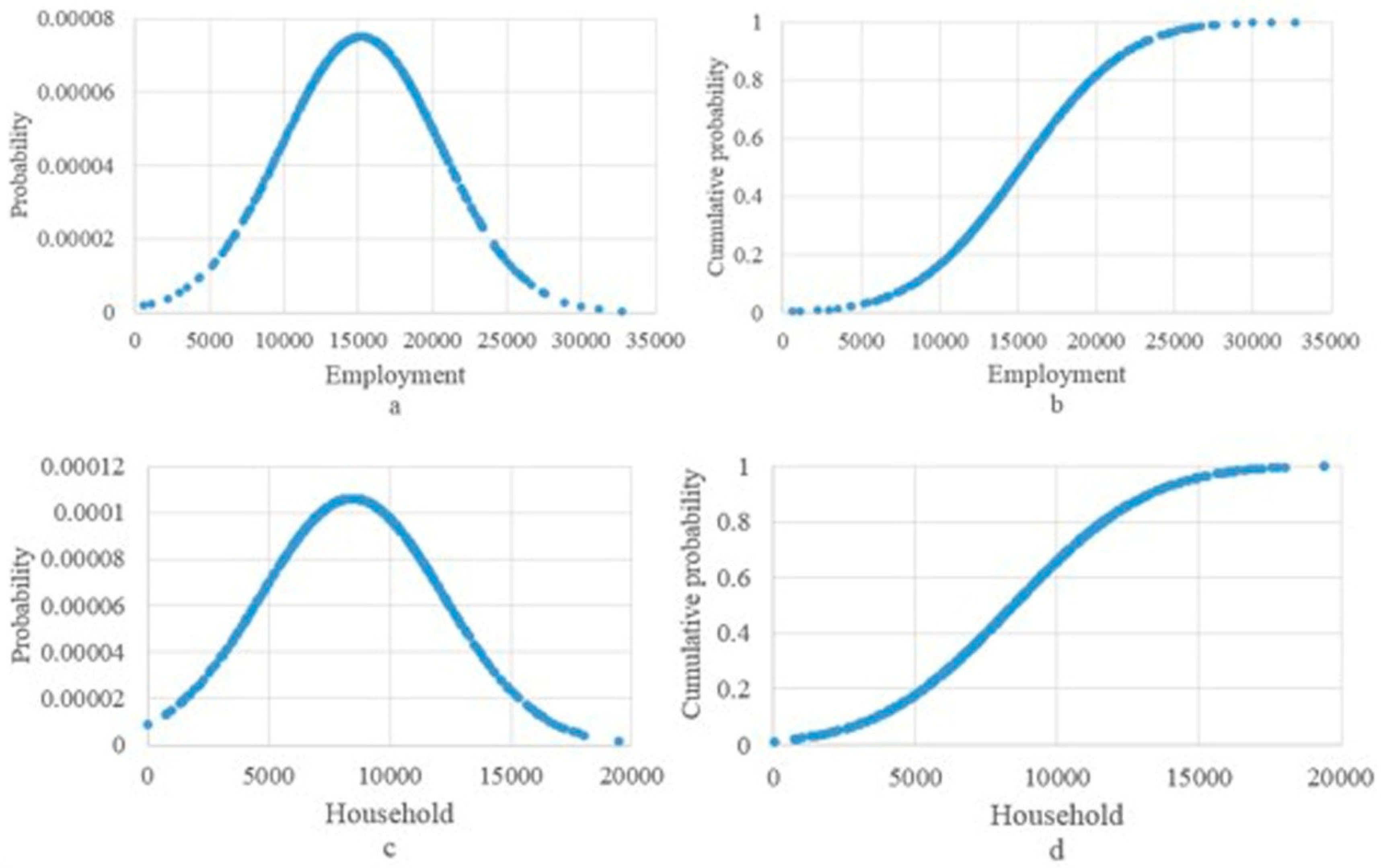
3.2. Prediction Results of Uncertainty Analysis
The multivariate sensitivity analysis was used to analyze the effect of the input changes on the uncertainty of the output, and the standardized regression coefficients were calculated. The statistical distribution of the optimized employment and household after Monte Carlo simulation is shown in Figure 2. The results of the sensitivity analysis are shown in Table A4 and Table A5 in Appendix B.
The sensitivity analysis results show three points. (1) The input with a large impact on the uncertainty of urban employment included the DRAM model parameters. The most influential factors were (SRC = 3.112), (SRC = 0.753), and (SRC = 0.387). In other words, when the level of uncertainty in the input parameters of the DRAM model decreased, the level of uncertainty in the forecast of urban employment also decreased. (2) The input with a large impact on the uncertainty of the household volume included the traffic demand forecasting model parameters, where the most influential factors were (SRC = 0.159) and (SRC = 0.191). In other words, when the level of uncertainty in the parameters of the traffic demand forecasting model decreased, the uncertainty of the model prediction of the household volume also decreased. (3) The uncertainty of the peak hour flow of various roads was mainly affected by the peak hourly flow ratio . The SRC (0.211) of arterial road was the largest, which indicated that it greatly affected the uncertainty of the arterial road flow. The off-peak hour flows were mainly affected by (SRC = 0.231/0.221/0.227), and traffic demand parameters (SRC = 0.179/0.172/0.177) and (K = 1/2/3, corresponding SRC1 = 0.199, SRC2 = 0.190, SRC3 = 0.196). In other words, the uncertainty of the predicted value of the peak hourly flow of each type of road decreased with the decrease in uncertainty of the peak hour flow rate. The uncertainty of the forecast of the off-peak hour flow decreased when the uncertainties of the average population growth rate () and traffic demand parameters decreased ( and ).
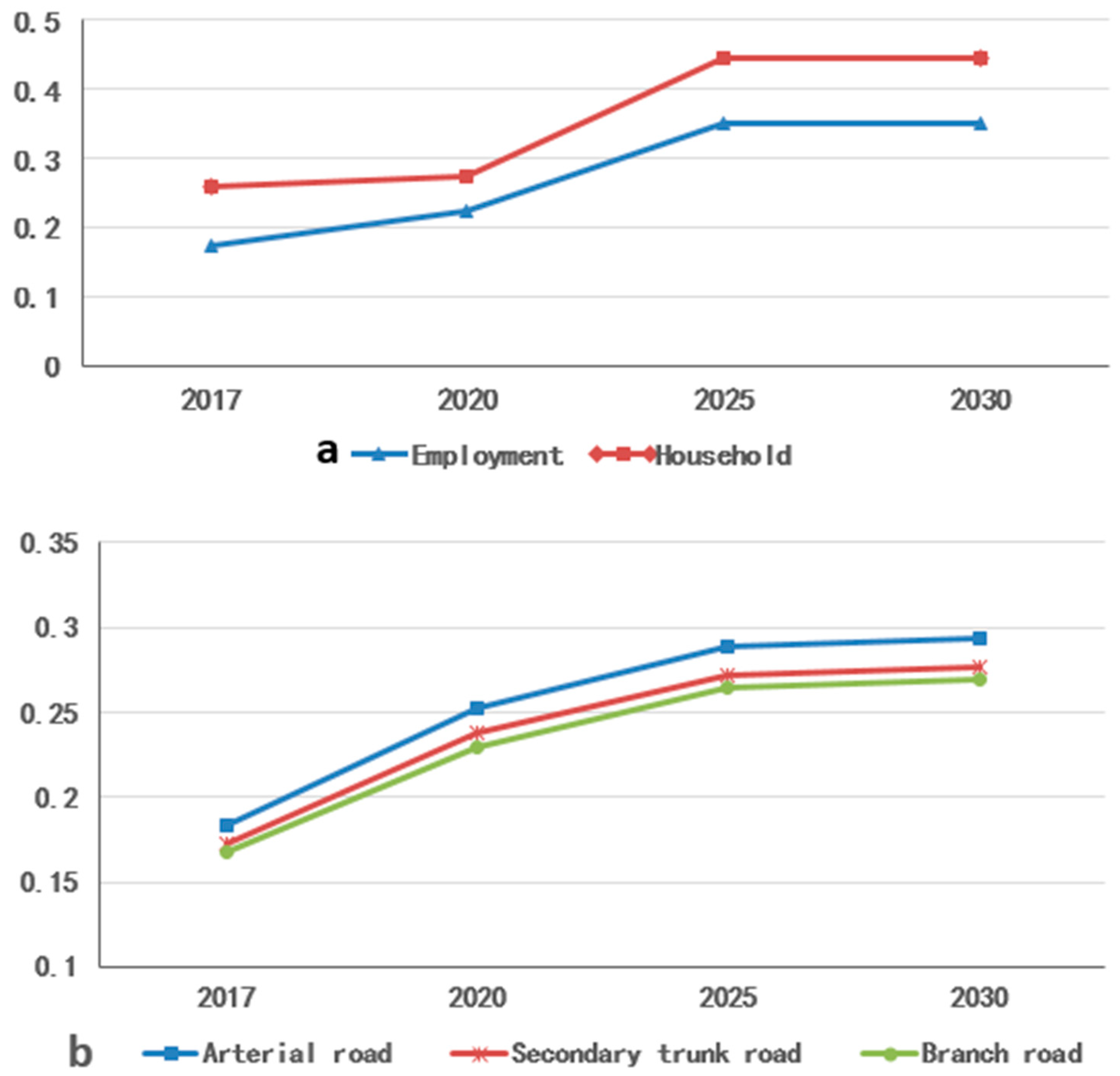
3.3. Analysis of the Uncertainty Propagation Over Time
The C.V of the output was used to study the evolution of the model uncertainty with time. The variation trend of C.V over time is shown in Figure 3.
The C.V of the output variables of the model gradually increased with time. For 2030, the uncertainty levels of employment and households were 35% and 44.5%, respectively. In the future planning process, urban planners should pay more attention to the layout structure of residential areas and pay attention to the flexibility of medium and long-term residential design. The uncertainty levels of the traffic V/C ratios at various road peak times were: arterial road was 29.4%, secondary trunk road was 27.7%, and branch road was 26.9%. Thus, decision makers should pay attention to the balance of different grades of road layout when planning traffic.
4. Conclusions
Based on the characteristics of land use and transportation systems in small- and medium-sized cities, this study selected the ITLUP model as the method and studied its application. By analyzing the limitations of the ITLUP model in application and the development characteristics of small- and medium-sized cities, we introduced two indicators: maximum number of households and maximum employment, to optimize the ITLUP model. Then, by analyzing the sources of uncertainty, the meanings of the model input variables and parameter uncertainties and their effect on the model were expounded. The analysis method of uncertainty of the ITLUP model was established. The effects of the model input variables and parameter changes on the uncertainty of output and evolution of the uncertainty of model predictions over time were studied. The results show that:
- (1)
- Through the introduction of two characteristic indicators, the traditional ITLUP model was optimized for employment and family allocation, and the model operation simulation was closer to the actual situation of small- and medium-sized cities. The prediction results show that the county needs to build a new zone to satisfy the demand growth of the city when zonal land capacity is considered. Thus, it is important to coordinate the relationship between urban development and resource and environment carrying capacity. Planners may analyze the future urban land use development based on the forecast results, and carry out effective resource allocation to provide reference for land structure optimization, green traffic and environmental protection.
- (2)
- The uncertainty of the model output variable gradually increased with time (The C.V value of the model output shows the increasing trend over time). Therefore, when using this model to predict the development of small- and medium-sized cities, it is necessary to ensure the accuracy of these variables, which are DRAM model parameters, traffic demand forecasting model parameters and the peak hourly flow ratio (see Section 3.2). At the same time, the model had great uncertainty for long-term planning, and the prediction for short- and medium-term was more accurate.
The findings of this study emphasize the importance of ITLUMs in the study of integration development of Land use and transportation [12,32,33]. In general, by considering land use restrictions, the introduction of maximum number of households and maximum employment can effectively alleviate the inconsistency between the construction of transportation systems and the pace of urban economic development in the urban development process. Using the optimized model, urban planners can leave a buffer for the short- and medium-term urban construction by measuring the maximum land use restrictions, which can effectively avoid the traffic congestion caused by land tension in future urban developments. This study enriches the practical application in small- and medium-sized cities in China and illustrates the applicability of the ITLUP model, which takes land carrying capacity into account in small- and medium-sized cities. It can also be a reference for future development.
However, the limitations in this study should be recognized. First, the example in the study did not consider the mode of public transportation. The ITLUP model should be applied to the development forecast of other small- and medium-sized cities, and the effect of public transportation development trend and model uncertainty on it should be applied to make the application of the model more extensive. Second, the two characteristic indicators for model optimization were mainly calculated based on the corresponding specifications, but different cities have different land use situations, and their values may vary. Therefore, it is necessary to further analyze and research in conjunction with the actual situation of specific cities to determine the value of the characteristic indicators. Third, in the uncertainty analysis of the model, to reflect the model input variables and parameter changes, their coefficient of variation was set. However, this is relatively simplistic, and might not be accurate. Therefore, it is necessary to further study the value of the coefficient of variation to more accurately represent the uncertainty of the model input.
Author Contributions
Study conception and design: S.M. and Y.Z.; data collection: C.S.; analysis and interpretation of results: S.M., Y.Z., and C.S.; and draft manuscript preparation: S.M. and Y.Z. All authors reviewed the results and approved the final version of the manuscript.
Funding
This research was funded by National Key R&D Program of China, grant number 2018YFB1601300. And The APC was funded by Chang’an University.
Acknowledgments
The authors would like to thank the experienced anonymous reviewers for their constructive and valuable suggestions to improve the overall quality of this paper.
Conflicts of Interest
The authors declare no conflict of interest.
Appendix A. Prediction Results of the Optimized ITLUP Model

Table A1.
Zonal distribution of employment in 2030.
| Zone | Type | Min | Mean Value | Max | Standard Deviation | 5% Quantile Value | 95% Quantile Value | C.V |
|---|---|---|---|---|---|---|---|---|
| 1 | C | 344 | 426 | 502 | 167 | 361 | 480 | 0.393 |
| 2 | C | 618 | 764 | 904 | 242 | 648 | 862 | 0.316 |
| 3 | C | 1611 | 1994 | 2353 | 810 | 1692 | 2250 | 0.406 |
| 5 | C | 1286 | 1591 | 1878 | 667 | 1350 | 1795 | 0.419 |
| S | 263 | 325 | 383 | 123 | 276 | 367 | 0.379 | |
| 6 | C | 2316 | 2866 | 3389 | 943 | 2432 | 3233 | 0.329 |
| S | 5858 | 7249 | 8571 | 2157 | 6151 | 8178 | 0.298 | |
| Total | 12,289 | 15,207 | 17,980 | 5323 | 12,903 | 17,156 | 0.350 | |
| 10 | C | 1014 | 1254 | 1489 | 468 | 1064 | 1415 | 0.373 |
| S | 1006 | 1245 | 1478 | 422 | 1056 | 1404 | 0.339 | |
NOTE: C, Commercial; S, Service. Total (17,980) = Total C (9026) + Total S (8954). The bold values, the maximum allowable number of employment in each zone.
Table A2.
Zonal distribution of households in 2030.
| Zone | Minimum Value | Mean Value | Maximal Value | Standard Deviation | 5% Quantile Value | 95% Quantile Value | C.V |
|---|---|---|---|---|---|---|---|
| 1 | 692 | 857 | 989 | 408 | 727 | 967 | 0.476 |
| 2 | 480 | 594 | 687 | 227 | 504 | 670 | 0.383 |
| 3 | 976 | 1207 | 1395 | 594 | 1024 | 1362 | 0.492 |
| 4 | 1942 | 2403 | 2781 | 994 | 2039 | 2711 | 0.414 |
| 5 | 986 | 1220 | 1409 | 619 | 1035 | 1376 | 0.507 |
| 6 | 912 | 1128 | 1306 | 449 | 957 | 1273 | 0.398 |
| 7 | 850 | 1052 | 1215 | 485 | 893 | 1187 | 0.461 |
| Total | 6830 | 8452 | 9782 | 3761 | 7171 | 9534 | 0.445 |
| 10 | 1275 | 1578 | 1873 | 705 | 1339 | 1780 | 0.447 |
NOTE: The bold values, the maximum allowable number of households in each zone.
Table A3.
Distribution of the road V/C ratio in the main urban area in 2030.
| Time | Type | Min | Mean | Max | Standard Deviation | 5% Quantile Value | 95% Quantile Value | C.V |
|---|---|---|---|---|---|---|---|---|
| Peak travel time | 1 | 0.68 | 0.84 | 1.00 | 0.24 | 0.71 | 0.95 | 0.289 |
| 2 | 0.64 | 0.79 | 0.94 | 0.22 | 0.67 | 0.89 | 0.272 | |
| 3 | 0.62 | 0.77 | 0.91 | 0.20 | 0.65 | 0.87 | 0.264 | |
| Off-peak travel time | 1 | 0.37 | 0.46 | 0.55 | 0.14 | 0.39 | 0.52 | 0.294 |
| 2 | 0.35 | 0.44 | 0.52 | 0.12 | 0.37 | 0.49 | 0.277 | |
| 3 | 0.34 | 0.42 | 0.50 | 0.11 | 0.36 | 0.48 | 0.269 |
NOTE: 1, Arterial road; 2, Secondary trunk road; 3, Branch road.
Appendix B. Prediction Results of Uncertainty Analysis
Table A4.
Results of the sensitivity analysis of employment and household.
| Input Variable | Total Employment | Total Family | Input Variable | Total Employment | Total Family | ||||
|---|---|---|---|---|---|---|---|---|---|
| C | −0.285 | 0.001 | - | - | H | −0.766 | 0.001 | - | - |
| C | 0.224 | 0.013 | - | - | H | 0.387 | 0.038 | - | - |
| S | - | - | −0.167 | 0.046 | M | - | - | 0.159 | 0.028 |
| M | −3.326 | 0.000 | - | - | C | 0.212 | 0.001 | - | - |
| M | 0.212 | 0.026 | - | - | - | - | −0.221 | 0.025 | |
| M | 3.112 | 0.000 | - | - | - | - | 0.191 | 0.045 | |
| H | 0.242 | 0.025 | - | - | - | - | −0.249 | 0.012 | |
| H | 0.753 | 0.001 | - | - | 0.158 | 0.021 | - | - | |
NOTE: C, Commercial; S, Service; M, Medium; H, High; C, , , and are the traffic demand forecasting parameters.
Table A5.
Results of the sensitivity analysis of all types of road V/C ratio.
| Input Variable | Type of Road | |||||||||||
|---|---|---|---|---|---|---|---|---|---|---|---|---|
| Arterial Road | Secondary Trunk Road | Branch Road | ||||||||||
| Peak Travel Time | Off-Peak Travel Time | Peak Travel Time | Off-Peak Travel Time | Peak Travel Time | Off-Peak Travel Time | |||||||
| - | - | 0.138 | 0.049 | - | - | 0.132 | 0.050 | - | - | 0.136 | 0.048 | |
| - | - | 0.231 | 0.001 | - | - | 0.221 | 0.001 | - | - | 0.227 | 0.001 | |
| C | - | - | 0.179 | 0.013 | - | - | 0.172 | 0.012 | - | - | 0.177 | 0.014 |
| 0.211 | 0.000 | - | - | 0.202 | 0.000 | - | - | 0.208 | 0.000 | - | - | |
| - | - | 0.199 | 0.006 | - | - | - | - | - | - | - | - | |
| - | - | - | - | - | - | 0.190 | 0.008 | - | - | - | - | |
| - | - | - | - | - | - | - | - | - | - | 0.196 | 0.009 | |
NOTE: C, Commercial; is the average employment growth rate; is the average population growth rate; is the peak hourly flow ratio; , and are the traffic demand forecasting parameters.
References
- Duthie, J.; Kockelman, K.; Valsaraj, V.; Zhou, B. Applications of integrated models of land use and transport: A comparison of ITLUP and UrbanSim land use models. In Proceedings of the 54th Annual North American Meetings of the Regional Science Association International, Savannah, Georgia, 8–11 November 2007. [Google Scholar]
- Putman, S.H. Urban land use and transportation models: A state-of-the-art summary. Transp. Res. 1975, 9, 187–202. [Google Scholar] [CrossRef]
- Lowry, I.S. A Model of Metropolis; Rand Corporation: Santa Monica, CA, USA, 1964. [Google Scholar]
- Rho, J.H.; Kim, T.J. Solving a three-dimensional urban activity model of land use intensity and transport congestion. J. Reg. Sci. 1989, 29, 595–613. [Google Scholar] [CrossRef]
- Putman, S.H. Integrated Urban Models 2. New Research and Applications of Optimization and Dynamics. ASME 1991, 182, 1414–1420. [Google Scholar]
- Hunt, J.D.; Echenique, M.H. Experiences in the application of the MEPLAN framework for land use and transport interaction modeling. In Proceedings of the 4th National Conference on the Application of Transportation Planning Methods, Daytona Beach, FL, USA, 3–7 May 1993. [Google Scholar]
- Prastacos, P. Urban Development Models for the San Francisco Region: From PLUM to POLIS. Transp. Res. Rec. 1985, 1046, 37–44. [Google Scholar]
- Salvini, P.; Miller, E.J. ILUTE: An Operational Prototype of a Comprehensive Microsimulation Model of Urban Systems. Netw. Spat. Econ. 2005, 5, 217–234. [Google Scholar] [CrossRef] [Green Version]
- Waddell, P. Urbansim: Modeling urban development for land use, transportation, and environmental planning. J. Am. Plan. Assoc. 2002, 68, 297–314. [Google Scholar] [CrossRef]
- Hunt, J.D.; Abraham, J.E. Design and application of the PECAS land use modelling system. In Proceedings of the 8th International Conference on Computers in Urban Planning and Urban Management, Sendai, Japan, 11 July 2003. [Google Scholar]
- Dietzel, C.; Clarke, K.C. Toward optimal calibration of the sleuth land use change model. Trans. GIS 2010, 11, 29–45. [Google Scholar] [CrossRef]
- Kockelman, K.M. Lessons learned in developing and applying land use model systems parcel-based example. J. Transp. Res. Rec. 2009, 2133, 75–82. [Google Scholar]
- Putman, S. Integrated Urban Models: Policy Analysis of Transportation and Land Use; Pion Limited: London, UK, 1983. [Google Scholar]
- Putman, S.H. Results from Implementation of Integrated Transportation and Land Use Models in Metropolitan Regions. In Network Infrastructure and the Urban Environment; Springer: Berlin/Heidelberg, Germany, 1998; pp. 268–287. [Google Scholar]
- Kockelman, K.M.; Jin, L.; Zhao, Y.; Ruiz-Juri, N. Tracking Land Use, Transport, and Industrial Production using Random-Utility-Based Multizonal Input-Output Models: Applications for Texas Trade. J. Transp. Geogr. 2004, 13, 275–286. [Google Scholar] [CrossRef]
- Hunt, J.D.; Simmonds, D.C. Theory and application of an integrated land-use and transport modelling framework. Environ. Plan. B 1993, 20, 221–224. [Google Scholar] [CrossRef]
- Waddell, P. Oregon Prototype Metropolitan Land Use Model. In Proceedings of the Conference on Transportation, Land Use, and Air Quality, The Benson, Portland, 17–20 May 1998. [Google Scholar]
- Wu, X.Q.; Hu, Y.M.; He, H.S.; Bu, R.C. Accuracy evaluation and its application of SLEUTH urban growth model. Geomat. Inf. Sci. Wuhan Univ. 2008, 33, 293–296. [Google Scholar]
- Iacono, M.; Levinson, D.; Geneidy, A.E. Models of Transportation and Land-use Change: A Guide to the Territory. J. Plan. Lit. 2008, 22, 323–340. [Google Scholar] [CrossRef]
- Ferrand, N. Multi-reactive agents paradigm for spatial modelling. In Spatial Models and GIS: New Potential and New Models; Fotheringham, A.S., Wegener, M., Eds.; Taylor & Francis: London, UK, 2000; pp. 176–184. [Google Scholar]
- Batty, M. Cellular automata and urban form: A primer. J. Am. Plan. Assoc. 1997, 63, 264–274. [Google Scholar] [CrossRef]
- Hunt, J.D.; Kriger, D.S.; Miller, E.J. Current operational urban land-use–transport modelling frameworks: A review. Transp. Rev. 2005, 25, 329–376. [Google Scholar] [CrossRef]
- Lee, D.B. Requiem for large scale urban models. J. Am. Inst. Plan. 1973, 39, 163–178. [Google Scholar] [CrossRef]
- Wegener, M. Overview of Land-use Transport Models. In Transport Geography and Spatial Systems; Handbook 5 of the Handbook in Transport; Pergamon/Elsevier Science: Kidlington, UK, 2004; pp. 127–146. [Google Scholar]
- Wegener, M. Operational urban models: State of the art. J. Am. Plan. Assoc. 1994, 60, 17–29. [Google Scholar] [CrossRef]
- Southworth, F. A Technical Review of Urban Land Use—Transportation Models as Tools for Evaluating Vehicle Travel Reduction Strategies; Report 6881; Oak Ridge National Laboratory: Oak Ridge, TN, USA, 1995. [Google Scholar]
- Sun, C.X. The Research of Integrated Land Use and Transportation Models Application in Small-and Medium-sized Cities. Ph.D. Thesis, Chang’an Univeisity, Xi’an, China, 2015. [Google Scholar]
- Waddell, P.; Borning, A.; Noth, M.; Freier, N.; Becke, M.; Ulfarsson, G. Microsimulation of urban development and location choices: Design and implementation of Urbansim. Netw. Spat. Econ. 2003, 3, 43–67. [Google Scholar] [CrossRef]
- Timmermans, H. The Saga of Integrated Land Use-Transport Modeling: How Many More Dreams Before We Wake Up? In Proceedings of the 10th International Conference on Travel Behaviour Research, Lucerne, Switzerland, 10–13 August 2003. [Google Scholar]
- Gao, L.H.; Sun, W. Application of variation factor in reliability engineering. J. Am. Force Eng. 2004, 18, 123–127. [Google Scholar]
- Zhao, Y.; Kockelman, K.M. The propagation of uncertainty through travel demand models: An exploratory analysis. Ann. Reg. Sci. 2002, 36, 145–163. [Google Scholar] [CrossRef] [Green Version]
- Putman, S.H. Further results from the integrated transportation and land use model package (ITLUP). Transp. Plan. Technol. 1976, 3, 165–173. [Google Scholar] [CrossRef]
- Yigitcanlar, T.; Dur, F. Developing a Sustainability Assessment Model: The Sustainable Infrastructure, Land-Use, Environment and Transport Model. Sustainability 2010, 2, 321–340. [Google Scholar] [CrossRef] [Green Version]
Figure 1.
Application process of the improved ITLUP model in small- and medium-sized cities.

Figure 2.
Optimized statistical distribution of employment (a,b) and household (c,d).

Figure 3.
Time-varying trend chart in the main urban area: (a) total employment and household; and (b) peak period road V/C ratio.
Figure 3.
Time-varying trend chart in the main urban area: (a) total employment and household; and (b) peak period road V/C ratio.

Table 1.
Current status of the classified land area of each zone (10,000 m2).
| Zone | Residential Land | Commercial Land | Administrative Land | Medical & Health Land | Education Land |
|---|---|---|---|---|---|
| 1 | 6.11 | 0.75 | 0 | 0 | 0 |
| 2 | 4.25 | 1.30 | 0 | 0 | 0 |
| 3 | 8.62 | 3.11 | 0 | 0 | 0 |
| 4 | 17.19 | 0 | 0 | 0 | 0 |
| 5 | 8.71 | 2.48 | 0 | 0 | 0.92 |
| 6 | 8.07 | 4.66 | 1.91 | 1.31 | 1.25 |
| 7 | 7.51 | 0 | 0 | 0 | 0 |
Table 2.
Current status of the classified households and employment in the zone.
| Zone | Commercial Employment | Other Service Employment | Low-Income Family | Medium-Income Family | High-Income Family |
|---|---|---|---|---|---|
| 1 | 307 | 0 | 151 | 333 | 121 |
| 2 | 553 | 0 | 105 | 231 | 84 |
| 3 | 1439 | 0 | 213 | 469 | 171 |
| 4 | 0 | 0 | 425 | 935 | 340 |
| 5 | 1149 | 234 | 215 | 474 | 172 |
| 6 | 2073 | 5242 | 200 | 439 | 160 |
| 7 | 0 | 0 | 186 | 409 | 149 |
Note: According to the household income, the households were divided into three types: low income (annual income less than ¥30,000), medium income (annual income ¥30,000–70,000) and high income (annual income above ¥70,000).
© 2019 by the authors. Licensee MDPI, Basel, Switzerland. This article is an open access article distributed under the terms and conditions of the Creative Commons Attribution (CC BY) license (http://creativecommons.org/licenses/by/4.0/).
Share and Cite
MDPI and ACS Style
Ma, S.; Zhang, Y.; Sun, C. Optimization and Application of Integrated Land Use and Transportation Model in Small- and Medium-Sized Cities in China. Sustainability 2019, 11, 2555. https://doi.org/10.3390/su11092555
AMA Style
Ma S, Zhang Y, Sun C. Optimization and Application of Integrated Land Use and Transportation Model in Small- and Medium-Sized Cities in China. Sustainability. 2019; 11(9):2555. https://doi.org/10.3390/su11092555
Chicago/Turabian StyleMa, Shuhong, Yan Zhang, and Chaoxu Sun. 2019. "Optimization and Application of Integrated Land Use and Transportation Model in Small- and Medium-Sized Cities in China" Sustainability 11, no. 9: 2555. https://doi.org/10.3390/su11092555
Note that from the first issue of 2016, this journal uses article numbers instead of page numbers. See further details here.