Impact of Loss-Aversion on a Financially-Constrained Supply Chain


College of Business Administration, Hongik University, 94 Wausan-ro, Mapo-gu, Seoul 121-791, Korea
Sustainability 2019, 11(9), 2680; https://doi.org/10.3390/su11092680
Submission received: 25 March 2019
/
Revised: 25 April 2019
/
Accepted: 8 May 2019
/
Published: 10 May 2019
(This article belongs to the Special Issue New Trends in Finance and Investment Related to Sustainability)
Abstract
:Traditionally, in the area of production and operations management, the financial states and decision-makers’ behaviour regarding loss have been ignored in the supply chain, which may lead to infeasible or unrealistic practices or even catastrophic losses in practical supply chain operations. Therefore, this study aims to provide a model for operational efficiency in a financially constrained supply-chain system consisting of a financially deficient retailer, a supplier, and a bank, and to analyse the impact of the behaviour of the bank and the supplier on the operational decision. It is assumed that the bank provides a loan to the retailer considering the supplier’s credit guarantee for the retailer. The supplier’s credit guarantee implies that, if the retailer goes bankrupt after the sales season, then a pre-guaranteed proportion of the retailer’s loan is repaid by the supplier. Moreover, to capture the decision-makers’ behaviour regarding loss, it is assumed that the supplier and the bank are loss-averse in their risk preference on the final profit. Under this circumstance, it is intended to draw the theoretical implications by analysing a loss-averse behaviour model for a supplier and a bank, in which a kinked piecewise linear and concave utility function is considered. The optimal decision is analytically derived for the retailer (the optimal order quantity), the supplier (the optimal wholesale price), and the bank (the optimal interest rate). In addition, a sensitivity analysis is conducted to investigate how the model parameters affect the optimal decision for the retailer, the supplier, and the bank under different degrees of loss-aversion. The optimal decisions are shown to be highly affected by the degree of the loss-aversion coefficient of the bank and the supplier and to be more conservative than the result in the traditional case which optimises the risk-neutral expected profit (the unit degree of loss-aversion). The analytical results can be summarised as follows. First, as the wholesale price and the interest rate increase, the optimal order quantity decreases. Second, the more loss-averse the supplier is, the higher the optimal wholesale price that is offered to the retailer by the supplier. Third, the larger the credit guarantee that is provided to the retailer by the supplier, the higher the optimal wholesale price that is provided to the retailer. Fourth, the more loss-averse the bank is, the higher the interest rate that is offered to the retailer; and the larger the credit guarantee that is provided by the supplier, the lower the interest rate that is offered to the retailer.
1. Introduction
Most traditional studies in the area of production and operations management ignore the financial states and the players’ behaviour regarding loss in the supply chain, which may lead to infeasible or unrealistic practices or even catastrophic losses in practical supply chain operations (Buzacott et al. [1]). A firm facing an uncertain demand needs to practice effective inventory management by procuring a sufficient number of products to cushion against variable demand from its expectation. Typically, the inventory holding cost with its financing cost is considered to be almost the same as an order processing cost. Most traditional studies on the operational decision problem assume that sufficient working capital is available for procuring enough products, which is mostly true for large firms with large financial resources. However, small and medium-sized firms with insufficient capital, or startups, are generally financially constrained.
Since a limited budget is a frequent constraint on a firm’s operational decisions, obtaining support from a financing player in the supply chain is a widely used method, especially for the banking system, to diversify the firm’s funding portfolio and then improve the supply chain more efficiently. Generally, a bank is the main source of financing for the financially constrained players in a supply chain to process their operational decision. However, small and medium-sized firms have difficulty obtaining commercial loans directly from banks due to credit risks such as a lack of credit history or collateral, or even low creditworthiness. Thus, frequently, an upstream player in the supply chain can provide either trade credit as direct support or a credit guarantee as indirect support for a loan. Through trade credit as direct support, a supplier (the upstream player) allows the retailer to pay at a later time, which ties up the supplier’s capital until the end of the sales season when the demand is observed and then the retailer makes a payment. However, through the credit guarantee, the supplier, instead of the retailer, will pay a pre-guaranteed portion of the loan to the bank when the realised demand is lower than expected and thus the retailer goes bankrupt.
In this study, a financially constrained three-level supply chain is constructed such that it consists of a financially deficient retailer, a supplier, and a bank. In this supply-chain system, the supplier sells a single product at a wholesale price to the retailer. However, since the retailer is financially constrained, the bank provides a loan to the retailer and the supplier provides a credit guarantee for the retailer, which can be considered as a kind of insurance for the bank in the case of the retailer’s default, and also allows the retailer to obtain capital faster, more easily, and at a lower cost through liquidity in the marketplace. Additionally, it can make the financially deficient retailer use both the bank credit and the credit guarantee, which is considered to be an integration of bank credit and traditional trade credit. Then, the retailer sells the product to its customers. This study considers a Stackelberg style model in which all players in the supply chain try to optimise their own profits with bank credit and a retailer’s credit guarantee. The credit guarantee provides liquidity in the supply chain, which gives the retailer easy and faster access to the bank at a lower lending interest rate. Without a credit guarantee, most retailers find it hard to sustain their business due to a lack of capital and budget. By integrating a credit guarantee in a financially constrained supply chain, the retailer, supplier, and the bank can interact with each other to reduce the possibility of loss, which makes the whole supply chain sustainable in the long-term. In particular, the bank, as the leader, offers an interest rate; the supplier, as the sub-leader, offers a credit guarantee to the retailer at a wholesale price; and then the retailer, as the follower, makes an ordering decision. In this study, loss aversion is considered as a benchmark risk behaviour to analyse the impact of the supplier and the bank on their operational decisions. This means that the supplier and the bank are loss-averse in their risk preference for the final profit. In this study, a loss-averse preference model is considered for the supplier and the bank in which a kinked piecewise linear and concave utility function is considered. However, since the retailer’s risk of bankruptcy is transferred to the supplier through the credit guarantee, it is assumed that the retailer is risk-neutral. This implies that the supplier, as the credit guarantor, and the bank, as the lender, absorb most of the financial loss in the case of bankruptcy, instead of the retailer, so that the supplier and bank are very loss-averse in the default case. Therefore, to determine and highlight the impact of the loss-averse behaviour of the supplier and bank on their and the retailer’s optimal decisions, it is assumed that the supplier and bank are loss-averse and the retailer is risk-neutral. Loss-aversion is determined using the well-known prospect theory from Kahneman et al. [2], which mentions that, even for the same level of gains and losses, loss-averse decision-makers are more averse to the loss than they are favourable to the gains. Loss aversion is closely related to endowment effects in psychology and behavioural economics so that it is common to see loss-averse behaviour under uncertain situations in practical decision-making problems. Camerer et al. [3] collect data from 500 Canadian and American executives. Their results showed that most executives have a risk preference that is different from risk-neutrality, and moreover that they consider that risk is related to the magnitude of the potential loss.
The model in this study can be summarised as follows. First, it is assumed that the retailer is financially constrained so that they try to use multiple outside financing sources. Second, the interactions are considered between the bank, the supplier, and the financially constrained retailer, in which the credit guarantees of the bank and the supplier are considered as a coordinating method for the financially constrained supply chain. Third, this study considers risk behaviour that is different from risk-neutrality, namely loss-aversion, to analyse the behaviour of the supplier and the bank. Finally, we derive the optimal solution for the objective function of the retailer, the supplier, and the bank, and then conduct a sensitivity analysis on how the parameters in the model affect each player’s optimal decision under the different degrees of loss-aversion.
This paper is organised as follows. Section 2 provides a literature review. Section 3 describes the model and discusses the equilibrium of a retailer, supplier, and bank. Section 4 provides a numerical analysis, which shows the impact of the supplier’s credit guarantee, the bank’s financing, and the effect of the loss-averse behaviour of the supplier and bank on the performance of a financially constrained supply chain model, especially each participant’s optimal decision. Section 5 concludes the paper.
2. Literature Review
Traditional studies in the area of supply chains and operations management are mainly related to the optimization of risk-neutral operational decisions and product transactions among players in the supply chain without considering the financial transactions among them. However, nowadays, studies considering financial transactions between players in a supply chain and the players’ risk preferences attract much attention (Arnold et al. [4], Lee et al. [5,6]). Therefore, first various studies related to financing supply chains are reviewed, and then studies related to loss-averse operational modelling are reviewed.
There have been a number of studies related to operational decision-making by considering financial constraints. Lee et al. [6] show that trade credit is more effective than a direct trade contract when both the supplier and the retailer are financially constrained and contact a bank for financing. Lestan et al. [7] analyse a model in which a firm’s operational decisions are affected by financial constraints and perform numerical analysis which shows that a traditional production firm can significantly improve its performance by making financial decisions simultaneously. Buzacott et al. [1] and Xu et al. [8] analyse a financially constrained operational decision model by examining the decision-making of a bank and a retailer in a newsvendor setting. Buzacott et al. [1] analyse the strategic interaction between two parties using a Stackelberg game model in which a bank is the leader providing the interest rate and a financially constrained retailer is the follower. In Xu et al. [8], a cash flow is updated periodically as a function of assets and liabilities according to the flow of operational activities. Dada et al. [9] analyse a supply chain channel consisting of a supplier and a financially constrained retailer, the latter of which may borrow credit either from a bank or from a supplier; they find a condition in which either trade credit or bank credit financing is preferred by the retailer. Jing et al. [10] introduce a Stackelberg game newsvendor model in which a risk-neutral retailer has a single opportunity to make an ordering decision to a supplier and can use either bank financing or supplier financing depending on the offered interest rates. They show that, under the optimal equilibrium, the retailer will prefer supplier financing to bank financing. Kouvelis et al. [11,12] consider a supply chain in which both a supplier and a retailer are financially constrained, require financing for their operations, and use bank loans if necessary. Kouvelis et al. [11] show that, in the existence of a default cost, a revenue-sharing contract with working capital coordination is preferred for the decentralised management of supply chains when bankruptcy risks and default costs exist. Kouvelis et al. [12] show that a supply chain can be efficiently improved when a financially constrained retailer is financed by its supplier rather than a bank. Arnold et al. [1] argue that suppliers are willing to suggest financing to a retailer for a larger market share, even under a financially constrained situation. Yang et al. [13] use a model capturing the interaction of firms’ operations decisions and financial risks to show the structure of trade credit from an operational perspective.
Cressy et al. [14], Meyer [15], Bernanke [16] and Liu et al. [17] show, using empirical banking data, that the main way to resolve the problem of a firm’s financial constraint is using a bank loan as an external financing method while providing their assets to the bank as collateral. However, small and medium-sized firms have difficulty obtaining bank loans directly due to a lack of credit history or collateral, or even low creditworthiness. Thus, either trade credit or a credit guarantee needs to be provided by other players in the supply chain. Wilner [18] shows that a supplier providing trade credit to a retailer is willing to grant more concessions by charging a higher interest rate as compensation when the retailer is financially constrained.
As shown above, in most of the previous literature relating to the financing supply chain, decision-makers are assumed to be risk-neutral and to make an optimal strategy decision to optimise the expected profit. However, some studies point out that not all decision makers are risk-neutral. Even though, by the law of large numbers, risk-neutrality is guaranteed to be the best decision on average, a few random outcomes may lead to catastrophic loss. Wang et al. [19] and Herweg [20] introduce loss-aversion to model the risk preference of a decision-maker using a newsvendor model, assuming that the decision maker is not financially constrained. Wang [21] considers a newsvendor game model where multiple loss-averse retailers compete to procure an inventory from a risk-neutral supplier, assuming that all of the retailers and the supplier are not financially constrained. Vipin et al. [22] consider a loss-averse newsvendor model under a recourse option by which a retailer can make a second order to the supplier for the unsatisfied demand at a higher cost during the sales season. However, they do not assume that any decision-maker is financially constrained. Wu et al. [23] consider a loss-averse competitive newsvendor problem with an anchoring effect, however, they do not assume that any decision-maker is financially constrained. Yan et al. [24] consider a Stackelberg model of a financially constrained supply-chain system including a supplier, a financially constrained retailer, and a bank that provides loans on the basis of the supplier’s credit guarantee. They assume that both the bank and the supplier are risk-averse, and their utility is modelled using a conditional value-at-risk. Zhang et al. [25] consider a financially constrained supply-chain system including a financially constrained retailer and a supplier that provides trade credit. They assume that the supplier is risk-averse, and the supplier’s utility is modelled using a mean-variance model. Lee et al. [26] consider a carbon emission cap-and-trade system in which the policymaker decides the cap for carbon emissions for each company and also has the power to regulate the carbon price in the carbon trading market for the purpose of minimizing total carbon emissions. Kim et al. [27] model the loss averse customer’s demand using the multinomial choice model, in which they consider the acquisition and transition utilities widely used by a mental accounting theory which also incorporate the reference price and actual price. Ren et al. [28] provide experimental findings supporting overconfident behaviour using the newsvendor model, specifically that overconfident behaviour explains the ordering mistakes in practical situations and has a large impact on learning and dynamic settings. Ren et al. [29] show that order-bias directly results from overconfidence, is an increasing function of the demand variance, and is high (low) in a high-profit (low-profit) market. Li et al. [30] introduce a model for overconfident competing newsvendors, and find that (1) there is a condition for the profit margin in which overconfidence is a cognitive bias achieving a “first-best” outcome, and (2) the more biased newsvendor does not always obtain a smaller expected profit than their less biased competitor. Sarkar et al. [31] introduce a single-period newsvendor model with a consignment policy in which holding cost is shared between two parties. Moreover, they suggest a model for general demand distribution which needs only two parameters, such as mean and standard deviation. Sarkar et al. [32] introduce distribution-free continuous inventory control model to improve setup cost and quality and provide the optimal cost with respect to the optimal order quantity, improved quality factors, and reduced setup costs under the effect of a service-level constraint. Moon et al. [33] introduce a distribution-free continuous-review inventory model with a fill-rate service constraint and a negative exponential crashing cost function with a variable lead-time and provide the closed-form expression for the optimal order quantity, reorder point, and lead time. Kim et al. [34] introduce a stochastic inventory model with a budget constraint to simultaneously optimise the number of shipments, replenishment interval, safety factor, backorder discounts, quality factor, and lead time, assuming a stochastic lead-time and a backorder price discount for the lost sales.
As shown in the above literature review, a systematic operational management model that considers a financially constrained supply chain and the players’ risk behaviour is important. However, there are no comprehensive models that address multiple operations-management issues together, especially regarding players’ operational decisions, supply-chain financing, and players’ loss-averse behaviour. Hence, the new model presented in this paper will bridge a research gap in operations management, supply-chain financing, and loss-averse behaviour.
3. Model
The model in this study assumes that a retailer is restricted by a financial constraint in which they do not have any capital budget for ordering, which leads them to go to a bank for a loan under a credit guarantee provided by a supplier. As a result of this credit guarantee, the retailer can partially shift their monetary responsibility for the bank loan to the supplier if they are bankrupted. it is assumed that the supplier has enough capital to cover their own production cost as well as the partial monetary responsibility for the retailer.
All the decision variables and parameters used in this study are summarised below.
Decision Variables:
: Size of order made by the retailer
: Unit wholesale price of the supplier
: Bank’s interest rate
Parameters:
: Unit production cost for the supplier
: Credit guarantee coefficient offered by the supplier,
: Demand from consumers. and are the probability density function and cumulative distribution function, respectively.
: The expected profit for each decision maker: for the bank, for the supplier, and for the retailer.
: Loss-aversion coefficient, : for bank, for supplier, for retailer
: Loss-averse utility function.
In this study, the distribution function for the demand was selected as follows: First, a historical demand data sample was collected to construct the empirical distribution. Then, a suitable theoretical distribution model was selected (for instance, a normal or an exponential distribution), the model parameters were estimated (for instance, mean and standard deviation for the normal model), and finally, the statistical significance level was determined to test the goodness-of-fit hypothesis. The theoretical distribution model, which passed the goodness-of-fit hypothesis test, can be used.
The distribution function of the demand is assumed to have the following properties for the solution to exist uniquely: (i) it is absolutely continuous, with a density function for ; (ii) its mean is finite, and its hazard function, defined by , is non-decreasing for , where ; (iii) the generalised failure rate for the demand is defined by , and is increasing for , which is the increasing failure rate (IFR). These three properties are generally used in supply-chain modelling (Lariviere et al. [35] and Chen [36]).
The strategic interaction between the retailer, the supplier, and the bank can be expressed as a Stackelberg game as follows. First, the bank announces an interest rate for the loan given the credit guarantee . Second, the supplier specifies a wholesale price which is used by the retailer to make an ordering decision. Finally, the financially deficient retailer makes an ordering decision by considering the supplier’s wholesale price and the bank’s interest rate. After the demand is realised and the retailer’s revenue is collected, the retailer’s loan , compounded by the interest rate , is returned to the bank. The retailer’s revenue after the realization of demand is equal to , where is a retail price and is normalised to be 1 without loss of generality. No salvage value for unsold units or lost sales is considered in this study. It is assumed that .
Sharing the retailer’s information with the upstream players in the supply chain (supplier and bank) improves the effect of information distortion or avoids the loss-possible situation. A well-known example of information sharing is the “Retail Link” program of Wal-Mart, Inc., in which point-of-sale information is transferred to upstream players in the supply chain, such as Johnson and Johnson and Lever Brothers (Gill et al. [37]). Information sharing between downstream and upstream players can be practically implemented by continuous replenishment management or vendor managed inventory. The successes of such programs have been reported at firms such as the Campbell Soup Company and Barilla SpA (Clark et al. [38] and Hammond [39]). Nowadays, many firms have the incentive to enable more sharing of downstream information among upstream players in the supply chain, which provides information symmetry (Lee et al. [40]). Moreover, the upstream of the supply chain (the supplier, as a credit guarantor, and the bank, as a lender) has the incentive to share information to reduce the possibility of the default of the downstream player. In this study, the retailer is budget-constrained, such that it is not easy for them to obtain a loan directly from the bank. Thus, a credit guarantee is provided to the retailer by the supplier to obtain a commercial loan from the bank. Therefore, the supplier and bank share the retailer’s information in order to reduce the possibility of the retailer’s bankruptcy. This information sharing gives both the bank and supplier the chance to have an effect on the financially constrained retailer’s ordering decisions, the former through the choice of interest rate and the latter through the choice of wholesale price; thus, the possibility of the retailer’s bankruptcy decreases. The retailer’s response to the decisions of the bank and the supplier through the information-sharing serves to reduce the possibility of loss and thus increase welfare in the whole supply chain, which increases the shareholders’ profit in the long-run.
Therefore, the model in this study is restricted such that the information is symmetric for the retailer, supplier, and bank, that is, they all have the same belief about the distribution of demand.
The Stackelberg game is solved in the backward direction to find each player’s optimal response—first for the retailer, second for the supplier, and finally for the bank.
3.1. Risk-Neutral Retailer
A financially constrained retailer orders an amount of a product at a wholesale price before the sales season. Since the retailer is financially constrained and moreover does not have any capital for the ordering decision, the retailer borrows an amount of money from the bank at an interest rate . After the sales season, the retailer’s revenue will be and their repayment to the bank will be . Therefore, their profit after the sales season will be:
Thus, the retailer’s problem under the credit guarantee can be written as follows:
where . Therefore, if the retailer does not have enough revenue to repay the loan after the sales season, their profit will be zero, and a proportion of their debt to the bank is paid by the supplier through the credit guarantee. That is, the retailer’s debt will be transferred to the supplier if the realised demand is less than .
Proposition 1.
Suppose that the distribution functionof the demand has an IFR. Then, the optimal order quantityis determined as follows:
Proof.
The retailer’s expected profit can be rewritten as follows:
The first-order derivative of with respect to is as follows:
The second-order derivative of with respect to is as follows:
where the last inequality holds since with the assumption of and IFR. Thus, the optimal order quantity is the one satisfying . □
As shown in Proposition 1, the optimal ordering decision of the financially constrained retailer depends on the interest rate and the operational parameters, while the optimal ordering decision of the retailer without a financially constrained situation depends only on the operational parameters. Moreover, from the retailer’s problem, it can be seen that the only case in which the retailer’s partial debt will be transferred to the supplier is when the realised demand is less than . Together with the result of Proposition 1, both the bank’s financial decision and the supplier’s wholesale price affect the financially constrained retailer and the possibility of the retailer’s bankruptcy. Thus, the retailer’s optimal order decision will be made such that the possibility of bankruptcy will decrease even though the retailer has a risk-neutral stance. The retailer’s response to the decisions of the bank and supplier can be explained in the following two results (Lemmas 1 and 2):
Lemma 1.
Suppose that the distribution functionfor the demand has an IFR. Then, the larger the wholesale price, the lower the optimal order quantitybecomes.
Proof.
Applying the implicit function theorem to from Proposition 1:
By rearranging with respect to ,
where and the last equality holds since from Proposition 1. The denominator is strictly negative due to the property of the IFR. The difference can be shown to be strictly positive by a similar procedure in Chen et al. [41]. Thus, decreases as increases. □
Considering the retailer in the traditional way, i.e., the retailer is not financially constrained and their optimal decision is given by , the decreasing property of with respect to is fairly intuitive, since the retailer tends to be sensitive to the procuring cost, which is the wholesale price. Likewise, Lemma 1 shows that, under the financially constrained situation, the retailer tends to order lower quantity as the supplier charges higher wholesale prices. Thus, if the supplier suggests a higher wholesale price, this leads the retailer to order a lower quantity, and thus reduces the possibility of the retailer’s bankruptcy. Consequently, if the retailer suggests a higher wholesale price, this reduces the probability that the supplier will repay the retailer’s debt to the bank by the credit guarantee. Therefore, even though the supplier provides the credit guarantee to the retailer, the supplier can endogenously control the possibility of repaying the retailer’s debt to the bank by adjusting the wholesale price. This endogenous control allows the supplier’s credit guarantee to exist between the retailer and the bank, and this financially constrained supply chain system can thus be sustainable.
Lemma 2.
Suppose that the distribution functionfor the demand has an IFR and the wholesale priceis announced. Then, the higher the interest rate, the lower the optimal order quantitybecomes.
Proof.
Applying the implicit derivative on from Proposition 1, the following equation is obtained:
By rearranging with respect to , the following holds:
which holds due to the same reasoning as in Lemma 1. Thus, decreases as increases. □
The result of Lemma 2 is fairly intuitive, since the financially constrained retailer is unwilling to borrow more money at the higher interest rate, and therefore the retailer tends to order less. In addition, by a similar reasoning to that in Lemma 1, the bank’s higher interest rate offer reduces the possibility of the retailer’s bankruptcy by leading the retailer to order less.
3.2. Loss-Averse Supplier
Under the assumption of symmetric information, the supplier anticipates the retailer’s optimal ordering response , and then, if the retailer cannot repay their debt to the bank, the proportion of the retailer’s debt will be secured by the supplier through the credit guarantee contract. Thus, the supplier’s profit function under the credit guarantee after the sales season can be written as follows:
However, it is assumed that the supplier is loss-averse to loss after the sales season. Therefore, the supplier’s loss-aversion can be expressed by the following utility function:
Now, the supplier’s expected utility under the credit guarantee after the sales season can be written as follows:
where can be written as:
Proposition 2.
Suppose that the demand distribution function has an IFR. Then, the optimal wholesale priceis the one satisfying the following equation:
where.
Proof.
The supplier’s expected profit can be rewritten as follows:
The first- and second-order derivatives of with respect to are as follows:
Letting , the following holds:
.
Using the result from Proposition 1 and the implicit function theorem, the following holds:
where
Thus, the following holds:
By rearranging, the optimal wholesale price is the one satisfying:
□
As shown in Proposition 2, the supplier’s optimal wholesale price depends on the credit guarantee and the degree of loss-aversion, which makes the supplier’s decision more complicated than the traditional and non-financially-constrained problem. However, this complicated dependence of the wholesale price on the credit guarantee allows the supplier to influence the retailer’s ordering decision, which reduces the probability that the supplier will repay the retailer’s debt to the bank when the retailer is bankrupt. Moreover, when the supplier takes more risk through a larger credit guarantee, they intuitively tend to offer a higher wholesale price to the retailer to compensate for the possible loss when the retailer is bankrupt. The theoretical explanation for this monotone property will be provided in the following results (Lemmas 3 and 4).
Lemma 3.
Suppose that the demand distribution function has an IFR. Then, the more loss-averse the supplier is, the higher the optimal wholesale price.
Proof.
From the proof in Proposition 2, the following holds:
and
Taking the first-order derivative with respect to and rearranging gives:
where
Using from the proof of Lemma 1, the following holds:
where the inequality holds since the demand distribution function has an IFR. Due to , should be positive. Thus, and >0 hold. Thus, . The result holds. □
From Lemma 3, it can be seen that a more loss-averse supplier would charge a higher wholesale price to the retailer in order to make the retailer order a lower quantity, in an attempt to prevent the retailer from being bankrupted. In practical terms, this theoretical result can be explained as follows: A more loss-averse supplier tries to avoid the situation of losing money, which is the case when the retailer goes bankrupt. One possible way for the supplier to avoid this money-losing situation is to lead the retailer to order less, which can be achieved by offering a higher wholesale price.
Lemma 4.
Suppose that the demand distribution function has an IFR. Then, the larger the credit guarantee provided by the supplier, the higher the optimal wholesale pricebecomes.
Proof.
Again, let us take the derivative of from Proposition 2 with respect to to show that . Then, the following holds:
where
Thus, . The result holds. □
Lemma 4 implies that if the supplier offered a larger credit guarantee to the retailer, they would charge a higher wholesale price to the retailer to make the retailer order less, which decreases the possibility of the retailer going bankrupt. In practice, this theoretical result can be explained as follows: The supplier offering a higher credit guarantee tries to avoid the situation of losing money, which is the case when the retailer is bankrupt. One possible way for the supplier to avoid this money-losing situation is to lead the retailer to order less, which can be achieved by offering a higher wholesale price.
3.3. Loss-Averse Bank
A monopolistic capital market is considered based on the liberalization of interest rate, which means that the bank can maximise the expected profit by setting a suitable interest rate. Thus, given the retailer’s optimal decision and the supplier’s optimal decision , the bank’s profit is as follows:
where is a risk-free interest rate in the market. Similar to the supplier’s loss-averse utility function, a loss-averse utility function for the bank is defined as follows:
where is the loss-aversion factor for the bank. Then, the bank’s objective function is as follows:
where can be written as follows:
where .
Proposition 3.
Suppose that the demand distribution function has an IFR, and the retailer’s optimal order quantityand the loss-averse supplier’s optimal wholesale priceare given. Then, the optimal interest rateby a loss-averse bank is a valuesatisfying the following equation:
Proof.
The bank’s objective function can be written as follows:
where . Then, by the Leibniz theorem, the first-order derivative of with respect to is as follows:
First, can be written as follows:
Moreover, is as follows:
since and . Using the result from Proposition 1 and the implicit function theorem, the following holds:
Second, it is needed to see how behaves, where
and thus
Now, it is only needed to find a value satisfying , and thus the optimal interest rate is the value satisfying the following equation:
Thus, the result holds. □
As shown in Proposition 3, the bank’s optimal interest rate depends on the supplier’s credit guarantee and the degree of the bank’s loss-aversion, which is fairly complicated. This complicated dependence of the bank’s interest rate on the credit guarantee allows the bank to influence the retailer’s ordering decision, which reduces the probability that the supplier will repay the retailer’s debt to the bank when the retailer is bankrupt, as mentioned in Section 3.1.
Lemma 5.
Suppose that the demand distribution function has an IFR. Then, the optimal interest rateset by a loss-averse bank is larger than the risk-free market interest rate.
Proof.
From Proposition 3, the optimal interest rate set by a loss-averse bank is a value satisfying the following equation:
Now, it is needed to show that . This can be shown as follows:
Therefore, which is feasible for using as the interest rate of a loss-averse bank. □
Lemma 5 shows that the bank’s lending interest rate is determined not to be less than the risk-free market interest rate, which makes the bank’s interest rate valid in the lending market.
Lemma 6.
Suppose that the demand distribution function has an IFR. Then:
- 1.
- The more loss-averse the bank is, the higher the interest rateis offered;
- 2.
- The larger the credit guarantee provided by the supplier, the lower the interest rateis offered.
Proof.
From the proof in Proposition 3, the following holds:
where . from Lemma 2. Taking the derivative of both sides with respect to and then rearranging, the following holds:
The first term can be written as follows:
where , since and from Lemma 1. In addition, since , . Thus:
and
Thus, . The first result holds. The second result can be proved by a similar procedure as in the first result by taking the derivative of both sides with respect to . □
The first result of Lemma 6 is intuitive by the following reasoning: a more loss-averse bank would offer a higher interest rate to the retailer so that the retailer is induced to order less so as to reduce the possibility of bankruptcy. The second result provides the following insight: a higher credit guarantee implies that the supplier takes more risk for the retailer’s potential default, and thus the risk taken by the bank is lower, meaning that the bank can offer a lower interest rate to the retailer. Therefore, this demonstrates another reason why the credit guarantee exists in practical situations, where small and medium-sized firms have difficulty obtaining commercial loans directly from a bank due to practical credit risks such as a lack of credit history or collateral, or even low creditworthiness. With the credit guarantee offered by the supplier, the bank can reduce the possible loss due to the retailer’s bankruptcy, and can thus offer a loan to the retailer even with a lower interest rate when the credit guarantee is higher.
4. Numerical Examples
In this section, a numerical example is provided to investigate how the model parameters affect the optimal solution for the retailer, the supplier, and the bank under different loss-aversion coefficients. The following simple example of a loss-averse supplier and bank whose utility function is linear and where is the coefficient for the degree of loss-aversion is considered. Let s = 0, c = 0.4, p = 1, = 100, and let the demand distribution be exponential with a mean of .
Figure 1 shows the effect of the supplier’s wholesale price on the retailer’s optimal order quantity. As shown in Lemma 1, it can be seen that, as the supplier’s wholesale price increases, the retailer’s optimal order quantity decreases.
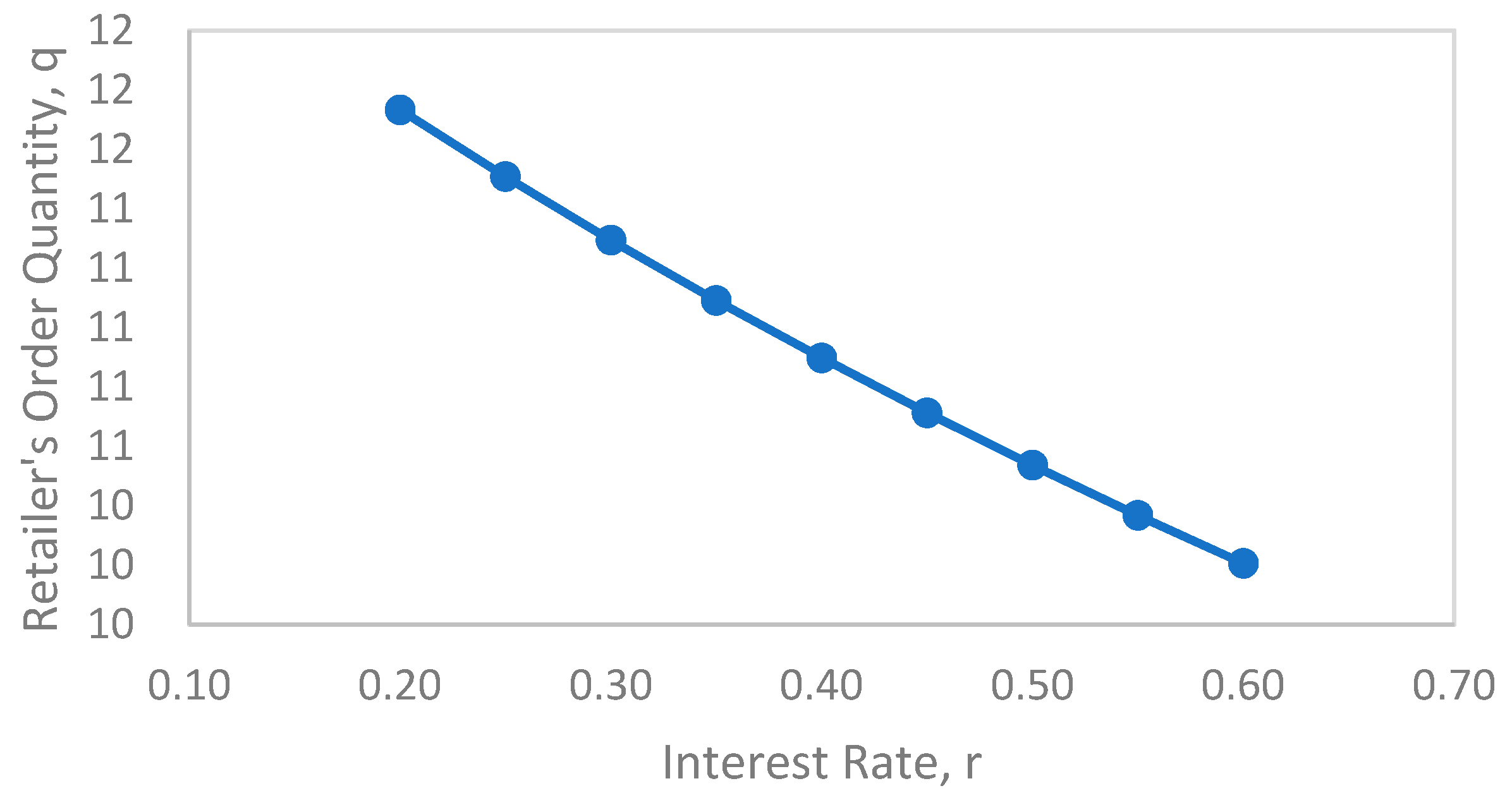
Figure 2 shows the effect of the bank’s interest rate on the retailer’s optimal order quantity. As shown in Lemma 2, it can be seen that, as the bank’s interest rate increases, the retailer’s optimal order quantity decreases.
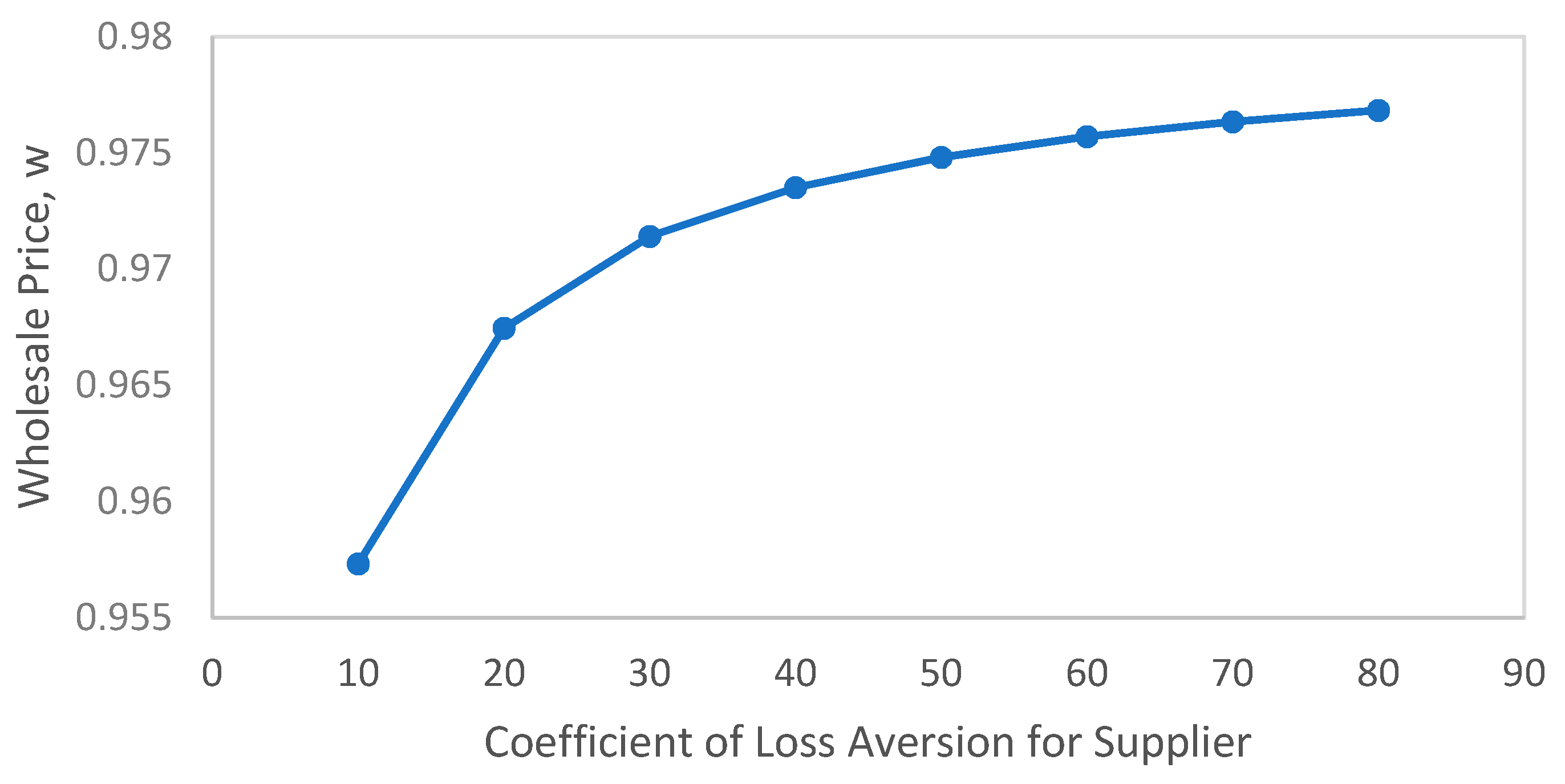
Figure 3 shows the effect of the supplier’s loss-aversion on the supplier’s wholesale price. As shown in Lemma 3, it can be seen that, as the supplier’s loss-aversion increases, the supplier’s wholesale price increases.
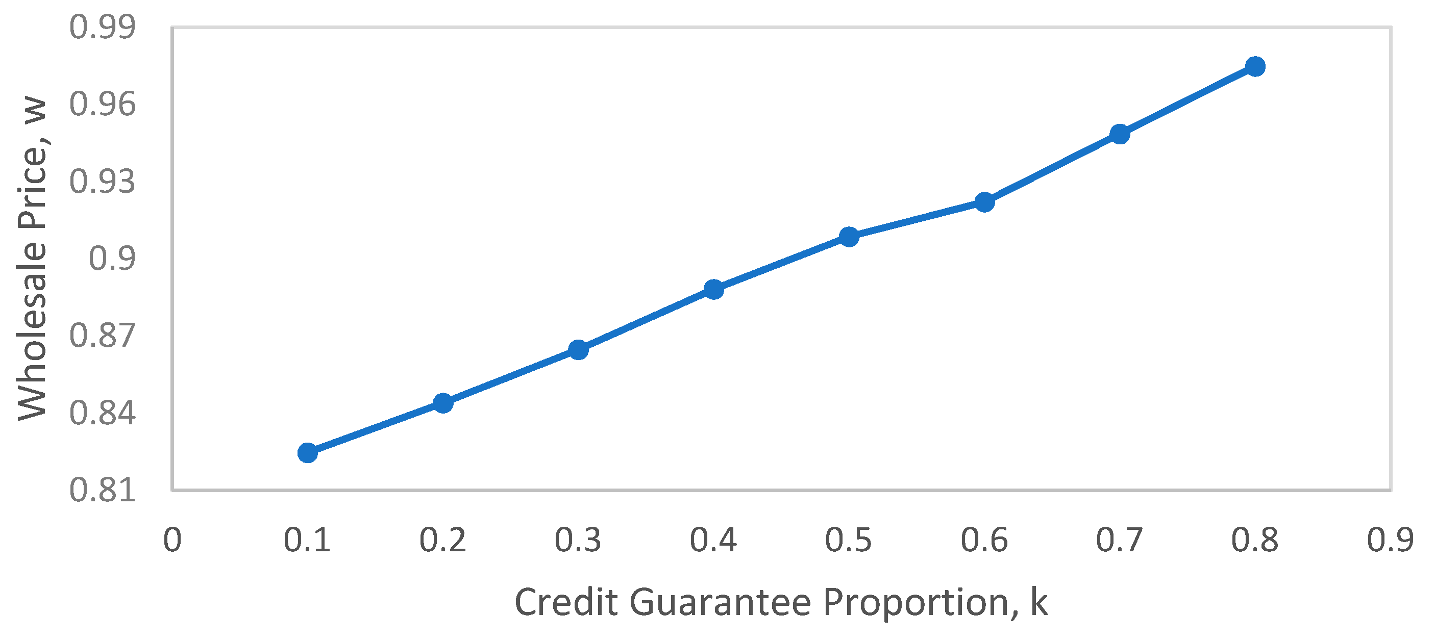
Figure 4 shows the effect of the credit guarantee on the supplier’s wholesale price. As shown in Lemma 4, it can be seen that, as the supplier’s credit guarantee increases, the supplier’s wholesale price increases.
Figure 5 shows the effect of the bank’s loss-aversion on the bank’s optimal interest rate. As shown in Lemma 6, it can be seen that, as the bank’s loss-aversion increases, the bank’s optimal interest rate increases.
5. Conclusions
This study analyses a financially constrained supply chain which consists of a financially deficient retailer, a supplier, and a bank. The bank provides a loan to the retailer considering the supplier’s credit guarantee for the retailer, which means that, if the retailer goes bankrupt after the sales season, then a pre-guaranteed proportion of the retailer’s loan is paid by the supplier instead of the retailer. Moreover, it is assumed that the supplier and the bank are loss-averse for their risk preference on the final profit. However, since the retailer’s default risk is distributed fairly evenly between the bank and the supplier by adjusting the interest rate and wholesale price, it is assumed that the retailer is risk-neutral. Then, a loss-averse preference model is formulated for the supplier and bank, in which a kinked piecewise linear and concave utility function is considered.
Although there have been studies on financially constrained supply chain problems, there have previously not been any studies on the financing strategies of loss-averse banks or the credit guarantees of loss-averse suppliers. With this loss-averse behaviour of players in the financially constrained supply chain, the optimal decision is derived for the retailer (the optimal order quantity), the supplier (the optimal wholesale price), and the bank (the optimal interest rate). Then, a sensitivity analysis is conducted to investigate how the parameters in this model affect each player’s optimal decision under different degrees of loss-aversion.
Through analytical and numerical analyses, the following results were obtained: First, in the financially constrained supply chain with bank credit and credit guarantee from the supplier, we determined the effects of the decisions of the supplier and the bank on the retailer’s optimal decision. The retailer’s optimal ordering decision is a non-increasing function of the supplier’s decision (wholesale price) and is also a non-increasing function of the bank’s decision (interest rate). The decisions of these upstream players in the supply chain can be used to adjust the retailer’s potential default risk. Second, in the financially constrained supply chain with bank credit and credit guarantee from the supplier, the larger the credit guarantee the supplier provides, the higher the wholesale price that would be charged to the retailer and the lower the interest rate that would be offered to the retailer by the bank. By this result, it can be seen that the integration of bank credit and supplier credit guarantee can be used to effectively distribute the retailer’s default risk between the bank and the supplier fairly evenly by adjusting the interest rate and wholesale price. Third, in the financially constrained supply chain, each player’s optimal decisions are indirectly affected by the degree of loss-aversion through the retailer’s possibility of bankruptcy. In addition, it is shown that the optimal wholesale price is an increasing function of the supplier’s loss-aversion and that the interest rate is an increasing function of the bank’s loss-aversion. Therefore, it can be seen that, as the degree of loss-aversion of the supplier or bank increases, the retailer’s optimal order quantity decreases. More importantly, compared with a risk-neutral supplier or risk-neutral bank, the optimal decisions for a loss-averse supplier and bank are such that both the wholesale price and the interest rate are higher and the order quantity is lower.
This study contributes to the area of financially constrained supply-chain modelling by integrating bank credit and supplier credit guarantee together with the loss-averse behaviour of players in the supply chain to investigate the effect of bank credit, credit guarantee, and loss-aversion on each player’s optimal decision.
This study investigates how the optimal decisions and loss-averse behaviour of upstream players in the supply chain influence the optimal decision of a downstream player by ignoring the goodwill loss cost, salvage cost, buyback policy, and quick response strategy, which is the limitation of this study. Therefore, in future research, this study can be extended to a model (1) that includes a buyback policy or quick response strategy, (2) in which the retailer has different risk behaviour from the risk-neutral one, and (3) which makes a demand distribution-free assumption.
Funding
This work was supported by the 2019 Hongik University Research Fund.
Conflicts of Interest
The authors declare no conflict of interest.
References
- Buzacott, J.A.; Zhang, R.Q. Inventory management with asset-based financing. Manag. Sci. 2004, 50, 1274–1292. [Google Scholar] [CrossRef]
- Kahneman, D.; Tversky, A. Prospect theory: An analysis of decision under risk. In Handbook of the Fundamentals of Financial Decision Making: Part I; World Scientific Publishing Co., Inc.: Hackensack, NJ, USA, 2013; pp. 99–127. [Google Scholar]
- Camerer, C.F. Taking Risks: The Management of Uncertainty. Adm. Sci. Q. 1988, 33, 638–640. [Google Scholar] [CrossRef]
- Arnold, J.; Minner, S. Financial and operational instruments for commodity procurement in quantity competition. Int. J. Prod. Econ. 2011, 131, 96–106. [Google Scholar] [CrossRef]
- Lee, C.H.; Rhee, B.D. Coordination contracts in the presence of positive inventory financing costs. Int. J. Prod. Econ. 2010, 124, 331–339. [Google Scholar]
- Lee, C.H.; Rhee, B.D. Trade credit for supply chain coordination. Eur. J. Oper. Res. 2011, 214, 136–146. [Google Scholar] [CrossRef]
- Lestan, Z.; Klancnik, S.; Balic, J.; Brezocnik, M. Modeling and design of experiments of laser cladding process by genetic programming and nondominated sorting. Mater. Manuf. Process. 2015, 30, 458–463. [Google Scholar] [CrossRef]
- Xu, X.; Birge, J.R. Joint Production and Financing Decisions: Modeling and Analysis. SSRN Electron. J. 2004. [Google Scholar] [CrossRef]
- Dada, M.; Hu, Q. Financing newsvendor inventory. Oper. Res. Lett. 2008, 36, 569–573. [Google Scholar] [CrossRef]
- Jing, B.; Chen, X.; Cai, G. Equilibrium financing in a distribution channel with capital constraint. Prod. Oper. Manag. 2012, 21, 1090–1101. [Google Scholar] [CrossRef]
- Kouvelis, P.; Zhao, W. Financing the newsvendor: Supplier vs. bank, and the structure of optimal trade credit contracts. Oper. Res. 2012, 60, 566–580. [Google Scholar] [CrossRef]
- Kouvelis, P.; Zhao, W. Supply chain contract design under financial constraints and bankruptcy costs. Manag. Sci. 2015, 62, 2341–2357. [Google Scholar] [CrossRef]
- Yang, S.A.; Birge, J.R. How Inventory Is (Should Be) Financed: Trade Credit in Supply Chains with Demand Uncertainty and Costs of Financial Distress. SSRN Electron. 2013. [Google Scholar] [CrossRef]
- Cressy, R.; Olofsson, C. The financial conditions for Swedish SMEs: Survey and research agenda. Small Bus. Econ. 1997, 9, 179–192. [Google Scholar] [CrossRef]
- Meyer, L.H. The present and future roles of banks in small business finance. J. Bank. Financ. 1998, 22, 1109–1116. [Google Scholar] [CrossRef]
- Bernanke, B. The federal funds rate and the channels of monetary transmission (No. w3487). Natl. Bur. Econ. Res. 1992, 84, 901–921. [Google Scholar]
- Liu, X.; Zhou, L.; Wu, Y.C. Supply chain finance in China: Business innovation and theory development. Sustainability 2015, 7, 14689–14709. [Google Scholar] [CrossRef]
- Wilner, B.S. The exploitation of relationships in financial distress: The case of trade credit. J. Financ. 2000, 55, 153–178. [Google Scholar] [CrossRef]
- Wang, C.X.; Webster, S. The loss-averse newsvendor problem. Omega 2009, 37, 93–105. [Google Scholar] [CrossRef]
- Herweg, F. The expectation-based loss-averse newsvendor. Econ. Lett. 2013, 120, 429–432. [Google Scholar] [CrossRef]
- Wang, C.X. The loss-averse newsvendor game. Int. J. Prod. Econ. 2010, 124, 448–452. [Google Scholar] [CrossRef]
- Vipin, B.; Amit, R.K. Loss aversion and rationality in the newsvendor problem under recourse option. Eur. J. Oper. Res. 2017, 261, 563–571. [Google Scholar] [CrossRef]
- Wu, M.; Bai, T.; Zhu, S.X. A loss averse competitive newsvendor problem with anchoring. Omega 2018, 81, 99–111. [Google Scholar] [CrossRef]
- Yan, N.; Liu, C.; Liu, Y.; Sun, B. Effects of risk aversion and decision preference on equilibriums in supply chain finance incorporating bank credit with credit guarantee. Appl. Stoch. Models Bus. Ind. 2017, 33, 602–625. [Google Scholar] [CrossRef]
- Zhang, Q.; Dong, M.; Luo, J.; Segerstedt, A. Supply chain coordination with trade credit and quantity discount incorporating default risk. Int. J. Prod. Econ. 2014, 153, 352–360. [Google Scholar] [CrossRef]
- Lee, J.; Lee, M.; Park, M. A newsboy model with quick response under sustainable carbon cap-n-trade. Sustainability 2018, 10, 1410. [Google Scholar] [CrossRef]
- Kim, S.; Lee, J.; Park, M. Mathematical Modelling for Risk Averse Firm Facing Loss Averse Customer’s Stochastic Uncertainty. Math. Probl. Eng. 2017, 2017. [Google Scholar] [CrossRef]
- Ren, Y.; Croson, R. Overconfidence in newsvendor orders: An experimental study. Manag. Sci. 2013, 59, 2502–2517. [Google Scholar] [CrossRef]
- Ren, Y.C.; Croson, D.; TA Croson, R. The overconfident newsvendor. J. Oper. Res. Soc. 2017, 68, 496–506. [Google Scholar] [CrossRef]
- Li, M.; Petruzzi, N.C.; Zhang, J. Overconfident competing newsvendors. Manag. Sci. 2016, 63, 2637–2646. [Google Scholar] [CrossRef]
- Sarkar, B.; Zhang, C.; Majumder, A.; Sarkar, M.; Seo, Y.W. A distribution free newsvendor model with consignment policy and retailer’s royalty reduction. Int. J. Prod. Res. 2018, 56, 5025–5044. [Google Scholar] [CrossRef]
- Sarkar, B.; Chaudhuri, K.; Moon, I. Manufacturing setup cost reduction and quality improvement for the distribution free continuous-review inventory model with a service level constraint. J. Manuf. Syst. 2015, 34, 74–82. [Google Scholar] [CrossRef]
- Moon, I.; Shin, E.; Sarkar, B. Min-max distribution free continuous-review model with a service level constraint and variable lead time. Appl. Math. Comput. 2014, 229, 310–315. [Google Scholar] [CrossRef]
- Kim, M.S.; Sarkar, B. Multi-stage cleaner production process with quality improvement and lead time dependent ordering cost. J. Clean. Prod. 2017, 144, 572–590. [Google Scholar] [CrossRef]
- Lariviere, M.A.; Porteus, E.L. Selling to the newsvendor: An analysis of price-only contracts. Manuf. Serv. Oper. Manag. 2001, 3, 293–305. [Google Scholar] [CrossRef]
- Chen, X.; Wang, A. Trade credit contract with limited liability in the supply chain with budget constraints. Ann. Oper. Res. 2012, 196, 153–165. [Google Scholar] [CrossRef]
- Gill, P.; Abend, J. Wal-Mart: The supply chain heavyweight champ. Supply Chain Manag. Rev. 1997, 1, 8–16. [Google Scholar]
- Clark, T.H.; McKenney, J.L. Campbell Soup Company: A leader in continuous replenishment innovations. Harv. Bus. Sch. Case 1994, 9, 195124. [Google Scholar]
- Hammond, J.H. Quick Response in Manufacturing-retail Channels. In Globalization, Technology, and Competition: The Fusion of Computers and Telecommunications in the 1990s; Bradley, S.P., Hausman, J.A., Nolan, R.L., Eds.; Harvard Business School Press: Boston, MA, USA, 1993; pp. 185–214. [Google Scholar]
- Lee, H.L.; So, K.C.; Tang, C.S. The value of information sharing in a two-level supply chain. Manag. Sci. 2000, 46, 626–643. [Google Scholar] [CrossRef]
- Chen, X. A model of trade credit in a capital-constrained distribution channel. Int. J. Prod. Econ. 2015, 159, 347–357. [Google Scholar] [CrossRef]
Figure 1.
Retailer’s optimal order quantity vs. supplier’s wholesale price.

Figure 2.
Retailer’s optimal order quantity vs. the bank’s interest rate.

Figure 3.
Optimal wholesale price vs. supplier’s coefficient of loss-aversion.

Figure 4.
Optimal wholesale price vs. credit guarantee proportion (k).

Figure 5.
Bank’s optimal interest rate vs. bank’s coefficient of loss-aversion.

© 2019 by the author. Licensee MDPI, Basel, Switzerland. This article is an open access article distributed under the terms and conditions of the Creative Commons Attribution (CC BY) license (http://creativecommons.org/licenses/by/4.0/).
Share and Cite
MDPI and ACS Style
Lee, J. Impact of Loss-Aversion on a Financially-Constrained Supply Chain. Sustainability 2019, 11, 2680. https://doi.org/10.3390/su11092680
AMA Style
Lee J. Impact of Loss-Aversion on a Financially-Constrained Supply Chain. Sustainability. 2019; 11(9):2680. https://doi.org/10.3390/su11092680
Chicago/Turabian StyleLee, Jinpyo. 2019. "Impact of Loss-Aversion on a Financially-Constrained Supply Chain" Sustainability 11, no. 9: 2680. https://doi.org/10.3390/su11092680
Note that from the first issue of 2016, this journal uses article numbers instead of page numbers. See further details here.