Response of Water Quality to Landscape Patterns in an Urbanized Watershed in Hangzhou, China

1
Institute of Remote Sensing and Earth Sciences (IRSE), College of Science, Hangzhou Normal University, Hangzhou 311121, China
2
Zhejiang Provincial Key Laboratory of Urban Wetlands and Regional Change, Hangzhou 311121, China
3
College of Geomatics & Municipal Engineering, Zhejiang University of Water Resources and Electric Power, Hangzhou 310018, China
4
Department of Forestry and Natural Resources, Purdue University, West Lafayette, IN 47907, USA
*
Author to whom correspondence should be addressed.
Sustainability 2020, 12(14), 5500; https://doi.org/10.3390/su12145500
Submission received: 11 April 2020
/
Revised: 3 June 2020
/
Accepted: 23 June 2020
/
Published: 8 July 2020
(This article belongs to the Section Environmental Sustainability and Applications)
Abstract
:Intense human activities and drastic land use changes in rapidly urbanized areas may cause serious water quality degradation. In this study, we explored the effects of land use on water quality from a landscape perspective. We took a rapidly urbanized area in Hangzhou City, China, as a case study, and collected stream water quality data and algae biomass in a field campaign. The results showed that built-up lands had negative effects on water quality and were the primary cause of stream water pollution. The concentration of total phosphorus significantly correlated with the areas of residential, industrial, road, and urban greenspace, and the concentration of chlorophyll a also significantly correlated with the areas of these land uses, except residential land. At a landscape level, the correlation analysis showed that the landscape indices, e.g., dominance, shape complexity, fragmentation, aggregation, and diversity, all had significant correlations with water quality parameters. From the perspective of land use, the redundancy analysis results showed that the percentages of variation in water quality explained by the built-up, forest and wetland, cropland, and bareland decreased in turn. The spatial composition of the built-up lands was the main factor causing stream water pollution, while the shape complexities of the forest and wetland patches were negatively correlated with stream water pollution.
1. Introduction
Land use change is one of the key driving forces of global change and terrestrial environmental changes [1,2,3]. Land use may exert considerable influence on stream environments by altering multiple ecological processes, e.g., hydrological cycle, soil erosion, and nutrient migration and transformation [4,5]. Point and non-point source pollutants are the main contributors to stream water pollution. Non-point source pollution still affects stream water quality in developed regions where the point source pollutions are usually under effective control, and almost all non-point source pollutions are closely related to land use change [6,7,8,9,10,11,12]. At the watershed scale, the influence of land use on stream water quality is of particular interest [13,14]. The water quality in a particular watershed is determined by multiple environmental factors, as the migration and transformation of pollutants at the land surface are closely associated with the local environment (e.g., vegetation and soil) and human activities (e.g., urbanization). In this process, the landscape pattern is a critical factor to understand the spatial variation of stream water quality [15,16].
The relationship between landscape patterns and ecological processes is one of the key issues in landscape ecology [17,18,19]. Two kinds of study strategies, i.e., the composition and structure of landscape perspectives, respectively, are commonly applied to study the relationships between landscape pattern and stream water quality; the former focuses on the correlation between land use pattern and water quality [20,21], while the latter emphasizes the influence of landscape spatial structure of land use on water quality [22,23,24,25]. Due to the limited understanding of nutrient transport process and mechanism in soil and soil interface, model simulations are mainly used to estimate the non-point source pollution and nutrient transport in stream water, while studies about the influence of land use pattern on water quality parameters, e.g., the total nitrogen and total phosphorus, mainly rely on statistical methods [26,27,28].
Rapidly urbanized areas are characterized by intense human activities, drastic land use changes, and, especially, serious water quality degradation [29,30]. Numerous studies about the relationship between land use and water quality in agricultural and forestry watersheds can be found in the literature, but studies about the response of water quality to landscape patterns in rapidly urbanized watersheds are still uncommon [31,32,33]. Nevertheless, it has been suggested that in rapidly urbanized areas, for example, the quickly expanded megacities in China, point source pollution control measures are not enough to solve water deterioration, as non-point source pollution is now one of the leading sources of water pollution in these regions.
Non-point source pollution is closely related to land use, and the landscape pattern is a critical linkage between human activities and water quality in urbanized areas [34,35,36]. The fragmentation of landscape generally increased with urbanization, that is, the original homogeneous, intact, and continuous natural landscape shifts to be heterogeneous and discontinuous with mixed patches [37,38]. Most common landscape pattern metrics used in this field are compositional; however, the spatial structure indicators used to quantify the complexity, fragmentation, agglomeration, connectivity, and diversity of landscape were not yet fully studied [39,40,41]. We argue that these kinds of landscape metrics might be useful to integrate the migration and accumulation of pollutants among heterogeneous patches and should be considered in the study of the relationship between landscape pattern and water quality. Therefore, our objectives were to quantitatively address the following questions: (1) For typically urbanized watershed, how does the landscape pattern affect the water quality of urban streams? And (2) what are the most influential landscape metrics to be considered in management options for water quality in rapidly urbanized areas? We selected one quickly urbanized region in the west of Hangzhou City, one of the megacities in China, as the study area. Data on water quality and algae biomass were collected in field campaigns, and the land use data were obtained from high-resolution remote sensing. The relationship between landscape pattern and water quality parameters at the watershed scale was analyzed from the perspective of the spatial composition of land use.
2. Materials and Methods
2.1. Study Area
Hangzhou City is located south of the Yangtze River Delta in China. The study area, characterized by piedmont watersheds and large areas of wetlands (Wuchang and Hemu) with densely distributed stream network, is at the west of Hangzhou (Figure 1). During the past decade, the study area has experienced intense urbanization with large scale land use transformation from cropland and wetland to built-up lands.
2.2. Land Use Classification
A two-level classification system was adapted from the Chinese Standard of Land Use Classification [42]. We classified the land use in the study area into five Level I classes, i.e., Cropland (1), Forest (2), Water (3), Built-up (4), and Bareland (5), and 12 Level II classes, i.e., Cropland (11), Forest (21), River (31), Pond (32), Residential (41), Industrial (42), Commercial (43), Public management and service (44), Urban greenspace (45), Road (46), Under construction (47), and Bareland (51), respectively. The land use information was extracted from one cloudless SPOT 6 image obtained on October 26, 2014. The multispectral and panchromatic bands of the SPOT image were fused to get a 1.5 m resolution image using the Gram–Schmidt method [43]. The SPOT image was radiometrically and atmospherically corrected, and the accuracy of geometric correction was under 0.5 pixels. The Level I land use classes were extracted by supervised classification method with a total accuracy of 91.49% and that kappa coefficient of 0.88, and then further subclassified into corresponding Level II classes using visual interpretation with the aid of ancillary data, e.g., ASTER DEM, field survey data, and Google Earth satellite images [44] (Figure 2). The classification accuracy was assessed by stratified random sampling with reference to ground-truth data collected through field survey. The assessment results showed that the overall accuracy of land use classification was 93.23% and that the kappa coefficient was 0.92.
2.3. Watershed Delineation
A fine delineation of the watershed is crucial in evaluating the influence of land use on water quality in relatively small areas. The commonly used watershed delineation algorithms, e.g., D8 [45], burn-in [46], DEMOM [47], and Dinf [48], work well in plain areas with low impact of human activities. However, the road partition, river embankments, and buildings in complex urban areas could alter the original runoff directions [49]. One feasible solution to improve the accuracy of watershed delineation, in this case, is to combine these terrain features into the Digital Elevation Model (DEM) [50]. Considering that the study area is composed of piedmont plains with dense stream networks and complex built-up land uses, we combined the land use map and adjusted the DEM before watershed delineation using the D8 algorithm (Figure 3). The primary goal of this operation was to adjust the elevation values of the terrestrial features, e.g., buildings, ditch, and greenspace, to more closely reflect the urban surface morphology, and, especially, the surface runoff direction, as the buildings will block natural runoff while the ditches and greenspace could divert and absorb surface runoff [51,52,53].
2.4. Water Sampling
Based on the watershed division and the spatial distribution of the stream network and land use, sampling points were selected to evenly cover each sub-basin. In total 19 sampling points were selected near the outlet of each sub-basin. The water sampling was conducted within one week, when the stream flow was relatively stable during the local high water period in June 2014 (Figure 3). Aside from the total nitrogen (TN) and total phosphorus (TP), we also measured the concentration of chlorophyll a (TChla), including chlorophyll a concentration of Cyanophyta (ChlaCyan), chlorophyll a concentration of Chlorophyta (ChlaChlo), and chlorophyll a concentration of Bacillariophyta and Dinophyta (ChlaBaci-Dino), using a four-wavelength-excitation chlorophyll fluorometer (PHYTO-PAM Fa. Walz, Effeltrich, Germany). The water samples were collected 0.3–0.5 m below the water surface from the middle of the stream with a 250 mL organic glass hydrophore, and three parallel samples were collected at each sampling site to avoid accidental errors. The samples were kept in iceboxes during transport to the laboratory. The TP and TN were determined using the alkaline potassium persulfate digestion UV spectrophotometric method (GB11893-89, China National Standards) and the ammonium molybdate spectrophotometric method (GB11894-89, China National Standards), respectively. According to the Environmental Quality Standards for Surface Water (EQSSW) (GB3838-2002, State Environmental Protection Administration of China), the water quality could be classified into five classes by a series water quality parameters, including TN and TP, and the higher the class, the worse the water quality.
2.5. Landscape Metrics
There are numerous landscape metrics that quantitatively represent the spatial composition of a particular landscape pattern [20,22,23,54,55,56]. In this study, we used five categories of metrics, i.e., area-edge, subdivision, contagion/intersection, diversity, and shape, to quantify the landscape pattern and explore the corresponding associations with water quality parameters (Table 1). The landscape metrics at the landscape and class levels were analyzed by the software FRAGSTATS 4.1.
2.6. Statistical Analysis
The Spearman rank correlation was used to analyze the relationships between land use and water quality parameters. We used the Spearman rank correlation coefficient due to the nonparametric nature of the data, as the Shapiro–Wilk test of normality showed that most of the water quality and land use data did not follow normal distribution [57]. The multiple linear regression (MLR) was performed to evaluate the relationships between response (i.e., single water quality parameter) and predictors (i.e., land use metrics) after Spearman rank correlation analysis. To reduce the redundancy associated with the correlated variables, a stepwise regression approach based on the p values was chosen to eliminate insignificant predictor variables from the MLR models. The dependent and predictor variables were log-transformed to reduce the influence of the asymmetric distribution of the data [24,58]. The regression analyses were carried out with SPSS 16.0.
The constrained ordination methods, e.g., redundancy analysis (RDA) and canonical correspondence analysis (CCA), could well extract the variation in response variables that can be explained by a set of explanatory variables and have been widely used to analyze the relationships between land use pattern and water quality parameters [59,60,61,62]. The detrended correspondence analysis (DCA) showed that the maximum length of the gradient of the water quality data was less than three standard deviations, suggesting that the relationship between water quality and landscape metrics could be either linear or unimodal. Therefore, RDA was used to explore the relationship between water quality and landscape pattern parameters. The statistically significant landscape metrics in RDA were identified using a Monte Carlo permutation test (499 non-restrictive screening cycles) [63]. To simplify the interpretation of RDA results about the relationships between landscape pattern and water quality parameters, we further categorized the Level I land use classes (see Section 2.2) into four classes, i.e., cropland, forest, and wetland (by merging the forest and water classes), built-up, and bareland, from a functional perspective. The RDA was performed using the CANOCO 4.5 program.
3. Results
3.1. Land Use Structure and Water Quality
Land use in each catchment is shown in Figure 4. The built-up land area accounted for nearly 50% of the whole study area. The areas of forest, cropland, and residential land covered 18.84%, 16.42%, and 16.42% of the study area, respectively. The areas of under construction, industrial use, and bareland occupied 9.42%, 7.19%, and 6.92% respectively, followed by the roads (5.53%), urban greenspaces (5.34%), ponds (4.99%), and the river (3.87%). The areas of public management and service, and commercial land, were the smallest with percentages of 3.20% and 1.86%, respectively.
The statistics of the water quality and the corresponding spatial distributions are shown in Table 2 and Figure 5. The average concentrations of TN and TP were 6.54 mg/L and 0.62 mg/L, respectively, both exceeding the thresholds of TN and TP, i.e., 2.0 mg/L and 0.4 mg/L, of Class V in EQSSW. The TN concentrations at 16% and 84% sampling sites were Class V and beyond, respectively. The TP concentrations at 11%, 21%, 11%, and 53% sampling points were Class III, IV, V, and beyond, respectively; only No. 19 sampling point was Class II.
The average concentrations of ChlaCyan, ChlaChlo, and ChlaBaci-Dino were 9.90 µg/L, 68.44 µg/L, and 24.15 µg/L, respectively. In 63% of the sampling sites, no ChlaCyan were detected. The average TChla was 94.08 µg/L, much higher than the OECD eutrophication evaluation criteria [64].
The correlation analysis showed that TN was positively correlated with TP; TChla was positively correlated with TP; and ChlaChlo was positively correlated with TN, TP, and Tchla, respectively (Table 3).
3.2. Relationships Between Land Use Area and Water Quality
The correlation analysis between stream water quality and land use areas showed TP was positively correlated with the areas of residential, industrial, road, and urban greenspace (Figure 6). The ChlaBaci-Dino, ChlaChlo, and TChla were positively correlated with the areas of river, pond, and bareland; the ChlaChlo was positively correlated with the areas of road and urban greenspace; and the TChla was positively correlated with areas of road, urban greenspace, and industrial. Additionally, there were no statistically significant correlations between water quality parameters and the areas of cropland, commercial, public management and service, and under construction.
The stepwise multiple linear regression between water quality parameters and land use areas (Table 4) showed that industrial land was the dominant predictor of both TP and TChla concentrations, while bareland was the dominant predictor of algae biomass.
3.3. Relationships Between Landscape Pattern and Water Quality
3.3.1. Land Use Pattern—Water Quality Relationships at Landscape Level
The correlation analysis between landscape pattern and water quality parameters showed that (Figure 7) the landscape metrics, e.g., dominance (LPI), complexity (SHAPE, FRAC, PARA, and LSI), fragmentation (TE, NP, and DIVISION), aggregation and connectedness (CONTAG, IJI, and CONTIG), and diversity (PR and SHDI), all had significant correlations with water quality parameters. TP, TChla, and ChlaChlo, compared with TN, ChlaCyan, and ChlaBaci-Dino, were much more sensitive to landscape metrics and negatively correlated with LPI, FRAC, and CONTAG, but positively correlated with SHDI. The ChlaBaci-Dino were only negatively correlated with SHAPE and FRAC, two landscape metrics related to the shape of landscape patches. The ChlaCyan showed no significant correlations with the landscape metrics, so no further analysis of this parameter was carried out.
The relationships between landscape pattern metrics and water quality parameters were also analyzed by the stepwise multiple linear regression modeling. As shown in Table 5, the PARA was the dominant predictor both for TN and TP; while SHDI was the dominant predictor both for TChla and ChlaChlo, and SHAPE was the dominant predictor for ChlaBaci-Dino.
3.3.2. Land Use Pattern—Water Quality Relationships at Class Level
For the four land use classes, there were 2, 5, 7, and 5 explanatory variables with statistically significant relationships with water quality parameters, respectively (Table 6). The total explained variations in water quality were 37.9%, 54.6%, 71.4%, and 35.9%, respectively, and more than 90% variations in water quality parameters could be explained by the first two axes. The built-up land use had the highest total explained variation. For all land use types, the total explained variations in water quality were 84.1%.
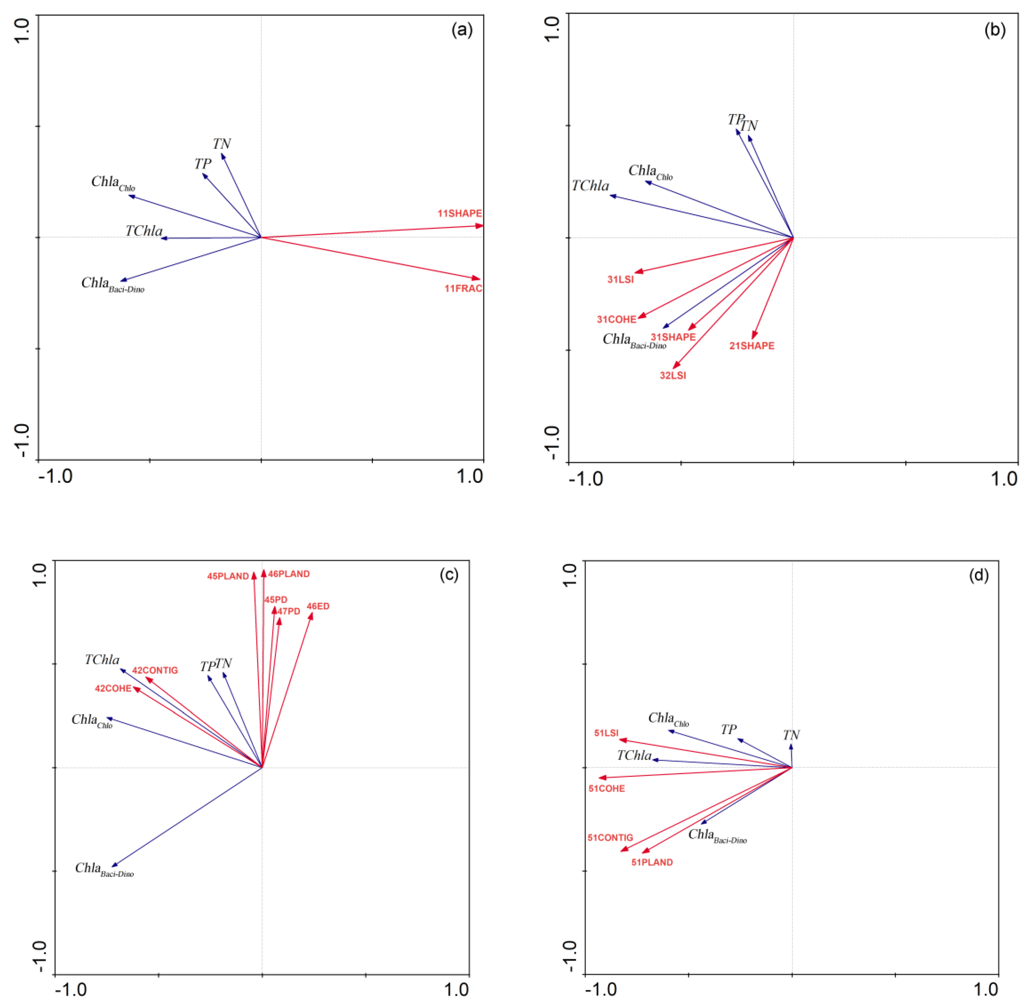
The RDA showed that the landscape patterns had different influences on water quality parameters (Figure 8). The TN and TP were negatively correlated with the landscape shape metrics of the cropland and forest. In addition, the ordination also showed that TN and TP were affected by the landscape patterns of the built-up land uses. For example, TN and TP were positively correlated with PLANDs of the road and urban greenspace, PDs of the urban greenspace and under construction, and the ED of the road, as well as the COHE and CONTIG of the industrial land. The ChlaChlo and TChla showed similar responses to the landscape pattern; these two parameters were negatively correlated with SHAPE and FRAC metrics of cropland, and positively correlated with LSI, COHE, and CONTIG metrics of bareland and the COHE and CONTIG metrics of industrial land. The ChlaBaci-Dino showed significant correlations with the landscape metrics related to the complexity of the forest and wetland patches; for example, the ChlaBaci-Dino was positively correlated with the SHAPE and LSI metrics of the river, as well as the LSI of the pond and the SHAPE of the forest.
To be specific, water pollution, in terms of TN and TP, was positively correlated with the following landscape metrics, i.e., the connectedness of the industrial land, the dominance and fragmentation of the road and urban greenspace, and the fragmentation of the under construction land. On the contrary, the complexities of the cropland and forest patches were negatively correlated with TN and TP. The algae biomass, especially the ChlaBaci-Dino, was positively correlated with the complexities of the river as well as the pond patches, and the connectedness of the river. The complexity of the bareland patch was also a positive indicator of the TChla.
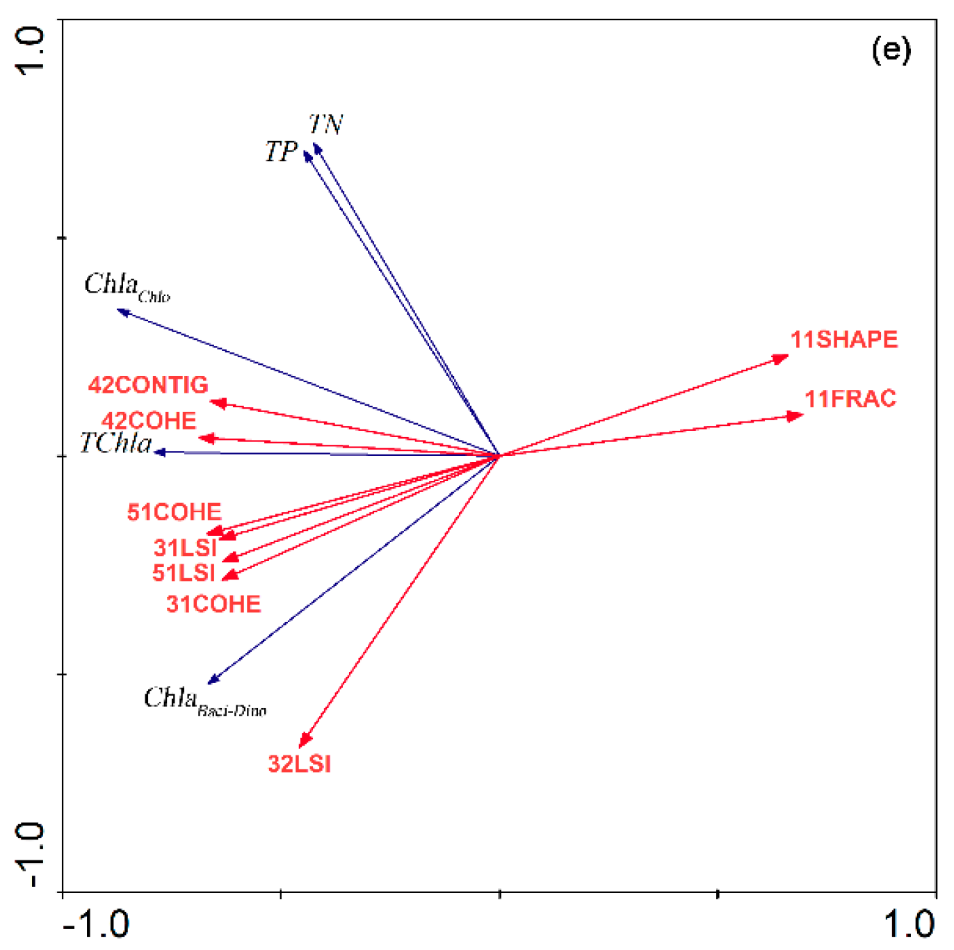
By using both types of land use metrics, RDA showed that CONTIG and COHESION of the industrial land, COHESION and LSI of the bareland, COHESION and LSI of the river, LSI of the lake and pond, and SHAPE and FRAC of the cropland were the main factors dominating the variation in water quality.
4. Discussion
4.1. Water Pollution in Urbanized Watershed
The stream water in the study area was eutrophic with serious nitrogen and phosphorus pollution and high algae biomass (Table 2). The percentage of impervious surface is an indicator that could well represent the intensity of urbanization, including its spatial expansion. Of all the influential factors in terms of water quality in urban area, stream water quality, and aquatic ecosystems could be damaged if the ratio of impervious surface reaches 10–15% in a specific watershed [65,66,67,68]. For our case, the percentage of the impervious surface was over 50%, much higher than the threshold mentioned above (Figure 4).
The built-up lands were important factors influencing water quality in the study area. For example, the TP was positively correlated with the areas of residential, industrial, road, and urban greenspace, and the TChla was also positively correlated with the areas of industrial, road, and urban greenspace. The TN was positively correlated with the areas of all the built-up lands, although none were statistically significant (Figure 6). The increased built-up areas in urban area could result in a considerable increase of non-point source pollutants by precipitation runoff [69,70,71].
The biomass of ChlaChlo was positively correlated with TN and TP, but the correlations between ChlaBaci-Dino and TN as well as TP were not statistically significant (Table 3). The TChla, ChlaChlo, and ChlaBaci-Dino positively correlated with the areas of the pond and river (Figure 6). In addition to the absolute concentration of TN and TP, the growth of algae is also affected by factors like the ratio of nitrogen and phosphorus, water pH, and dissolved oxygen [72,73], and, therefore, the community structure of algae might not be simply explained by the nutrient concentrations in stream water alone. Urban greenspace, contrary to common sense, was positively correlated with ChlaChlo, TChla, as well as TP. We suggested that this phenomenon might be due to the urban greenspace in rapidly urbanized areas being not yet fully functional ecosystems and, additionally, the urban greenspace was mainly concentrated along with the road and was a major sink of vehicle emissions.
4.2. Influence of Landscape Patterns on Water Quality
During the urbanization, the landscape usually shows a trend of fragmentation, decentralization, and diversification with decreased complexity of the patch shape as the dominant landscape of the cropland or forest are replaced by various built-up land uses [25,74,75,76]. We found that the dominance, fragmentation, complexity, and diversity of the landscape at the catchment scale were closely related to stream water quality (Figure 7).
It is hard to quantify the response of water quality to specific land use status without the corresponding landscape pattern of the target land use [56,77]. Indeed, different kinds of land uses had varied explanatory abilities to water quality. The landscape metrics of the built-up land had the highest explanatory ability, followed by the forest, water, cropland, and bareland (Table 6). The results further showed that the spatial composition of the built-up land and the complexities of the forest, water, and cropland patches had close relationships with stream water quality. To be specific, the TN and TP were positively correlated with the connectedness of the industrial land, road area, and the fragmentations of urban greenspace and under construction lands were positive indicators of the TN and TP in the stream water in this study area.
There are numerous studies about the relationships between the dominance and fragmentation of the built-up land and water quality [22,24,78], but a more detailed classification of the built-up land is still needed to more accurately locate the problem. In this study, we classified the built-up land into residential, industrial, commercial, public management and service, urban greenspace, road, and under construction, and quantitatively analyzed the relationship between stream water quality and multiple landscape pattern metrics of all the built-up land uses using RDA. We found that a detailed classification of the built-up land could help more accurately identify the most influential land uses and the corresponding landscape patterns on water quality. For example, we found that the connectedness of the industrial land, dominances and fragmentations of the road and urban greenspace, and the fragmentation of the under construction land were correlated with the concentrations of TN and TP in the stream water. By identifying the influential land uses and the corresponding landscape pattern metrics, it might be possible to artificially influence water quality by optimizing the composition and spatial pattern of the specific land uses [79,80].
The forest may have a direct impact on the hydrological status of a specific catchment. The area, aggregation, and connectedness of the forest landscape were usually positively correlated with the abilities of fixation and retention of water pollutants, as well as the purification of surface runoff [81,82]. In this case, we found that the increased complexities of the forest and cropland landscapes were associated with the decreased TN and TP in the stream water, and this finding might be of interest to the forest or cropland planning practitioners.
4.3. Limits and Future Work
For studies about the relationship between water quality and land use/land cover changes at the medium or large watershed scales, series land use data and long-term water quality data are usually a prerequisite [14,71]. However, the hydrological stations and long-term water quality data at urban watersheds are usually quite limited. This study analyzed the response of stream water quality to the catchment landscape pattern using data collected during the high water period, but its applicability during the dry season or the flat water period still needs verification. Additionally, the land use status and water quality are constantly changing during the urbanization process [70,83], and it would be expected that regular monitoring of the land use change and water quality in urban areas could provide more effective guidance in urban land use planning and water environment management.
We showed the ability of landscape metrics to explain the variation of specific water quality parameters. However, many of the studies about the relationship between water quality and land use are case-specific and the selection of landscape metrics remains more or less subjective [84,85,86], so we suggested that it would be helpful to establish a common set of landscape metrics with clear ecological significance to improve the comparability across similar studies.
5. Conclusions
The feedback of water quality on landscape patterns was analyzed at the catchment scale in a typical rapidly urbanized area with a dense stream network. The stream water in the study area was characterized by eutrophic water with serious nitrogen and phosphorus pollution and high algae biomass. The built-up lands showed negative effects on water quality. The TP was positively correlated with areas of residential, industrial, road, and urban greenspace; except residential land, the TChla had similar statistical correlations with the areas of the other three land uses.
At the landscape level, the TP, ChlaChlo, and TChla were positively correlated with the decreased landscape dominance and shape complexity, and the increased landscape fragmentation and dispersity. At the class level, the percentages of the variation in water quality explained by the built-up land, forest and wetland, cropland, and bareland decreased in turn. The spatial composition of the built-up lands was the main factor causing stream water pollution, while the shape complexities of forest and wetland patches were negatively correlated with stream water pollution.
We suggested that, in order to improve water quality during rapid urbanization, it might be necessary to avoid the uncontrolled sprawl of construction land, especially of industrial land, and the excessive dispersion and fragmentation of farmland, and to improve the connectivity of rivers and the complexities of forests and wetlands.
Author Contributions
Y.S. and X.S. conceived and designed the framework of the research structure. Y.S., X.S. and G.S. contributed to the data analysis, interpretation, and manuscript writing. Y.S., X.S. and G.S. All authors have read and agreed to the published version of the manuscript.
Funding
This research was funded by the Natural Science Foundation of Zhejiang Province, China (grant number: LQ13C030007), Entrepreneurship and Innovation Project for High-level Overseas Returnees in Hangzhou City in 2019, and Science and Technology Project of the Water Resources Department of Zhejiang Province (grant number: RC1810).
Conflicts of Interest
The authors declare no conflict of interest.
References
- Grimm, N.B.; Faeth, S.H.; Golubiewski, N.E.; Redman, C.L.; Wu, J.; Bai, X.; Briggs, J.M. Global change and the ecology of cities. Science 2008, 319, 756–760. [Google Scholar] [CrossRef] [PubMed] [Green Version]
- Pielke, R.A. Land use and climate change. Science 2005, 310, 1625–1626. [Google Scholar] [CrossRef] [PubMed] [Green Version]
- Song, W.; Deng, X. Land-use/land-cover change and ecosystem service provision in China. Sci. Total Environ. 2017, 576, 705–719. [Google Scholar] [CrossRef]
- Guzha, A.; Rufino, M.C.; Okoth, S.; Jacobs, S.; Nóbrega, R. Impacts of land use and land cover change on surface runoff, discharge and low flows: Evidence from East Africa. J. Hydrol. Reg. Stud. 2018, 15, 49–67. [Google Scholar] [CrossRef]
- Borrelli, P.; Robinson, D.A.; Fleischer, L.R.; Lugato, E.; Ballabio, C.; Alewell, C.; Meusburger, K.; Modugno, S.; Schütt, B.; Ferro, V. An assessment of the global impact of 21st century land use change on soil erosion. Nat. Commun. 2017, 8, 1–13. [Google Scholar] [CrossRef] [Green Version]
- Charbonneau, R.; Kondolf, G. Land use change in California, USA: Nonpoint source water quality impacts. Environ. Manag. 1993, 17, 453–460. [Google Scholar] [CrossRef]
- Brett, M.T.; Arhonditsis, G.B.; Mueller, S.E.; Hartley, D.M.; Frodge, J.D.; Funke, D.E. Non-point-source impacts on stream nutrient concentrations along a forest to urban gradient. Environ. Manag. 2005, 35, 330–342. [Google Scholar] [CrossRef] [PubMed]
- Abdulkareem, J.H.; Sulaiman, W.N.A.; Pradhan, B.; Jamil, N.R. Long-term hydrologic impact assessment of non-point source pollution measured through Land Use/Land Cover (LULC) changes in a tropical complex catchment. Earth Syst. Environ. 2018, 2, 67–84. [Google Scholar] [CrossRef]
- Basnyat, P.; Teeter, L.D.; Lockaby, B.G.; Flynn, K.M. The use of remote sensing and GIS in watershed level analyses of non-point source pollution problems. For. Ecol. Manag. 2000, 128, 65–73. [Google Scholar] [CrossRef]
- Tong, S.T.; Chen, W. Modeling the relationship between land use and surface water quality. J. Environ. Manag. 2002, 66, 377–393. [Google Scholar] [CrossRef]
- White, M.J.; Storm, D.E.; Busteed, P.R.; Stoodley, S.H.; Phillips, S.J. Evaluating nonpoint source critical source area contributions at the watershed scale. J. Environ. Qual. 2009, 38, 1654–1663. [Google Scholar] [CrossRef] [PubMed]
- Tu, M.-C.; Smith, P. Modeling pollutant buildup and washoff parameters for SWMM based on land use in a semiarid urban watershed. Water Air Soil Pollut. 2018, 229, 121. [Google Scholar] [CrossRef]
- Welde, K.; Gebremariam, B. Effect of land use land cover dynamics on hydrological response of watershed: Case study of Tekeze Dam watershed, northern Ethiopia. Int. Soil Water Conserv. Res. 2017, 5, 1–16. [Google Scholar] [CrossRef]
- Turner, R.E.; Rabalais, N.N. Linking landscape and water quality in the Mississippi River Basin for 200 years. BioScience 2003, 53, 563–572. [Google Scholar] [CrossRef]
- McGrane, S.J. Impacts of urbanisation on hydrological and water quality dynamics, and urban water management: A review. Hydrol. Sci. J. 2016, 61, 2295–2311. [Google Scholar] [CrossRef]
- Schröder, B. Pattern, Process, and Function in Landscape Ecology and Catchment Hydrology? How Can Quantitative Landscape Ecology Support Predictions in Ungauged Basins? Hydrol. Earth Syst. Sci. 2006, 10, 967–979. [Google Scholar] [CrossRef] [Green Version]
- Turner, M.G. Landscape ecology: The effect of pattern on process. Annu. Rev. Ecol. Syst. 1989, 20, 171–197. [Google Scholar] [CrossRef]
- Ward, J.; Malard, F.; Tockner, K. Landscape ecology: A framework for integrating pattern and process in river corridors. Landsc. Ecol. 2002, 17, 35–45. [Google Scholar] [CrossRef]
- Arroyo-Rodríguez, V.; Melo, F.P.; Martínez-Ramos, M.; Bongers, F.; Chazdon, R.L.; Meave, J.A.; Norden, N.; Santos, B.A.; Leal, I.R.; Tabarelli, M. Multiple successional pathways in human-modified tropical landscapes: New insights from forest succession, forest fragmentation and landscape ecology research. Biol. Rev. 2017, 92, 326–340. [Google Scholar] [CrossRef]
- Alberti, M.; Booth, D.; Hill, K.; Coburn, B.; Avolio, C.; Coe, S.; Spirandelli, D. The impact of urban patterns on aquatic ecosystems: An empirical analysis in Puget lowland sub-basins. Landsc. Urban Plan. 2007, 80, 345–361. [Google Scholar] [CrossRef]
- Johnson, L.; Richards, C.; Host, G.; Arthur, J. Landscape influences on water chemistry in Midwestern stream ecosystems. Freshw. Biol. 1997, 37, 193–208. [Google Scholar] [CrossRef]
- Lee, S.-W.; Hwang, S.-J.; Lee, S.-B.; Hwang, H.-S.; Sung, H.-C. Landscape ecological approach to the relationships of land use patterns in watersheds to water quality characteristics. Landsc. Urban Plan. 2009, 92, 80–89. [Google Scholar] [CrossRef]
- Uuemaa, E.; Roosaare, J.; Mander, Ü. Landscape metrics as indicators of river water quality at catchment scale. Hydrol. Res. 2007, 38, 125–138. [Google Scholar] [CrossRef]
- Ding, J.; Jiang, Y.; Liu, Q.; Hou, Z.; Liao, J.; Fu, L.; Peng, Q. Influences of the land use pattern on water quality in low-order streams of the Dongjiang River basin, China: A multi-scale analysis. Sci. Total Environ. 2016, 551, 205–216. [Google Scholar] [CrossRef] [PubMed]
- Shi, P.; Zhang, Y.; Li, Z.; Li, P.; Xu, G. Influence of land use and land cover patterns on seasonal water quality at multi-spatial scales. Catena 2017, 151, 182–190. [Google Scholar] [CrossRef]
- Borah, D.; Bera, M. Watershed-scale hydrologic and nonpoint-source pollution models: Review of mathematical bases. Trans. ASAE 2003, 46, 1553. [Google Scholar] [CrossRef] [Green Version]
- Xiang, C.; Wang, Y.; Liu, H. A scientometrics review on nonpoint source pollution research. Ecol. Eng. 2017, 99, 400–408. [Google Scholar] [CrossRef]
- Fraga, I.; Charters, F.; O’Sullivan, A.; Cochrane, T. A novel modelling framework to prioritize estimation of non-point source pollution parameters for quantifying pollutant origin and discharge in urban catchments. J. Environ. Manag. 2016, 167, 75–84. [Google Scholar] [CrossRef]
- Arnold, C.L., Jr.; Gibbons, C.J. Impervious surface coverage: The emergence of a key environmental indicator. J. Am. Plan. Assoc. 1996, 62, 243–258. [Google Scholar] [CrossRef]
- Giri, S.; Qiu, Z. Understanding the relationship of land uses and water quality in Twenty First Century: A review. J. Environ. Manag. 2016, 173, 41–48. [Google Scholar] [CrossRef] [Green Version]
- Berka, C.; Schreier, H.; Hall, K. Linking water quality with agricultural intensification in a rural watershed. Water Air Soil Pollut. 2001, 127, 389–401. [Google Scholar] [CrossRef]
- Clément, F.; Ruiz, J.; Rodríguez, M.A.; Blais, D.; Campeau, S. Landscape diversity and forest edge density regulate stream water quality in agricultural catchments. Ecol. Indic. 2017, 72, 627–639. [Google Scholar] [CrossRef]
- Prepas, E.; Burke, J.; Whitson, I.; Putz, G.; Smith, D. Associations between watershed characteristics, runoff, and stream water quality: Hypothesis development for watershed disturbance experiments and modelling in the Forest Watershed and Riparian Disturbance (FORWARD) project. J. Environ. Eng. Sci. 2006, 5, S27–S37. [Google Scholar] [CrossRef]
- Shen, Z.; Hou, X.; Li, W.; Aini, G. Relating landscape characteristics to non-point source pollution in a typical urbanized watershed in the municipality of Beijing. Landsc. Urban Plan. 2014, 123, 96–107. [Google Scholar] [CrossRef]
- Ouyang, W.; Song, K.; Wang, X.; Hao, F. Non-point source pollution dynamics under long-term agricultural development and relationship with landscape dynamics. Ecol. Indic. 2014, 45, 579–589. [Google Scholar] [CrossRef]
- Liu, J.; Shen, Z.; Yan, T.; Yang, Y. Source identification and impact of landscape pattern on riverine nitrogen pollution in a typical urbanized watershed, Beijing, China. Sci. Total Environ. 2018, 628, 1296–1307. [Google Scholar] [CrossRef]
- Weng, Y.-C. Spatiotemporal changes of landscape pattern in response to urbanization. Landsc. Urban Plan. 2007, 81, 341–353. [Google Scholar] [CrossRef]
- Irwin, E.G.; Bockstael, N.E. The evolution of urban sprawl: Evidence of spatial heterogeneity and increasing land fragmentation. Proc. Natl. Acad. Sci. USA 2007, 104, 20672–20677. [Google Scholar] [CrossRef] [Green Version]
- Carey, R.O.; Migliaccio, K.W.; Li, Y.; Schaffer, B.; Kiker, G.A.; Brown, M.T. Land use disturbance indicators and water quality variability in the Biscayne Bay Watershed, Florida. Ecol. Indic. 2011, 11, 1093–1104. [Google Scholar] [CrossRef]
- Su, S.; Xiao, R.; Zhang, Y. Multi-scale analysis of spatially varying relationships between agricultural landscape patterns and urbanization using geographically weighted regression. Appl. Geogr. 2012, 32, 360–375. [Google Scholar] [CrossRef]
- Mainali, J.; Chang, H. Landscape and anthropogenic factors affecting spatial patterns of water quality trends in a large river basin, South Korea. J. Hydrol. 2018, 564, 26–40. [Google Scholar] [CrossRef]
- National Standard. Current Land Use Classification; (GB/T 21010–2017); China Quality and Standards Publishing & Media Co., Ltd.: Beijing, China, 2017. (In Chinese) [Google Scholar]
- Klonus, S.; Ehlers, M. Image fusion using the Ehlers spectral characteristics preservation algorithm. Gisci. Remote Sens. 2007, 44, 93–116. [Google Scholar] [CrossRef]
- Song, Y.; Shao, G.; Song, X.; Liu, Y.; Pan, L.; Ye, H. The relationships between urban form and urban commuting: An empirical study in China. Sustainability 2017, 9, 1150. [Google Scholar] [CrossRef] [Green Version]
- O’Callaghan, J.F.; Mark, D.M. The Extraction of Drainage Networks From Digital Elevation Data. Comput. Vis. Graph. Image Process. 1984, 27, 323–344. [Google Scholar] [CrossRef]
- Saunders, W.K.; Maidment, D.R. A GIS Assessment of Nonpoint Source Pollution in the San Antonio-Nueces Coastal Basin; Center for Research in Water Resources, University of Texas at Austin: Austin, TX, USA, 1996. [Google Scholar]
- Costa-Cabral, M.C.; Burges, S.J. Digital elevation model networks (DEMON): A model of flow over hillslopes for computation of contributing and dispersal areas. Water Resour. Res. 1994, 30, 1681–1692. [Google Scholar] [CrossRef]
- Tarboton, D.G. A new method for the determination of flow directions and upslope areas in grid digital elevation models. Water Resour. Res. 1997, 33, 309–319. [Google Scholar] [CrossRef] [Green Version]
- Turcotte, R.; Fortin, J.-P.; Rousseau, A.; Massicotte, S.; Villeneuve, J.-P. Determination of the drainage structure of a watershed using a digital elevation model and a digital river and lake network. J. Hydrol. 2001, 240, 225–242. [Google Scholar] [CrossRef]
- Duke, G.D.; Kienzle, S.W.; Johnson, D.L.; Byrne, J.M. Improving overland flow routing by incorporating ancillary road data into digital elevation models. J. Spat. Hydrol. 2003, 3, 1–27. [Google Scholar]
- Callow, J.N.; Van Niel, K.P.; Boggs, G.S. How does modifying a DEM to reflect known hydrology affect subsequent terrain analysis? J. Hydrol. 2007, 332, 30–39. [Google Scholar] [CrossRef]
- Dongquan, Z.; Jining, C.; Haozheng, W.; Qingyuan, T.; Shangbing, C.; Zheng, S. GIS-based urban rainfall-runoff modeling using an automatic catchment-discretization approach: A case study in Macau. Environ. Earth Sci. 2009, 59, 465. [Google Scholar] [CrossRef]
- Lai, Z.; Li, S.; Lv, G.; Pan, Z.; Fei, G. Watershed delineation using hydrographic features and a DEM in plain river network region. Hydrol. Process. 2016, 30, 276–288. [Google Scholar] [CrossRef]
- Zhang, G.; Guhathakurta, S.; Dai, G.; Wu, L.; Yan, L. The control of land-use patterns for stormwater management at multiple spatial scales. Environ. Manag. 2013, 51, 555–570. [Google Scholar] [CrossRef] [PubMed]
- Zhang, X.; Liu, Y.; Zhou, L. Correlation analysis between landscape metrics and water quality under multiple scales. Int. J. Environ. Res. Public Health 2018, 15, 1606. [Google Scholar] [CrossRef] [Green Version]
- Wang, X.; Zhang, F. Multi-scale analysis of the relationship between landscape patterns and a water quality index (WQI) based on a stepwise linear regression (SLR) and geographically weighted regression (GWR) in the Ebinur Lake oasis. Environ. Sci. Pollut. Res. 2018, 25, 7033–7048. [Google Scholar] [CrossRef] [PubMed]
- Haidary, A.; Amiri, B.J.; Adamowski, J.; Fohrer, N.; Nakane, K. Assessing the impacts of four land use types on the water quality of wetlands in Japan. Water Resour. Manag. 2013, 27, 2217–2229. [Google Scholar] [CrossRef]
- Basnyat, P.; Teeter, L.D.; Flynn, K.M.; Lockaby, B.G. Relationships between landscape characteristics and nonpoint source pollution inputs to coastal estuaries. Environ. Manag. 1999, 23, 539–549. [Google Scholar] [CrossRef]
- Kändler, M.; Blechinger, K.; Seidler, C.; Pavlů, V.; Šanda, M.; Dostál, T.; Krása, J.; Vitvar, T.; Štich, M. Impact of land use on water quality in the upper Nisa catchment in the Czech Republic and in Germany. Sci. Total Environ. 2017, 586, 1316–1325. [Google Scholar] [CrossRef]
- Shen, Z.; Hou, X.; Li, W.; Aini, G.; Chen, L.; Gong, Y. Impact of landscape pattern at multiple spatial scales on water quality: A case study in a typical urbanised watershed in China. Ecol. Indic. 2015, 48, 417–427. [Google Scholar] [CrossRef]
- Zhao, J.; Lin, L.; Yang, K.; Liu, Q.; Qian, G. Influences of land use on water quality in a reticular river network area: A case study in Shanghai, China. Landsc. Urban Plan. 2015, 137, 20–29. [Google Scholar] [CrossRef]
- Pan, Y.; Herlihy, A.; Kaufmann, P.; Wigington, J.; Van Sickle, J.; Moser, T. Linkages among land-use, water quality, physical habitat conditions and lotic diatom assemblages: A multi-spatial scale assessment. Hydrobiologia 2004, 515, 59–73. [Google Scholar] [CrossRef]
- Ter Braak, C.J.; Smilauer, P. Canoco Reference Manual and User’s Guide: Software for Ordination; Version 5.0; Microcomputer Power: Ithaca, NY, USA, 2012. [Google Scholar]
- Vollenweider, R.A.; Kerekes, J.J. Eutrophication of Waters: Monitoring, Assessment and Control; OECD: Paris, France, 1982. [Google Scholar]
- Brabec, E.; Schulte, S.; Richards, P.L. Impervious surfaces and water quality: A review of current literature and its implications for watershed planning. J. Plan. Lit. 2002, 16, 499–514. [Google Scholar] [CrossRef]
- Schiff, R.; Benoit, G. Effects of Impervious Cover at Multiple Spatial Scales on Coastal Watershed Streams 1. Jawra J. Am. Water Resour. Assoc. 2007, 43, 712–730. [Google Scholar] [CrossRef]
- Zampella, R.A.; Procopio, N.A.; Lathrop, R.G.; Dow, C.L. Relationship of Land-Use/Land-Cover Patterns and Surface-Water Quality in The Mullica River Basin. Jawra J. Am. Water Resour. Assoc. 2007, 43, 594–604. [Google Scholar] [CrossRef]
- Klein, R.D. Urbanization and stream quality impairment. Jawra J. Am. Water Resour. Assoc. 1979, 15, 948–963. [Google Scholar] [CrossRef]
- Sliva, L.; Williams, D.D. Buffer zone versus whole catchment approaches to studying land use impact on river water quality. Water Res. 2001, 35, 3462–3472. [Google Scholar] [CrossRef]
- Ren, W.; Zhong, Y.; Meligrana, J.; Anderson, B.; Watt, W.E.; Chen, J.; Leung, H.-L. Urbanization, land use, and water quality in Shanghai: 1947–1996. Environ. Int. 2003, 29, 649–659. [Google Scholar]
- Rodríguez-Romero, A.J.; Rico-Sánchez, A.E.; Mendoza-Martínez, E.; Gómez-Ruiz, A.; Sedeño-Díaz, J.E.; López-López, E. Impact of changes of land use on water quality, from tropical forest to anthropogenic occupation: A multivariate approach. Water 2018, 10, 1518. [Google Scholar] [CrossRef] [Green Version]
- Elliott, J.; Jones, I.; Thackeray, S. Testing the sensitivity of phytoplankton communities to changes in water temperature and nutrient load, in a temperate lake. Hydrobiologia 2006, 559, 401–411. [Google Scholar] [CrossRef]
- Rimet, F. Recent views on river pollution and diatoms. Hydrobiologia 2012, 683, 1–24. [Google Scholar] [CrossRef]
- Moreno-Mateos, D.; Mander, Ü.; Comín, F.A.; Pedrocchi, C.; Uuemaa, E. Relationships between landscape pattern, wetland characteristics, and water quality in agricultural catchments. J. Environ. Qual. 2008, 37, 2170–2180. [Google Scholar] [CrossRef]
- Deng, J.S.; Wang, K.; Hong, Y.; Qi, J.G. Spatio-temporal dynamics and evolution of land use change and landscape pattern in response to rapid urbanization. Landsc. Urban Plan. 2009, 92, 187–198. [Google Scholar] [CrossRef]
- Dewan, A.M.; Yamaguchi, Y. Land use and land cover change in Greater Dhaka, Bangladesh: Using remote sensing to promote sustainable urbanization. Appl. Geogr. 2009, 29, 390–401. [Google Scholar] [CrossRef]
- Bu, H.; Wei, M.; Yuan, Z.; Wan, J. Relationships between land use patterns and water quality in the Taizi River basin, China. Ecol. Indic. 2014, 41, 187–197. [Google Scholar] [CrossRef]
- Ai, L.; Shi, Z.H.; Yin, W.; Huang, X. Spatial and seasonal patterns in stream water contamination acrossmountainous watersheds: Linkage with landscape characteristics. J. Hydrol. 2015, 523, 398–408. [Google Scholar] [CrossRef]
- Zhao, K.; Wu, H.; Chen, W.; Sun, W.; Zhang, H.; Duan, W.; Chen, W.; He, B. Impacts of landscapes on water quality in a typical headwater catchment, southeastern China. Sustainability 2020, 12, 721. [Google Scholar] [CrossRef] [Green Version]
- Wang, Y.; Shen, J.; Yan, W.; Chen, C. Effects of landscape development intensity on river water quality in urbanized areas. Sustainability 2019, 11, 7120. [Google Scholar] [CrossRef] [Green Version]
- Huang, Z.; Han, L.; Zeng, L.; Xiao, W.; Tian, Y. Effects of land use patterns on stream water quality: A case study of a small-scale watershed in the Three Gorges Reservoir Area, China. Environ. Sci. Pollut. Res. 2016, 23, 3943–3955. [Google Scholar] [CrossRef]
- De Mello, K.; Valente, R.A.; Randhir, T.O.; dos Santos, A.C.A.; Vettorazzi, C.A. Effects of land use and land cover on water quality of low-order streams in Southeastern Brazil: Watershed versus riparian zone. Catena 2018, 167, 130–138. [Google Scholar] [CrossRef]
- Uttara, S.; Bhuvandas, N.; Aggarwal, V. Impacts of urbanization on environment. Int. J. Res. Eng. Appl. Sci. 2012, 2, 1637–1645. [Google Scholar]
- Uuemaa, E.; Roosaare, J.; Mander, Ü. Scale dependence of landscape metrics and their indicatory value for nutrient and organic matter losses from catchments. Ecol. Indic. 2005, 5, 350–369. [Google Scholar] [CrossRef]
- McGarigal, FRAGSTATS v4.2: Spatial Pattern Analysis Program for Categorical and Continuous Maps. Computer Produced by the Authors. 2015, pp. 1–182. Available online: https://www.umass.edu/landeco/research/fragstats/downloads/fragstats_downloads.html/ (accessed on 23 January 2019).
- Uuemaa, E.; Antrop, M.; Roosaare, J.; Marja, R.; Mander, Ü. Landscape metrics and indices: An overview of their use in landscape research. Living Rev. Landsc. Res. 2009, 3, 1–28. [Google Scholar] [CrossRef]
Figure 1.
Location of the study area.

Figure 2.
Technical schema in the land use data extracted from SPOT 6 images.
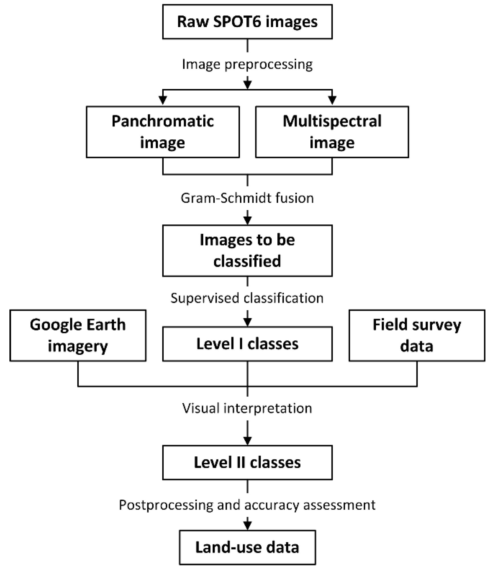
Figure 3.
Watershed division based on the fusion of the terrestrial features and digital elevation model.
Figure 3.
Watershed division based on the fusion of the terrestrial features and digital elevation model.
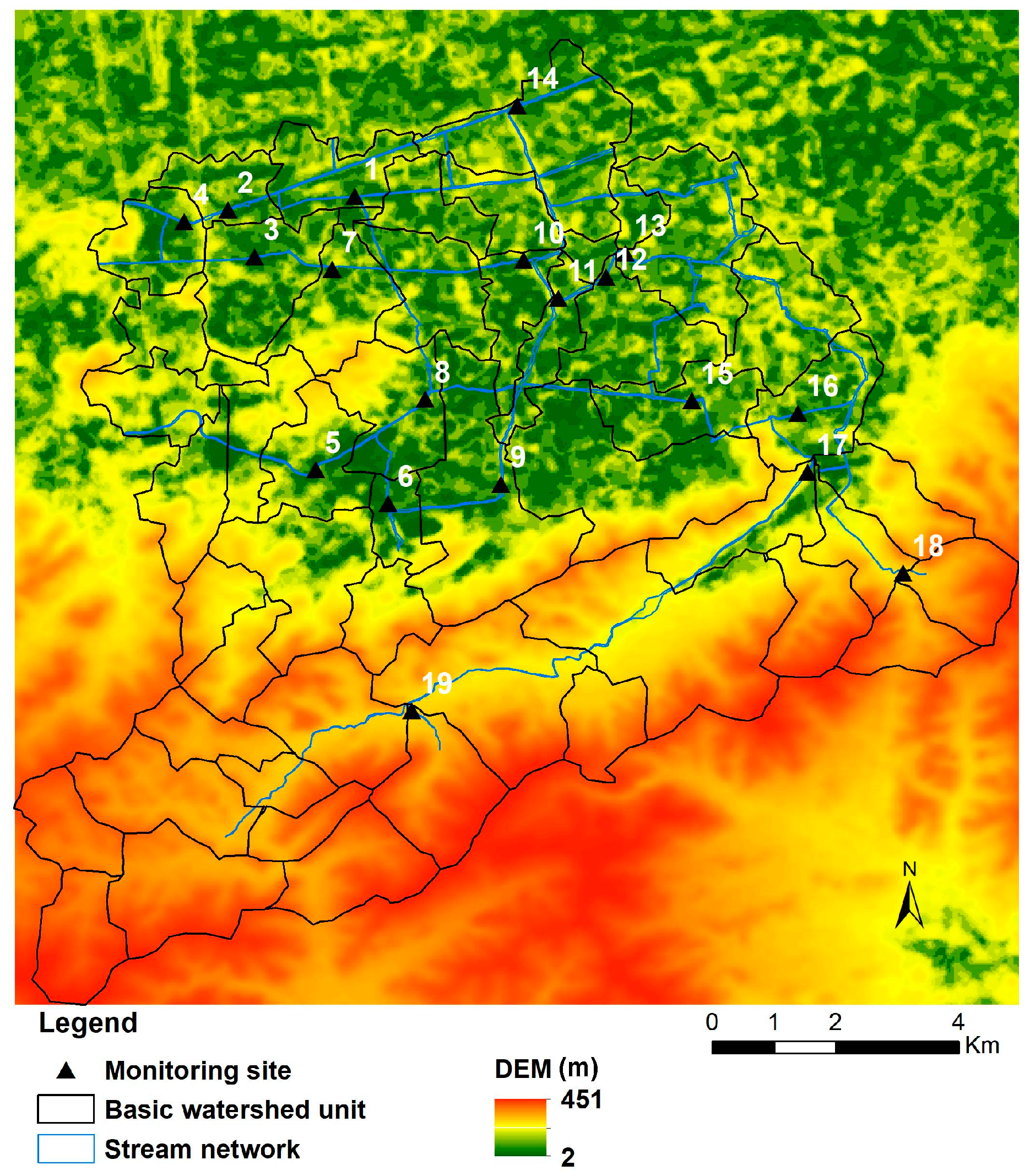
Figure 4.
Proportional area of each land use area at the catchment scale. The labels in the x axis indicate different catchments. The initial character “C” represents catchment, and the numerical values correspond to sampling sites.
Figure 4.
Proportional area of each land use area at the catchment scale. The labels in the x axis indicate different catchments. The initial character “C” represents catchment, and the numerical values correspond to sampling sites.
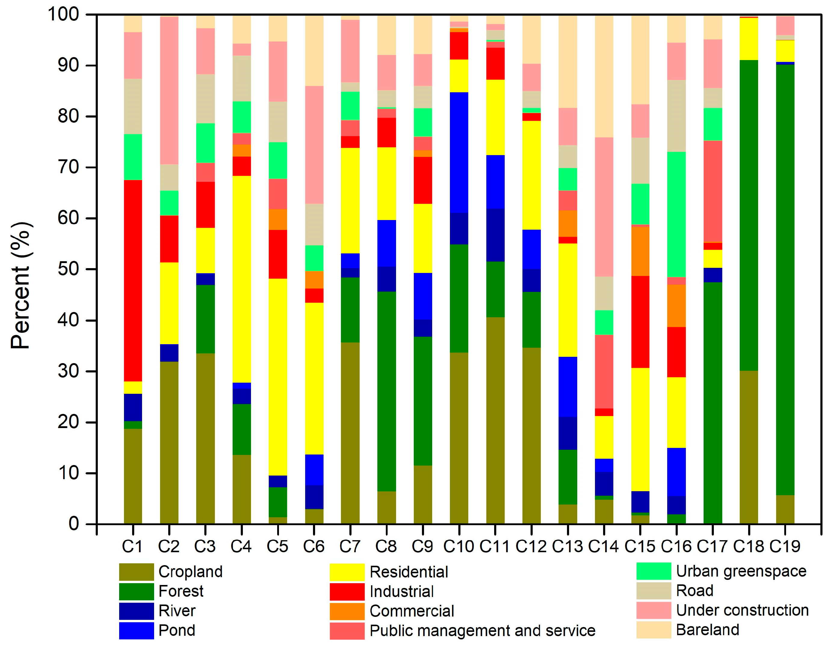
Figure 5.
Spatial variations of (a) TN, (b) TP, (c) TChla, (d) ChlaCyan, (e) ChlaChlo, and (f) ChlaBaci-Dino. The concentrations were classified into six classes based on the natural breaks method.
Figure 5.
Spatial variations of (a) TN, (b) TP, (c) TChla, (d) ChlaCyan, (e) ChlaChlo, and (f) ChlaBaci-Dino. The concentrations were classified into six classes based on the natural breaks method.
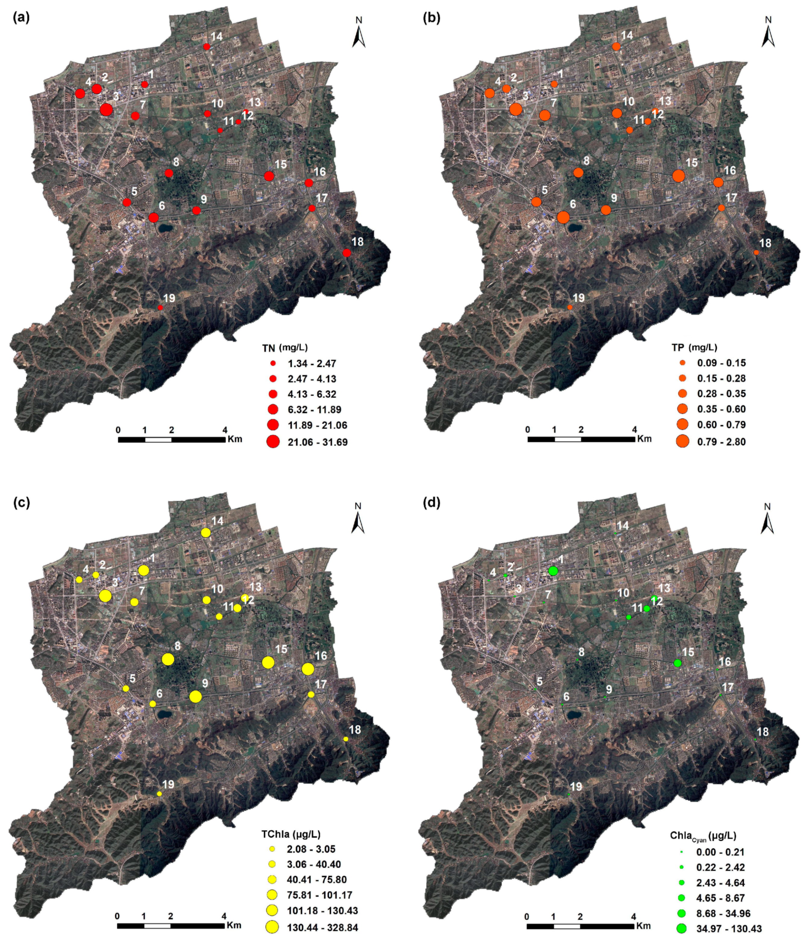

Figure 6.
Correlation coefficients between land use areas and water quality parameters based on Spearman’s rank order correlation analysis. One asterisk indicates p-value < 0.05 and two asterisks p-value < 0.01.
Figure 6.
Correlation coefficients between land use areas and water quality parameters based on Spearman’s rank order correlation analysis. One asterisk indicates p-value < 0.05 and two asterisks p-value < 0.01.

Figure 7.
Spearman rank correlation between water quality parameters and landscape metrics. One asterisk indicates p-value < 0.05 and two asterisks p-value < 0.01.
Figure 7.
Spearman rank correlation between water quality parameters and landscape metrics. One asterisk indicates p-value < 0.05 and two asterisks p-value < 0.01.
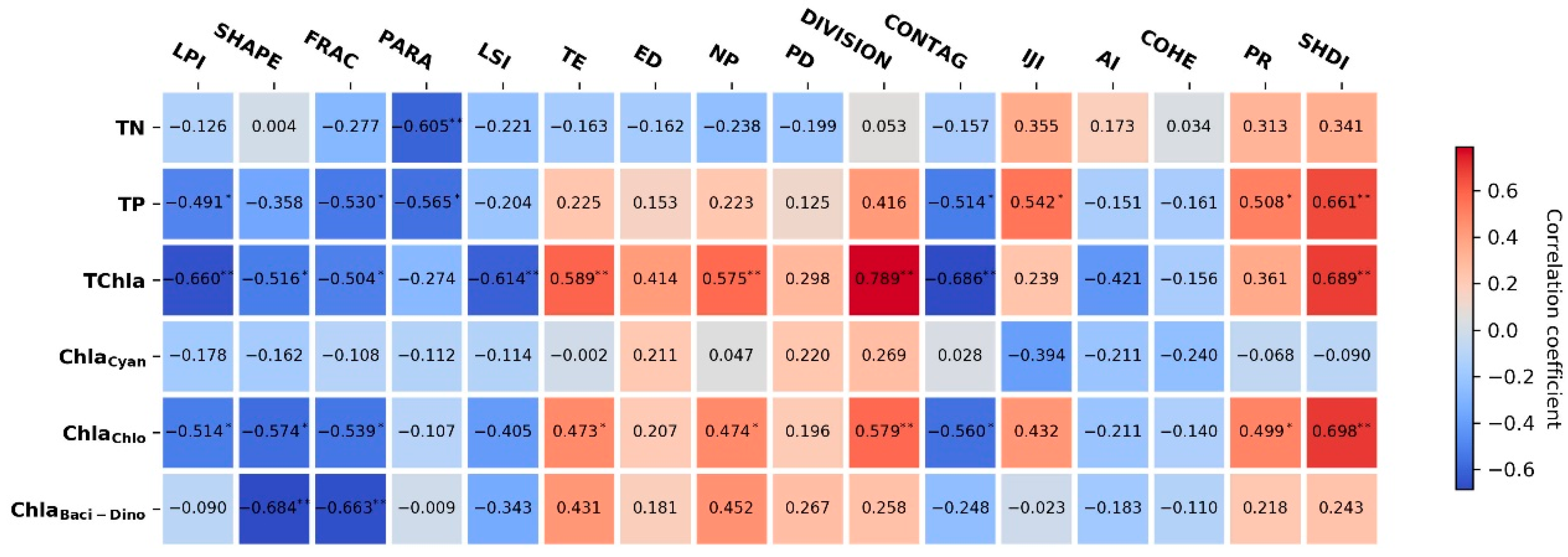
Figure 8.
Biplots of RDA about the water quality parameters (represented by dark blue lines) and landscape pattern metrics at land use class levels (represented by red lines), i.e., cropland (a), forest and water (b), built-up (c), bareland (d), and all land use types (e). The angle between the two arrows indicates the magnitude of the correlation. The angle less than 90° means positive correlation, the less the angle, the larger the correlation, and vice versa. The arrow length indicates to what extent the variance could be explained by the specific factor.

Table 1.
Abbreviations and descriptions of the selected landscape metrics.
| Category | Name (Abbreviation) | Unit | Description | Level |
|---|---|---|---|---|
| Dominance | Percentage of Landscape (PLAND) | % | Percentage of landscape comprised of corresponding patch type. | Class |
| Largest Patch Index (LPI) | % | The proportion of total area occupied by the largest patch of a patch type. | Class, Landscape | |
| Shape complexity | Mean Shape Index (SHAPE) | unitless | Mean patch perimeter divided by the minimum perimeter of the corresponding land use area. | Class, Landscape |
| Mean Fractal Dimension Index (FRAC) | unitless | The sum of 2 times the logarithm of patch perimeter divided by the logarithm of the total area for the corresponding patch type divided by the number of patches. | Class, Landscape | |
| Mean Perimeter-Area Ratio (PARA) | unitless | Equals 2 divided by the slope of the regression line obtained by regressing the logarithm of patch area against the logarithm of patch perimeter. | Class, Landscape | |
| Landscape Shape Index (LSI) | unitless | The perimeter-to-area ratio for the corresponding class. LSI increases with irregular shapes. | Class, Landscape | |
| Fragmentation | Total Edge (TE) | m | Equals the sum of the lengths of all edge segments involving the corresponding patch type. | Class, Landscape |
| Edge Density (ED) | m/ha | Total length of all edge segments divided by total area for the corresponding patch type. | Class, Landscape | |
| Number of Patches (NP) | unitless | Equals the number of patches in the landscape. | Class, Landscape | |
| Patch Density (PD) | n/km2 | Expresses the number of patches of the corresponding patch type per unit area. | Class, Landscape | |
| Landscape Division Index (DIVISION) | % | Equals to 1 minus the area of the plaque divided by the sum of squares of the landscape comprised of the corresponding patch type. | Class, Landscape | |
| Aggregation and Connectedness | Contagion (CONTAG) | % | Extent to which patch types are aggregated or clumped as a percentage of the maximum possible. | Landscape |
| Interspersion and Juxtaposition Index (IJI) | % | Equals the observed interspersion over the maximum possible interspersion for the given number of patch types | Class, Landscape | |
| Aggregation Index (AI) | % | Number of like adjacencies involving the corresponding class, divided by the maximum possible number of like adjacencies involving the corresponding land use type. | Class, Landscape | |
| Cohesion Index (COHE) | unitless | Indicates the physical connectedness of the corresponding patch type. | Class, Landscape | |
| Mean Contiguity Index (CONTIG) | unitless | Assessing patch shape based on the spatial connectedness of cells within a patch. | Class | |
| Diversity | Patch Richness (PR) | unitless | Equals the number of different patch types present within the landscape boundary. | Landscape |
| Shannon’s Diversity Index (SHDI) | unitless | Equals minus the sum, across all patch types, of the proportional abundance of each patch type multiplied by that proportion. | Landscape |
Table 2.
Statistics of stream water quality parameters.
| Indicator | Maximum | Minimum | Mean (std.) |
|---|---|---|---|
| TN (mg/L) | 31.69 | 1.88 | 6.54 (6.65) |
| TP (mg/L) | 2.80 | 0.09 | 0.62 (0.64) |
| TChla 1 (μg/L) | 328.84 | 2.08 | 102.49 (94.08) |
| ChlaCyan 2 (μg/L) | 130.43 | 0.00 | 9.9 (30.30) |
| ChlaChlo 3 (μg/L) | 233.29 | 0.00 | 68.44 (77.87) |
| ChlaBaci-Dino 4 (μg/L) | 138.74 | 0.00 | 24.15 (33.93) |
1 TChla: Total chlorophyll a concentration; 2 ChlaCyan: chlorophyll a concentration of Cyanophyta; 3 ChlaChlo: chlorophyll a concentration of Chlorophyta; 4 ChlaBaci-Dino: chlorophyll a concentration of Bacillariophyta and Dinophyta.
Table 3.
Spearman rank correlations between stream water quality parameters.
| TN | TP | TChla | ChlaCyan | ChlaChlo | ChlaBaci-Dino | |
|---|---|---|---|---|---|---|
| TN | 1 | |||||
| TP | 0.791 ** | 1 | ||||
| TChla | 0.269 | 0.677 ** | 1 | |||
| ChlaCyan | −0.429 | −0.327 | 0.067 | 1 | ||
| ChlaChlo | 0.541 * | 0.798 ** | 0.765 ** | −0.313 | 1 | |
| ChlaBaci-Dino | −0.167 | 0.097 | 0.35 | 0.121 | 0.318 | 1 |
* Correlation is significant at the 0.05 level; ** Correlation is significant at the 0.01 level.
Table 4.
Regression of water quality parameters against land use area.
| Response | Regression | Adjusted R2 | P |
|---|---|---|---|
| TP | TP = 0.215 + 0.127 × Industrial | 0.352 | 0.048 |
| TChla | TChla = 1.630 + 0.822 × Industrial + 0.656 × Bareland | 0.688 | 0.000 |
| ChlaChlo | ChlaChlo = 2.164 + 0.775 × Bareland | 0.437 | 0.035 |
| ChlaBaci-Dino | ChlaBaci-Dino = 1.025 + 0.761 × Bareland | 0.414 | 0.046 |
Notes: Only significant models (p < 0.05) are listed; The adjusted R2 (adjusted coefficient of multiple determination) was used to measure the predictive power of the model.
Table 5.
Regressions of water quality parameters against landscape metrics.
| Response | Regression | Adjusted R2 | P |
|---|---|---|---|
| TN | TN = 7.318 − 0.738 × PARA 1 | 0.463 | 0.025 |
| TP | TP = 3.108 − 0.359 × PARA | 0.396 | 0.033 |
| TChla | TChla = −2.342 + 6.297 × SHDI 2 | 0.722 | 0.000 |
| ChlaChlo | ChlaChlo = −2.766 + 6.080 × SHDI | 0.539 | 0.001 |
| ChlaBaci-Dino | ChlaBaci-Dino = 18.345 − 15.129 × SHAPE 3 | 0.455 | 0.004 |
Notes: Only significant models (p < 0.05) are listed; the adjusted R2 was used to measure the predictive power of the model. 1 PARA: Mean Perimeter–Area Ratio, 2 SHDI: Mean Shape Index, 3 SHAPE: Shannon’s Diversity Index.
Table 6.
Water quality variations explained by the landscape metrics in RDA.
| Land Use Class | Explained Variation (%) | Selected Explanatory Variables (p < 0.05) | ||
|---|---|---|---|---|
| Axis 1 | Axis 2 | All Axes | ||
| Cropland | 30.9 | 3.5 | 37.9 | 11SHAPE, 11FRAC |
| Forest and wetland | 40.8 | 10.9 | 54.6 | 21SHAPE, 31LSI, 32LSI, 31SHAPE, 31COHE |
| Built-up | 49.0 | 16.9 | 71.4 | 42CONTIG, 42COHE, 45PLAND, 45PD, 46PLAND, 46ED, 47PD |
| Bareland | 29.7 | 3.9 | 34.6 | 51PLAND, 51LSI, 51CONTIG, 51COHE |
| All types | 56.8 | 18.3 | 84.1 | 42COHE, 42CONTIG, 11FRAC, 11SHAPE, 51COHE, 31COHE, 31LSI, 51LSI, 32LSI |
Notes: The landscape metrics include the Edge Density (ED), Patch Density (PD), Percentage of Landscape (PLAND), Mean Shape Index (SHAPE), Mean Fractal Dimension Index (FRAC), Landscape Shape Index (LSI), Contiguity Index (CONTIG), and Cohesion Index (COHE). The numerical values in the “selected explanatory variables” column represent specific land uses, i.e., 11 (cropland), 21 (forest), 31 (river), 32 (pond), 42 (industrial), 45 (urban greenspace), 46 (road), 47 (under construction), and 51 (bareland). The p values were derived from Monte Carlo permutation tests (499 permutations) of all the canonical axes.
© 2020 by the authors. Licensee MDPI, Basel, Switzerland. This article is an open access article distributed under the terms and conditions of the Creative Commons Attribution (CC BY) license (http://creativecommons.org/licenses/by/4.0/).
Share and Cite
MDPI and ACS Style
Song, Y.; Song, X.; Shao, G. Response of Water Quality to Landscape Patterns in an Urbanized Watershed in Hangzhou, China. Sustainability 2020, 12, 5500. https://doi.org/10.3390/su12145500
AMA Style
Song Y, Song X, Shao G. Response of Water Quality to Landscape Patterns in an Urbanized Watershed in Hangzhou, China. Sustainability. 2020; 12(14):5500. https://doi.org/10.3390/su12145500
Chicago/Turabian StyleSong, Yu, Xiaodong Song, and Guofan Shao. 2020. "Response of Water Quality to Landscape Patterns in an Urbanized Watershed in Hangzhou, China" Sustainability 12, no. 14: 5500. https://doi.org/10.3390/su12145500
Note that from the first issue of 2016, this journal uses article numbers instead of page numbers. See further details here.