Conceptual Scheme Decision Model for Mechatronic Products Driven by Risk of Function Failure Propagation
by
 ,
,
Liting Jing
1,2, 
Qingqing Xu
1,
Tao Sun
1,
Xiang Peng
1,
Jiquan Li
1,
Fei Gao
2 and
Shaofei Jiang
1,* 1
College of Mechanical Engineering, Zhejiang University of Technology, Hangzhou 310023, China
2
College of Computer Science & Technology, Zhejiang University of Technology, Hangzhou 310023, China
*
Author to whom correspondence should be addressed.
Sustainability 2020, 12(17), 7134; https://doi.org/10.3390/su12177134
Submission received: 21 July 2020
/
Revised: 27 August 2020
/
Accepted: 28 August 2020
/
Published: 1 September 2020
Abstract
:Reliability is a major performance index in the electromechanical product conceptual design decision process. As the function is the purpose of product design, the risk of scheme design is easy to be caused when there is a failure (i.e., function failure). However, existing reliability analysis models focus on the failure analysis of functions but ignore the quantitative risk assessment of conceptual schemes when function failures occur. In addition, design information with subjectivity and fuzziness is difficult to introduce the risk index into the early design stage for comprehensive decisions. To fill this gap, this paper proposes a conceptual scheme decision model for mechatronic products driven by the risk of function failure propagation. Firstly, the function structure model is used to construct the function fault propagation model, so as to obtain the influence degree of the subfunction failure. Secondly, the principle solution weight is calculated when the function failure is propagated, and the influence degree of the failure mode is integrated to obtain the severity of the failure mode on the product system. Thirdly, the risk value of failure mode is calculated by multiplying the severity and failure probability of failure mode, and the risk value of the scheme is obtained based on the influence relationship between failure modes. Finally, the VIKOR (Višekriterijumska Optimizacija i kompromisno Rešenje) method is used to make the optimal decision for the conceptual scheme, and then take the cutting speed regulating device scheme of shearer as an example to verify the effectiveness and feasibility of the proposed decision model.
1. Introduction
Conceptual design decision is a major part of new product development (NPD). It seeks the value of schemes by decision objectives, judges, and rank candidate schemes with the help of multi-objective decision models to obtain the optimal scheme. The current mainstream decision model uses numerical methods to consider multiple design factors (i.e., cost, quality, reliability, etc.) to achieve the optimal decision of the conceptual scheme (CS) [1,2,3]. With the rapid development of technology, the rapid change of users’ requirements urges enterprises to develop a new product with a shorter cycle and lower cost [4]. However, this involves uncertainty and design risks, especially for complex electromechanical products such as aviation equipment and coal mine machinery equipment, the reliability of CS should be considered. Nowadays, the research of reliability analysis mainly focuses on the modeling of design risk propagation models [5], and the analysis of structural system failure modes in detailed design [6], which leads to concept design failure risk not being considered effective, and effective reliability evaluation data cannot be provided in CS decision process.
Since Stone et al. [7] introduced failure modes and risks in the function analysis stage, reliability has been extensively studied in conceptual design, mainly including three aspects, namely functional reliability analysis, failure risk identification, and principle solution reliability evaluation. In functional reliability analysis, Kurtoglu et al. [8] performed failure reasoning on functional failures to avoid the problem of functional failure. To reduce the impact of failure propagation on the system, Short et al. [9] proposed a function failure design method that sacrificed non-critical subsystems to maintain core functions, which could help designers complete primary mission objectives despite failure events. Later, based on the functional dependency network analysis model [10], Guariniello et al. [11] used system operational dependency analysis (SODA) to consider the internal state of the design system and better accounted for stochasticity to improve the efficiency of functional failure analysis. Although the methods above are helpful to improve functional reliability and support decision-making [12] and propose two strategies of prevention and sacrifice to ensure the realization of system functions, the qualitative dependence between functions will cause state changes of different failure models, making it difficult to provide quantifiable risk data for the decision process of CSs.
In the failure risk identification, Xiao et al. [13] analyzed multiple failure modes in FMEA (failure mode and effects analysis), which can be provided to other designers to prevent the hidden dangers caused by the failure mode. Then, in order to improve the reliability of the redesign, Ma et al. [6] used FMEA to identify the failure causal relationship between components and proposed a fuzzy permanent function to measure the internal failure effect of the conceptual scheme to ensure customer satisfaction. However, traditional FMEA is affected by cognitive preferences. For this reason, Baykasoğlu et al. [14] integrated fuzzy cognitive maps and FMEA to reliably obtain risk priority indexes. In addition, Hamraz et al. [5] proposed a multidomain engineering change propagation model based on the function-behavior-structure (F-B-S) linkage model to reduce the uncertainty of design risk. The above risk identification models mainly focused on the overall failure mode risk calculation in the scheme and considered the failure mode dependency to reduce the risk of the product. However, most pertinent studies did not analyze the failure risk of the principle solution in each CS, which cannot guarantee the reliability of the selected scheme.
In the principle solution reliability evaluation, O’Halloran et al. [15] analyzed the functional components with high risk and improved them to ensure the scheme’s reliability. Ma et al. [16] used the multi-objective decision model in a morphological matrix to seek the appropriate principle solution and combined with the reliability index to determine the optimal scheme. Due to the abstract nature of the principle solution, Aydoğan et al. [17] combined with the Z-axiomatic design theory to obtain the decisionmaker’s risk attitude about the scheme, thereby eliminating unreliable principle solution to enhance the success for a better decision. Besides, as far as possible to ensure customer needs on the premise of reducing the risk of principle solutions, Ma et al. [18] introduced fuzzy QFD (quality function deployment) and failure risk analysis model to identify principle solutions to be improved to redesign complex products. Although the above-mentioned decision model considers the influence of reliability indicators on the value of the scheme, it cannot identify the principle solution of the failure to the scheme risk. This limitation motivates the study as well.
For this purpose, how to analyze the impact of function failure propagation on the risk of CSs and integrate the scheme risk data in the decision process is still one of the most significant works to ensure the robustness and reliability of the CS, several shortcomings are found and listed as follows:
- The issue of ignoring the risk identification of dangerous functions and principle solution in the function failure propagation analysis process deserves to be well explored.
- The failure risk analysis method relies on experts’ evaluation of the probability for each failure mode and ignores the comprehensive analysis of the scheme risk of failure mode interaction.
- The process of scheme risk assessment in case of function failure involves subjectivity, a fuzzy logic model is necessary to be adopted to reduce the uncertainty of decision results.
It can be seen from the above that the traditional reliability decision model of CS does not consider the process of function failure analysis and reasoning, and ignores the risk impact of the failure of principle solution on the overall scheme value. To this end, the decision model for the mechatronic product conceptual scheme based on the function failure propagation analysis is proposed. After that, a function failure propagation analysis model and multiple propagation modes are constructed. Next, the risk propagation path of the CS is analyzed though the mapping process of requirement-function-principle solution (RFP), and the CS with the lowest risk value is determined. The remaining of this paper is organized as follows. Section 2 outlines the related works. The conceptual scheme decision model-based function failure relay analysis framework is proposed in Section 3. A cut speed regulating device of shearer as a case study to verify the proposed approach is taken in Section 4, and the paper ends with a conclusion and future work in Section 5.
2. Related Works
2.1. Conceptual Design Decision
Conceptual design decision plays a key role in subsequent design activities, which will directly affect the performance, manufacturing process, and cost objective of the product. Due to its importance in NPD, the decision-making of CS has always been an attractive topic among researchers. To effectively compare the value of different schemes, many numerical decision methods have been developed to select the optimal design scheme, as shown in Figure 1.
As a typical MODM problem, many decision models are used to integrate the value information of candidate schemes under multiple objectives to complete the ranking. Ma et al. [16] integrated customer needs and risk analysis to build a multi-objective optimization model to seek the appropriate principle solution. Saaty [19] proposed ANP (network analysis process) to construct the judgment matrix and calculate the weight of the evaluation objective. Ma et al. [1] used TOPSIS (the technique for order of preference by similarity to ideal solution) to analyze the sustainability of the product to formulate the optimal end-of-life strategy. Tiwari et al. [20] used VIKOR based on rough set (Višekriterijumska Optimizacija i kompromisno Rešenje) to find the optimal design scheme between cost and benefit objectives under uncertainty. Lo et al. [21] used QFD (quality function deployment) to construct 3D morphology diagrams in product variant design, so as to quickly generate CSs. Jing et al. [22] used fuzzy DEMATEL (decision making trial and evaluation laboratory) to analyze the causality between different objectives in the decision process, and form the game strategy to achieve the optimal decision of the scheme. In addition, the evaluation information mainly depends on the subjective judgment by experts, which makes decision results affected by factors such as expert knowledge background and skills, leading to uncertainty in the decision environment. Thus, researchers introduce rough sets, interval number, and fuzzy numbers to capture the uncertainty from the subjective judgment of experts. Ayağ [23] integrated fuzzy numbers and AHP (analytic hierarchy process) to evaluate the conceptual scheme. Zhu et al. [4] proposed a hybrid decision approach of TOPSIS and AHP and integrated fuzzy rough numbers to process evaluation data under uncertainty. Pamučar et al. [24] proposed a novel DEMATEL-ANP model based on interval rough numbers, and a new multi-attribute technique was applied to evaluate the design scheme.
Of course, as design data becomes more abundant and decision problems become more complicated, some decision algorithms are used for intelligent decision of products. For instance, Ferreira and Paulo [25] used the prediction ability of artificial neural networks to analyze multi-parameter problems, which could improve the quality of the decision result; Kang and Tang [3] used ant colony optimization model to automatically generate feasible schemes based on design structure matrix; Sibois et al. [26] used reliability-based stochastic Petri Net approach to realize the verification of engineering system to drive innovation concept design. The product conceptual scheme decision applications are also summarized as a picture at the end of this section.
In summary, most of the methods above mainly consider how to analyze the “value” differences between candidate schemes, and integrate evaluation data to achieve the optimal decision. However, existing research focuses on product design risk prediction [27] or function failure risk [28] but ignores the impact of the PRF of the risk path on scheme reliability in the conceptual design process, which also promotes the research in this paper.

2.2. Conceptual Design Failure Risk Analysis
Reliability analysis approach in NPD mainly include PRA (probabilistic risk assessment) [30], RBD (reliability block diagram) [31], FTA (fault tree analysis) [32] and FMEA [13]. Since the FMEA is a qualitative analysis and evaluation method that analyzes the potential failure modes of each component unit of the product to avoid high-risk failure modes, which has been widely used in the conceptual design process. Peeters et al. [33] integrated FTA and FMEA in a recursive manner, which is used to evaluate critical system-level failure modes to ensure product system operation. To reduce the uncertainty of risk assessment, Gu et al. [34] proposed an improved method of TOPSIS-based failure mode sequencing and solved the ambiguity of risk calculation. Chen et al. [35] combined with QFD and FMEA to develop a fuzzy linear programming model. In order to improve the accuracy of failure analysis, Xiao et al. [13] proposed a weighted risk priority number to calculate the risk value of multiple failure modes in FMEA. Ma et al. [29] used a directed failure causality network to quantify the failure risk of each component and selected the scheme with lower risk. Zammori et al. [36] identified the interaction between failure modes to calculate the risk priority number, which can solve the correlation problem in the CS evaluation process.
Function is the essence of conceptual design, and connecting design requirements and principle solutions. Reliability research on the product function can identify risks more efficiently [18]. Stone et al. [7] proposed a function failure design method, and constructed a morphological matrix of function-failure modes, using historical failure data to identify functions with a higher risk of failure; Huang et al. [37] used load-strength theory for reliability design at the conceptual design stage. Subsequently, to better assess of the risk of the CS when the function fails, Chen et al. [38] analyzed the failure risk based on the functional failure dependency and realized the quantitative risk assessment of the function failure; Yontay and Pan [39] used Bayesian network model to calculate the conditional probability between function and component failure and focused on the core function for risk analysis.
For function failures and propagation problems, Krus and Grantham [40] analyzed the propagation of failures through function failure chains to improve design defects; Kurtoglu et al. [41] proposed an FFIP (function failure propagation mode) to analyze the three elements of functional modeling, behavior simulation and failure reasoning; Wang et al. [42] proposed a failure propagation path search approach for electromechanical systems; Mehrpouyan et al. [43] introduced an MFIP (model-based failure identification and propagation) framework in avionics systems to identify security issues caused by environmental disturbances and subsystem failures.
The published literature can effectively solve the failure propagation model of the product system, and propose the evaluation model to judge the system risk. However, how to apply the function failure propagation model to the calculation of the system impact degree when the function failure occurs, and quantify the risk value of the principle solution in the RFP mapping process under uncertainty, which all have not been considered in the existing literature.
3. Proposed Method
Figure 2 shows the decision framework of the mechatronic product conceptual scheme based on functional failure propagation analysis, which is mainly divided into five parts. The specific solution steps are as follows.
Step A1: Sub-requirement-subfunction correlation matrix and subfunction autocorrelation matrix are constructed, and the sub-requirement weight () is transformed into the function importance ().
Step A2: The propagation path of function failure is analyzed, and the function structure model is transformed into a directed weighted functional network model. Then, the influence (LR) of subfunction nodes in the directed graph is calculated by using the LeaderRank algorithm [44]. Next, the importance () of function is transformed into the weight () of principle solution through the house of quality (HOQ) [32] and fuzzy number [23].
Step A3: Bayesian network model is used to analyze the importance (I) of multiple failure modes to the principle solution (i.e., the influence of failure modes on the principle solution). Then, the severity () of the failure mode is calculated by combining the weight () and the importance (I) on the principle solution.
Step A4: The failure rate () of each failure mode is obtained from the database, and the risk value () of failure mode is calculated by integrating the rate () and the severity of failure mode ().
Step A5: By analyzing the interaction between failure modes, influence the relationship matrix of the failure mode is constructed to calculate the principle solution risk value () and the risk value () of the overall scheme, and then the optimal CS is decided by the VIKOR method [45].
3.1. Function Failure Propagation Model
The purpose of product conceptual design is to obtain the CS with one or more functions, and, under the RFP mapping relationship, failure analysis around function solving process can effectively identify potential faults. Thus, by constructing a failure propagation model to analyze the propagation path of the function failure in the system, and to evaluate the impact of the failure on the product system, which is an important part of the risk assessment of the CS. Based on the relationship between the subfunction and the function flow in the function structure model, the propagation modes of function failures are divided into 3 types with respect to failure propagation path, as shown in Table 1.
The definition of the function failure propagation mode is as follows:
- Propagation mode I: the failure propagation path propagates in a direction parallel to the function flow;
- Propagation mode II: the failure propagation path propagates the failure in the opposite direction to the function flow;
- Propagation mode III: the failure propagation path indirectly propagates failures along two or more continuous function flow.
According to the propagation mode of functional failure, the propagation of failure will change the influence of function on the system, so it is necessary to analyze the failure propagation path to obtain the influence degree (ηj) of function failure. For this purpose, this paper constructs a directed functional network diagram (DFND) [29] to convert the functional structure model to DFND and analyzes the failure propagation type of a certain subfunction. Next, based on the DFND, the impact of the fault is analyzed, thereby reducing the design Risk, as shown in Figure 3.
DFND can be described as DF = (K, L, FL), where K represents the set of all nodes, the nodes correspond to the subfunctions in the function structure model, and K = (k1, k2, …, kα), G = {1, 2, …, α} L represents a set of directed edges, and the directed edges correspond to the path of function failure propagation, are shown in Equation (1). FL represents the set of flows on the directed edge so that the DFND is converted into an adjacency matrix FL with α×α elements, as shown in Equations (2) and (3).
3.2. Calculation of Principle Solution Weight Based on Function Failure Propagation Model
3.2.1. Analysis of the Propagation Model
In the process of function failure propagation analysis, the direct impact of functional failure (i.e., propagation mode I) needs to be considered first, which has the highest frequency and is the main way in failure propagation. When the failure of a subfunction is judged to have a direct impact, the corresponding subfunction flow in the function structure model is transformed into the directed edge in the directed weighted network diagram. Based on the transfer of subfunction flow in the function structure model, the flow of DFND directed edge is obtained. In this paper, the flow of subfunction flow is set as “1” and “2”, which respectively indicate that they are important and very important to the normal operation of the system [46], and the specific flow value is determined by the design experts.
For instance, the function structure of the thin-film solar cell example described in Figure 4 is divided input power (SF1), separate mixture (SF2), conduct vacuum (SF3), convert electrical energy into thermal energy (SF4), and heat mixture (SF5), and pilot air (SF6). It can be seen that the subfunction SF5 depends on the three function streams of SF2, SF3, and SF4, and the subfunction SF6 depends on the function stream of SF5. When the subfunction SF3 fails (i.e., the conduction of CdTe fails), or SF4 fails (i.e., cannot be converted to heat), both will cause the sub-function SF5 to fail. In addition, the failure of SF5 will directly affect SF6.
In the DFNF of Figure 5, when the SF2 fails (i.e., cannot realize the separation), the SF5 will fail. Therefore, a directed weighted network is determined along the direction of the function chain in the directed weighted network diagram. Then, the flow rate of the directed edge can be obtained by combining these two functional flows, as shown in Equation (4).
where flk(a,b) represents the flow of k-th associated functional flows to be merged, and σk represents the importance of the functional flows.
Further analysis of failure back-propagation (i.e., propagation mode II), back-propagation is that the failure of the latter subfunction reversely affects the previous subfunction. When it is judged that the failure of a certain subfunction will be back-propagated, a directed edge opposite to the direction of function flow is added in the directed weighted network diagram.
Finally, the indirect effect of function failure (i.e., propagation mode III) is considered. In this propagation mode, for example, when the failure mode of subfunction (SF4) is that the output heat energy is suddenly high or low, it will be transferred along SF5 to SF6, causing the failure of SF6. Thus, a directed edge from SF4 to SF6 is shown in Figure 5.
3.2.2. Influence Degree of Function Node in DFND
By analyzing the propagation path of functional failures, it is necessary to obtain the degree of impact of function failures on the product system. In the DFND, failure propagation can be regarded as a random propagation process. There is a mutual coupling between subfunction nodes. The random propagation events of each node will change the influence of the surrounding node failure, which is easy to form large calculation data. In this paper, the LeaderRank algorithm of web page ranking [44] is used to calculate the influence of function failure after a random walk. Thus, the Leaderank algorithm in DFND can be used to ensure the realization of core subfunctions to reduce the risk of design. The calculation steps of LRj of the sub-function node are as follows:
Step B1: The probability of node ka random walk towards node kb is pk(a,b), and its relationship with the flow into node kb is shown in Equation (5). Through random walk events, a transformation matrix PK is obtained, as shown in Equation (6).
where fl(a,b) represents the flow value between node ka and node kb.
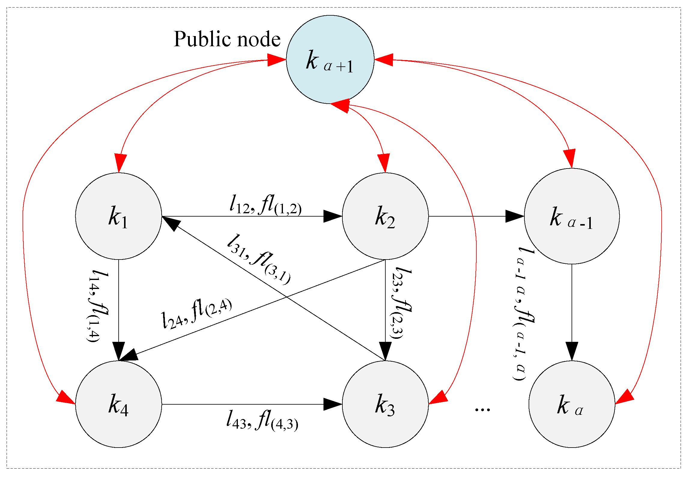
Step B2: By adding a public node on the basis of the original DFND and constructing the edge between the public node and other nodes, as shown in Figure 6. Then, the adjacency matrix FL’ is constructed by adding a node in the matrix FL, as shown in Equations (7) and (8).
Step B3: Since a public node is added, and this node in DFND is related to other nodes, the adjacency matrix in the random walk process changes, and the matrix PK’ is obtained, as shown in Equations (9) and (10).
Step B4: Initialize the influence value of function node j (1 ≤ j ≤ J) and public node, as shown in Equation (11).
Step B5: After t iterations, the matrix PK′ will remain stable, and the LRj(k) of the function node kj is equal to the value of all other function nodes flowing into this node after being evenly divided. The iteration formula is shown in Equation (12).
where fl(j′,j) is the flow from node kj′ to node kj in the matrix, and is the out-degree of node kj′.
Step B6: When the algorithm converges, the value of the public node is evenly distributed to the subfunction nodes, and the final value of each node is the LeaderRank value (LRj), as shown in Equation (13). LRj represents the influence degree of the function node, and the larger the value, the more influential it is in the propagation model.
where LRj(tc) is the value of the node kj in the steady-state, LRα + 1(tc) is the value of the public node in the steady-state, and α is the number of nodes in the DFND excluding the public node.
3.2.3. Calculation of Influence Degree of Function Failure
Product design requirements are composed of multiple sub-requirements i with various weights (rwi, 1 ≤ i ≤ I), which will directly affect subfunctions and indirectly affect other subfunctions [47]. To this end, the correlation between sub-requirements and subfunctions is expressed by constructing the sub-requirement–subfunction matrix. Therefore, the weight of the customer requirement (rwi) can be effectively transformed into the importance (fwj) of the subfunction.
However, the relationship between requirements is fuzzy and it is difficult to judge accurately. To this end, linguistic terms {very strong (VS), strong (S), medium (M), weak (W), and very weak (VW)} are used to express the relationship. Then the linguistic terms can be transformed into triangular fuzzy numbers (), where xl ≤ xm ≤ xu, and the triangular fuzzy numbers corresponding to the five linguistic terms are described in Table 2. The algebraic operation of the fuzzy value is shown in Equation (14).
The judgment matrix between sub-requirements is constructed by using the AHP method [19] and its eigenvalues are obtained. On the premise of meeting the consistency index CR, the weight value (i) of sub-requirement is calculated by Equation (15). Meanwhile, using the approach proposed by Ayağ [23], and by defining the interval of the confidence level β, the fuzzy number can be transformed into an interval value by Equation (16). Thus, the fuzzy weight i of the sub-requirement can be transformed into interval value i. Generally, to keep a moderate attitude, β is used to select 0.5 [48].
where xib represents the relative importance between sub-requirement i and b.
It can be seen that the greater the requirement’s weight is for the functions associated with requirements, the more serious the consequences of the failure of corresponding functions [15]. For this reason, it is necessary to clearly analyze the impact of functional failures on product systems. Then, the sub-requirement-subfunction correlation matrix and subfunction autocorrelation matrix is constructed through the RFP mapping process. Later, the fuzzy evaluation number transformed by Equation (16) is the interval value, as shown in Figure 7, where ij represents the interval correlation value between sub-requirement i and subfunction j, and ja represents the interval correlation value between the subfunction j and a.
Next, calculate the interval importance of subfunctions, as shown in Equation (17).
where j represents the interval importance of subfunction j, and i represents the interval weight of sub-requirement i.
Based on the function failure propagation model in Section 3.1, the propagation path of function failures is analyzed, and the influence degree LRj of each subfunction node is calculated by LeaderRank. At the same time, LRj is used to modify the importance of subfunctions by Equation (18) to obtain the interval influence degree (j) of function failure.
3.2.4. Calculation of Principle Solution Weight Based on Function Failure Influence Degree
The HOQ of the subfunction-principle solution is shown in Figure 8. The roof of the HOQ is used to express the correlation of the principle solution of the failure. The failure relationship of the principle solutions refers to the correlation strength on the physical structure between the principle solutions, that is, the interaction between the spatial position and the physical connection between the principle solutions. In Figure 8, ij describes the interval correlation value between the subfunction j and the principle solution k (1 ≤ k ≤ K), and k1k2 represents the interval correlation value between the principle solution k1 and k2 in case of a fault.
The interval weight k of the principle solution k is calculated by Equations (19) and (20).
3.3. Failure Mode Risk Analysis of Principle Scheme Based on Bayesian Network Model
3.3.1. Failure Mode Severity for Product System Analysis
The severity of the failure mode n (1 ≤ n ≤ N) represents the value that leads to a reduction in the safety of the entire system, loss of functions, and performance degradation when the failure mode occurs. To intuitively analyze the risk of CS when the failure occurs, it is necessary to consider the degree of the principle solution of the failure after the failure mode occurs (i.e., the importance of the failure mode (Ikn)). Then, combining the Ikn and the k, the severity (kn) of failure mode to the whole system can be calculated.
To describe the multiple states of the failure mode, the set {no failure, minor failure, complete failure} is used to describe the three states of the failure mode, and the set {0, 0.5, 1} is used to represent the corresponding failure state. Then, based on the Bayesian network model, the influence of failure modes on the principle solution is analyzed. The root node is represented as the failure mode, and the leaf nodes are represented as the principle solution. Furthermore, the conditional probability table of each principle solution about different failure modes is obtained through expert survey data, as shown in Table 3. For instance, the failure modes x1, x2, x3 are the root nodes, and there are 9 (3^3) state combinations of the failure mode for three nodes.
The Ikn of failure mode (xn) refers to the average influence of all failure states for the failure mode (xn) on the principle solution failure state as T = Tq (i.e., the probability that all failure states of xn cause the principle solution failure state T = Tq). The importance calculation of the root node xn is shown in Equation (21).
After the importance, Ikn is calculated and multiplied by the weight k of the principle solution, the interval severity kn of the failure mode to the system is obtained, as shown in Equation (22). Next, normalize the severity based on Equation (23) to obtain the interval severity ′kn.
3.3.2. Calculation of the Risk Value of Each Failure Mode
Step C1: Obtain the failure probability of the principle solution. From the reliability database of non-electronic components NPRD-95 database [49], the failure rate of each principle solution has multiple data sources, and the maximum failure rate λkmax and the minimum failure rate λkmin are selected to obtain the failure rate of principle solution as shown in Equation (24).
Step C2: Obtain the failure probability of failure mode. From the failure mode distribution database of FMD-97 [44], the failure proportion of each failure mode for the principle solution is found. Then the failure rate ξkn of the failure mode is calculated by multiplying the Equation (25) with the principle solution of the interval failure rate k. Then, the relative failure rate ′kn is obtained by normalizing the failure rate based on Equation (26).
Step C3: Calculate the relative risk of failure modes. The two major influencing factors of failure mode risk are failure probability and failure severity [50]. The interval risk value kn of failure mode is calculated according to the probability ′kn and severity ′kn of failure, as shown in Equations (27)–(29).
3.3.3. Risk Value Assessment of Principle Scheme
In the actual operation process of the product, there are many reasons for the system failure, which are mutual influence between the failure modes. To consider this relationship, this research conducts risk assessment on the correlation between failure modes, and constructs a directed graph of failure mode influence relationship, as shown in Figure 9. The grey box represents the failure mode and its risk value, the directed edge can describe the influence relationship between the failure modes.
According to the above digraph, the influence relation table between failure modes is obtained, as shown in Table 4. In the table, kn represents the interval risk value when the failure mode occurs, and the weight Pζn on the directed edge indicates the influence intensity of failure mode Fkζ on Fkn. In addition, Pζn is quantified by a fuzzy number, and the weight is set as {0.1, 0.3, 0.5, 0.7, and 0.9}.
Through the relationship of the failure modes in Table 4, the influence relationship matrix V′ of the failure modes is characterized as:
In order to measure the overall risk situation after all failure modes interact in the principle solution, the risk value (k) integrated model of the principle solution is calculated by Equation (32).
The terms of all the sub-parts in Equation (32) is explained as follows:
- is the sum of risk values when all failure modes in the current principle solution (k) occur separately
- is the sum of risk values in case of double failure
- 1/3 is the sum of the risk values of triple failure
- 1/z is the sum of the risk values of z failures, and z is the number of elements in the set Z.
Based on the mapping relationship between principle solution and subfunction, the interval risk value of a conceptual scheme is calculated based on the interval risk value of principle solution k, as shown in Equation (33).
3.4. The Optimal Scheme Decision Based on VIKOR Model with Considering the Risk Value
Firstly, the risk value of the CS is taken as one of the evaluation objectives, and other evaluation objectives ξ (1 ≤ ξ ≤ T) are determined. Then, the experts make a fuzzy judgment on the CSr (1 ≤ r ≤ R) based on the objective ξ, and integrate the risk value of the CSr, so as to obtain the comprehensive value of the scheme, and the decision matrix M is shown in Equation (34).
where rξ is the evaluation data of conceptual scheme r in the objective ξ.
Later, the decision matrix is standardized by Equation (35). At the same time, with the help of Equation (16), rξ is transformed into the interval number rξ as shown in Equation (36).
Finally, the VIKOR model is introduced, which is it is a compromise solution close to the ideal solution [51], and realize the ranking of multiple concept schemes. The steps are as follows:
Step D1: The positive ideal parameter mξ+ and the negative parameter mξ- in the normalized decision matrix N are selected. For benefit objective, mξ+ = maxrmUrξ, mξ− = minrmLrξ; and for cost objective, mξ+ = minrmLrξ, mξ+ = maxrmUrξ.
where B is the benefit objective set, and C is the cost objective set.
Step D2: Calculate the maximum group benefit Sr and the maximum individual regret Rr, as shown in Equations (39) and (40).
where wξ is the weight of the evaluation objective ξ.
Step D3: Calculate the comprehensive index Qr.
where S+ = maxrSr, S− = minrSr, R+ = maxrRr, R− = minrRr, and we choose v as 0.5 to maximize the group benefits and minimize the individual regret.
Step D4: The speed regulation schemes are sorted based on Qr, and the rank results are verified by Equation (42), so as to select the scheme with the best comprehensive benefits and the least risk.
where and represent the comprehensive index of the first and second schemes respectively.
4. Case Study
The shearer is the most important mechanical equipment in coal mining work [52], and the cutting part is one of its main mechanisms, as shown in Figure 10. The cutting device in the shearer mainly undertakes the function of coal cutting, and by adjusting the height of the rocker arm (blue mark in the figure), the continuous cutting and loading of cutting drum can be realized. The power is output to the cutting roller of the shearer through the transmission device, and then the core subfunction “cutting coal” is realized. Nowadays, in order to satisfy the cutting requirements of different coal qualities, it is necessary to improve the design of the shearer cutting device to achieve the above design requirements.
4.1. Function Failure Propagation Model of Cutting Speed Regulating Device
Through the analysis of the total demand of shearer “cutting speed change”, the following two cutting speed regulating devices are obtained: CS1: motor—spur gear—frequency conversion motor—gear pair—speed control turntable—variable speed gear pair—planetary gear train—roller; CS2: Motor—spur gear pair—hydraulic pump—relief valve—directional valve—hydraulic motor—differential gear train—planetary gear train—roller, and are shown in Figure 11.
The CS1 is a cutting speed adjustment device based on a variable speed gear pair. Firstly, the gears are driven by the motor to rotate, and different gears are engaged by the speed control turntable. Secondly, the frequency of the frequency conversion motor is changed to obtain different gear speeds. Thirdly, the planetary gears are used to reduce the speed and increase the torque. Finally, complete the coal cutting work through the rollers.
The CS2 is a cutting speed adjustment device that changes the speed through a hydraulic drive differential gear train. Firstly, the gears are driven by the motor to rotate. Secondly, the hydraulic output pressure is driven by the hydraulic motor to complete the movement of different transmission gears; thirdly, the different speeds are switched based on the differential gear train. Finally, the planetary gear train is used to output torque and speed, so that the rollers could complete the coal cutting work.
Then, based on the system design method [47], the subfunction set of cutting speed regulating device is abstracted, and the function structure model is constructed. Subsequently, according to the relationship between subfunction in the function structure model, the propagation mode of function failure is obtained. Due to the length limitation of the article, this section takes CS2 as a case study to conduct function failure propagation analysis and risk value calculation, as described in Figure 12.
4.2. Principle Solution Weight Calculation Based on Function Failure Propagation Model
(1) Sub-requirement weight analysis. After confirming with several users, the design sub-requirements are as follows: output multiple speed (SR1), low cost (SR2), not prone to failure (SR3), and stable power output (SR4). Through pairwise comparison of sub-requirements, the judgment matrix of cutting speed regulating device is constructed, as shown in Table 5.
After replacing linguistic terms with triangular fuzzy numbers in Table 2, the fuzzy numbers are converted into interval values by using Equation (16). The maximum eigenvector λmax = 0.9 and eigenvalue n = 6.5 are calculated by AHP model. At this time, the judgment consistency index CR ≤ 0.1, which proves that the judgment matrix has satisfactory consistency. Then, the weights (i) of sub-requirements are calculated by Equations (15) and (16), which are [0.28, 0.34], [0.13, 0.16], [0.23, 0.29], [0.17, 0.21].
(2) The function importance is calculated. In Figure 9, the subfunctions related to SR1 include SF3, SF5, SF5, SF8, and SF9. The sub-requirement-subfunction correlation matrix and subfunction autocorrelation matrix of CS2 are obtained by experts’ evaluation, as shown in Table 6 and Table 7.
By transforming the linguistic terms in the two correlation matrices into TFN, and calculating the importance (j) of subfunctions related to SR1 in CS2 based on Equation (17), as shown in Table 8.
(3) The influence degree analysis of function failure. Based on the function failure propagation model, the subfunctions are transformed into nodes in DFND, the propagation path of function failure is analyzed. Next, the function structure model is transformed into a directed weighted functional network diagram, as shown in Figure 13.
In Figure 13, a public node of subfunction is added to construct the adjacency matrix, and the influence degree LRj of each subfunction node is calculated by using the LeaderRank algorithm (Equations (5)–(13)). Therefore, the importance of subfunction is adjusted by using Equation (18), and the influence degree ηj of subfunction nodes SF3, SF5, SF7, SF8 and SF9 in the two CSs is calculated, as shown in Table 9.
(4) The principle solution weight recalculation. Construct the HOQ between the subfunctions of CS2 and the principle solution, as shown in Figure 14. Among them, the grid in the middle of the HOQ indicates that there is no mapping relationship between the subfunctions and the principle solution, while the lattice on the roof indicates that there is no mapping relationship between subfunctions.
By transforming the linguistic terms in the HOQ into TFN, the correlation between the subfunction-principle solution is obtained, and the weight k of the principle solution is calculated based on Equations (19) and (20), as shown in Table 10.
4.3. Calculation of Cutting Speed Regulation Scheme Risk Value of Failure Mode
Step E1: Acquisition of the failure mode of the principle solution. The failure state of shearer in operation is uncertain, and the principle solution of the failure mode is diverse. In the process of failure evolution, in addition to no failure state and complete failure state, there are also slight failure states. Based on the Bayesian network model, the influence of failure mode on principle solution is analyzed. The principle solution and corresponding failure mode of leaf node are shown in Table 11. Then, the importance of the principle solution of the “overflow valve” failure mode is illustrated as an example, and the risk value of the principle solution is calculated.
Step E2: Calculation of the risk value for the failure mode. The conditional probability table of the principle solution is obtained by analyzing the failure performance of the “overflow valve” in similar products and expert experience, as shown in Table 12.
From the above table, the failure mode “valve core stuck” is root node x221, failure mode “internal leakage” is root node x222, and the failure condition of the overflow valve is leaf node T22. Then, the risk value of failure mode is obtained based on the Equations (27)–(29), and the results are shown in Table 13.
Step E3: Calculation of the risk value of the CS. Taking the principle solution of the “hydraulic pump” as an example, the risk value of the hydraulic pump is calculated by using the risk assessment model of the principle solution in Section 3.3.3. The hydraulic pump has four failure modes: “internal leakage”, “suction”, “contaminated oil” and “damaged seal”. Based on the influence relationship between failure modes, the causality diagram of failure modes in the hydraulic pump is constructed, as shown in Figure 15, and the influence relationship between failure modes as shown in Table 14 is formed.
After obtaining the risk value kn and the influence relationship of failure mode, the interval risk value of each principle solution can be calculated by using a risk value integrated model. Taking the principle solution of the hydraulic pump as an example, the risk value R1 of the hydraulic pump is calculated by Equations (30) and (31), as shown in Equation (43).
Similarly, the risk value of each principle solution can be obtained, and the VaR of the overall scheme can be calculated, as shown in Table 15.
4.4. Optimal Decision of Cutting Speed Regulating Device Based on VIKOR
Through Step E1–Step E3, the risk value of the above two CSs can be obtained, and the speed control performance objective (PO) and economic objective (CO) can be set. For the objective CO, three experts judge it by fuzzy number, and obtain the average value of multiple TFNs. For the objective PO, the physical model-based graphical modeling software AMESim [53] is used to realize the preliminary simulation of the CS. AMESim software can effectively analyze the performance value of early design schemes without the modeling advantage of detailed structural parameters, as shown in Figure 16.
After that, the relationship between the roller speed and time for the CS simulation model is analyzed, then the time taken from the fluctuation state of the drum speed to the steady-state is obtained and used as the evaluation value of the speed control performance, as shown in Figure 17.
Finally, the risk value and the evaluation data of the scheme under PO and CO are integrated, and the data is preprocessed using Equations (34)–(36) to form a decision matrix N, as shown in Equation (44).
where F1, PO1, and CO1 respectively represent the risk value, performance value, and economic value of the CS1.
Determine the ideal value mξ+ and the negative value mξ- in the decision matrix N. Next, the comprehensive index Qr is calculated by Equation (41) and the optimal CS is selected, and the results are shown in Table 16.
It can be seen from Table 16 that the ranking result of the conceptual schemes is: CS2 > CS1, and the comprehensive design value of the scheme is consistent with the value of risk. Therefore, it can be seen that the risk value of the scheme plays a key role in product design, and the smaller the risk value, the stronger the robustness of the scheme in subsequent development.
5. Discussions
In the case study, the average risk values of the CS1 and CS2 are 0.526 and 0.464, respectively. It is proved that risk has a great influence on the comprehensive value of a design scheme in the VIKOR decision model. As stated in Section 4.3 above, although CS2 has one more principle solution than CS1, and the risk value of the hydraulic pump in CS2 is 0.210 greater than that of a motor in CS1 is 0.156, and the risk value of the reversing valve is increased (0.056, 0.110). The risk value is reduced on the whole (0.526 > 0.464), because the hydraulic motors and reversing valves that undertake the main functions have a low risk of failure. Then, it can be seen that the cutting speed regulating scheme driven by hydraulic pressure is more suitable for the coal mining environment, which can reduce the possibility of the risk of the scheme. Thus, the proposed risk value integration model of the principle solution can effectively adapt to the risk propagation environment of interactive failure mode. One potential avenue of future work is to analyze the influence of engineering system on external operation behaviors (e.g., human factors, environmental factors, etc.), so as to screen out the behaviors that are most sensitive to design risks and ensure the maximum decision value of the scheme. Further discussion of this can be found in Section 6.
Of course, the conceptual scheme decision model based on functional failure propagation can have a positive impact on the design of complex equipment systems. In these works, functional failure and risk increase will cause irreparable loss and damage in the subsequent product structural design, including the conceptual design process of hulls, weapon equipment, vehicle, etc. For example, the vehicle conceptual decision result with considering function failure propagation has stronger reliability, and the better the safety performance is. Then, the low-risk principle solution is selected on the basis of ensuring the function realization to provide effective principle solution strategy for vehicle robust design, and the key point is to avoid successive iterative optimization.
6. Conclusions and Future Work
With the increasing awareness of concept design decision reliability, the proposed decision method originally takes function failures into consideration in the risk quantitative calculation process of each principle solution and constructing a conceptual scheme decision model driven by the risk of function failure propagation. Firstly, the directed function network diagram (DFND) through function structure model is constructed; secondly and the LeaderRank algorithm is used to adjust the influence degree of functional failure; thirdly, the weight of each principle solution is analyzed in the function mapping process; fourthly, the influence of each failure modes on the principle solution is analyzed, which can obtain the severity of the failure mode on the product system. Finally, the risk of each CS is calculated based on the interaction of failure modes and the severity of principle solution, which is one of the important evaluation objectives to realize the optimal decision. The end decision result of the cutting speed regulating device scheme is to explain the influence of the scheme risk on the design value in more depth and understand the influence of different failure modes on the principle solution risk at the early design phase.
In this study, we calculate the risk value of principle solution in each CS and integrate it into the risk value of the scheme, which could solve the problem of difficulty and uncertainty in calculating the risk value. Compared with the previous failure propagation model which can only identify the propagation path, but cannot quantitatively analyze the risk numerical solution problem of the principle solution after the function failure propagation [26,27], we use the propagation process of multi-fault modes with different functions to intuitively calculate the specific principle solution risk value. More importantly, the fuzzy logic model is used to quantify the subjective information in the decision process, as well as the construction of the correlation matrix, which can reduce the uncertainty of decision results. Furthermore, a case study of a cutting speed regulating device scheme of shearer verifies the proposed approach can effectively solve the conceptual scheme decision problem with consideration of function risk propagation.
In summary, the contribution of this research is mainly shown in the following three parts: one is to realize the quantitative analysis of function failure propagation based on FMEA theory and RFP mapping process and provide risk assessment data for scheme decision. Second is to construct a risk value integrated model (Equation (32)) of the scheme by analyzing the interaction between the failure modes, which can comprehensively consider the overall risk of the scheme. Third is to numerically calculate the risk value of the principle solution after the failure propagation by constructing the multi-function failure propagation path in the conceptual design stage.
In the future, the development of the proposed method will involve the improvement of the analysis software for efficiency and usability. By constructing a graphical user interface to support new users to quickly understand and calculate the risk value of the conceptual scheme. In addition, human subjective behavior errors are considered to be the main reason for most failures in complex engineering design, which pose a greater challenge to the conceptual scheme decision. To this end, the following two aspects may be examined in future studies: (1) consider human factors and engineering factors to make the design scheme more harmonious; (2) establish a fuzzy risk prediction technology to evaluate potential human error and propagation paths, and then use the technology to prevent product failure in the early design stage.
Author Contributions
Conceptualization, S.J. and F.G.; Writing—original draft, L.J.; Investigation, Q.X.; Writing—review and editing, T.S.; Funding acquisition, J.L. and X.P. All authors have read and agreed to the published version of the manuscript.
Funding
This research was funded by the Zhejiang Provincial Natural Science Foundation of China [under grant number LY20E050020, LY19E050004] and the National Natural Science Foundation of China [under grant numbers 51875525 and U1610112].
Acknowledgments
The authors acknowledge the anonymous Editor and reviewers for valuable comments and suggestions.
Conflicts of Interest
The authors declare no conflict of interest.
References
- Ma, J.; Kremer, G.E.O.; Ray, C.D. A comprehensive end-of-life strategy decision making approach to handle uncertainty in the product design stage. Res. Eng. Des. 2018, 29, 469–487. [Google Scholar] [CrossRef] [Green Version]
- Vetschera, R.; Almeida, A.T.D. A promethee-based approach to portfolio selection problems. Comput. Oper. Res. 2012, 39, 1010–1020. [Google Scholar] [CrossRef] [Green Version]
- Kang, Y.; Tang, D. Matrix-based computational conceptual design with ant colony optimisation. J. Eng. Des. 2013, 24, 429–452. [Google Scholar] [CrossRef]
- Zhu, G.N.; Hu, J.; Ren, H. A fuzzy rough number-based AHP-TOPSIS for design concept evaluation under uncertain environments. Appl. Soft. Comput. 2020, 91, 106228. [Google Scholar] [CrossRef]
- Hamraz, B.; Caldwell, N.H.; John Clarkson, P. A multidomain engineering change propagation model to support uncertainty reduction and risk management in design. J. Mech. Des. 2012, 134, 100905. [Google Scholar] [CrossRef]
- Ma, H.; Chu, X.; Xue, D.; Chen, D. Identification of to-be-improved components for redesign of complex products and systems based on fuzzy QFD and FMEA. J. Intell. Manuf. 2019, 30, 623–639. [Google Scholar] [CrossRef]
- Stone, R.B.; Tumer, I.Y.; Van Wie, M. The function-failure design method. J. Mech. Des. 2005, 127, 397–407. [Google Scholar] [CrossRef]
- Kurtoglu, T.; Tumer, I.Y. A graph-based fault identification and propagation framework for functional design of complex systems. J. Mech. Des. 2008, 130, 051401. [Google Scholar] [CrossRef]
- Short, A.R.; Lai, A.D.; Van Bossuyt, D.L. Conceptual design of sacrificial sub-systems: Failure flow decision functions. Res. Eng. Des. 2018, 29, 23–38. [Google Scholar] [CrossRef]
- Garvey, P.R.; Pinto, C.A.; Santos, J.R. Modelling and measuring the operability of interdependent systems and systems of systems: Advances in methods and applications. Int. J. Syst. Syst. Eng. 2014, 5, 1–24. [Google Scholar] [CrossRef]
- Guariniello, C.; DeLaurentis, D. Supporting design via the system operational dependency analysis methodology. Res. Eng. Des. 2017, 28, 53–69. [Google Scholar] [CrossRef]
- Arlitt, R.M.; Van Bossuyt, D.L. A generative human-in-the-loop approach for conceptual design exploration using flow failure frequency in functional models. J. Comput. Inf. Sci. Eng. 2019, 19, 031001. [Google Scholar] [CrossRef]
- Xiao, N.; Huang, H.Z.; Li, Y.; He, L.; Jin, T. Multiple failure modes analysis and weighted risk priority number evaluation in FMEA. Eng. Fall. Anal. 2011, 18, 1162–1170. [Google Scholar] [CrossRef]
- Baykasoğlu, A.; Gölcük, İ. Comprehensive fuzzy FMEA model: A case study of ERP implementation risks. Oper. Res. 2020, 20, 795–826. [Google Scholar] [CrossRef]
- O’Halloran, B.M.; Haley, B.; Jensen, D.C.; Arlitt, R.; Tumer, I.Y.; Stone, R.B. The early implementation of failure modes into existing component model libraries. Res. Eng. Des. 2014, 25, 203–221. [Google Scholar] [CrossRef]
- Ma, H.; Chu, X.; Xue, D.; Chen, D. A systematic decision making approach for product conceptual design based on fuzzy morphological matrix. Expert Syst. Appl. 2017, 81, 444–456. [Google Scholar] [CrossRef]
- Aydoğan, S.; Günay, E.E.; Akay, D.; Kremer, G.E.O. Concept design evaluation by using Z-axiomatic design. Comput. Ind. 2020, 122, 103278. [Google Scholar] [CrossRef]
- Ma, H.; Chu, X.; Li, Y. An integrated approach to identify function components for product redesign based on analysis of customer requirements and failure risk. J. Intell. Fuzzy Syst. 2019, 36, 1743–1757. [Google Scholar] [CrossRef]
- Saaty, T.L. Decision Making With Dependence and Feedback: The Analytic Network Process; RWS Publications: Pittsburgh, PA, USA, 1996. [Google Scholar]
- Tiwari, V.; Jain, P.K.; Tandon, P. Product design concept evaluation using rough sets and VIKOR method. Adv. Eng. Inform. 2016, 30, 16–25. [Google Scholar] [CrossRef]
- Lo, C.H.; Tseng, K.C.; Chu, C.H. One-Step QFD based 3D morphological charts for concept generation of product variant design. Expert Syst. Appl. 2010, 37, 7351–7363. [Google Scholar] [CrossRef]
- Jing, L.T.; Li, Z.; Peng, X.; Li, J.; Jiang, S.F. A relative equilibrium decision approach for concept design through fuzzy cooperative game theory. J. Comput. Inf. Sci. Eng. 2019, 19, 041001. [Google Scholar] [CrossRef]
- Ayağ, Z. A fuzzy AHP-based simulation approach to concept evaluation in a NPD environment. IIE Trans. 2005, 37, 827–842. [Google Scholar] [CrossRef]
- Pamučar, D.; Mihajlović, M.; Obradović, R.; Atanasković, P. Novel approach to group multi-criteria decision making based on interval rough numbers: Hybrid DEMATEL-ANP-MAIRCA model. Expert Syst. Appl. 2017, 88, 58–80. [Google Scholar] [CrossRef] [Green Version]
- Ferreira, I.M.; Gil, P.J. Application and performance analysis of neural networks for decision support in conceptual design. Expert Syst. Appl. 2012, 39, 7701–7708. [Google Scholar] [CrossRef]
- Sibois, R.; Määttä, T.; Siuko, M. Verification Method for the Design of Remote Handling Systems Using a Reliability-Based Stochastic Petri Net Approach. In ASME International Mechanical Engineering Congress and Exposition; American Society of Mechanical Engineers: New York, NY, USA, 2016. [Google Scholar]
- Goswami, M.; Tiwari, M.K. A predictive risk evaluation framework for modular product concept selection in new product design environment. J. Eng. Des. 2014, 25, 150–171. [Google Scholar] [CrossRef]
- Goswami, M. Supply chain centric product line selection: A functional risk focused approach. Int. J. Prod. Res. 2018, 56, 6678–6700. [Google Scholar] [CrossRef]
- Ma, H.; Chu, X.; Wang, W.; Liu, X.; Xue, D. A directed failure causality network (DFCN) based method for function components risk prioritization under interval type-2 fuzzy environment. Adv. Eng. Inform. 2019, 41, 100920. [Google Scholar] [CrossRef]
- Kwag, S.; Gupta, A.; Dinh, N. Probabilistic risk assessment based model validation method using Bayesian network. Reliab. Eng. Syst. Saf. 2018, 169, 380–393. [Google Scholar] [CrossRef]
- Leimeister, M.; Kolios, A. A review of reliability-based methods for risk analysis and their application in the offshore wind industry. Renew. Sust. Energy Rev. 2018, 91, 1065–1076. [Google Scholar] [CrossRef]
- Mayda, M.; Choi, S.K. A reliability-based design framework for early stages of design process. J. Braz. Soc. Mech. Sci. 2017, 39, 2105–2120. [Google Scholar] [CrossRef]
- Peeters, J.F.W.; Basten, R.J.; Tinga, T. Improving failure analysis efficiency by combining FTA and FMEA in a recursive manner. Reliab. Eng. Syst. Saf. 2018, 172, 36–44. [Google Scholar] [CrossRef] [Green Version]
- Gu, Y.K.; Cheng, Z.X.; Qiu, G.Q. An improved FMEA analysis method based on QFD and TOPSIS theory. Int. J. Int. Des. Manuf. 2019, 13, 617–626. [Google Scholar] [CrossRef]
- Chen, L.H.; Ko, W.C. Fuzzy linear programming models for new product design using QFD with FMEA. Appl. Math. Model. 2009, 33, 633–647. [Google Scholar] [CrossRef]
- Zammori, F.; Gabbrielli, R. ANP/RPN: A multi criteria evaluation of the risk priority number. Qual. Reliab. Eng. Int. 2012, 28, 85–104. [Google Scholar] [CrossRef]
- Huang, Z.; Jin, Y. Extension of stress and strength interference theory for conceptual design-for-reliability. J. Mech. Des. 2009, 131, 071001. [Google Scholar] [CrossRef]
- Chen, Z.; He, Y.; Liu, F.; Zhu, C.; Zhou, D. Product infant failure risk modeling based on quality variation propagation and functional failure dependency. Adv. Mech. Eng. 2018, 10, 1687814018816587. [Google Scholar] [CrossRef] [Green Version]
- Yontay, P.; Pan, R. A computational Bayesian approach to dependency assessment in system reliability. Reliab. Eng. Syst. Saf. 2016, 152, 104–114. [Google Scholar] [CrossRef]
- Krus, D.A.; Grantham, K. Function-based failure propagation for conceptual design. AI EDAM 2009, 23, 409–426. [Google Scholar] [CrossRef]
- Kurtoglu, T.; Tumer, I.Y.; Jensen, D.C. A functional failure reasoning methodology for evaluation of conceptual system architectures. Res. Eng. Des. 2010, 21, 209–234. [Google Scholar] [CrossRef]
- Wang, Y.H.; Li, M.; Shi, H. A method of searching fault propagation paths in mechatronic systems based on MPPS model. J. Cent. South Univ. 2018, 25, 2199–2218. [Google Scholar] [CrossRef]
- Mehrpouyan, H.; Jensen, D.C.; Hoyle, C.; Tumer, I.Y.; Kurtoglu, T. A Model-Based Failure Identification and Propagation Framework for Conceptual Design of Complex Systems. In Proceedings of the ASME 2012 International Design Engineering Technical Conferences and Computers and Information in Engineering Conference, Chicago, IL, USA, 12–15 August 2012. [Google Scholar]
- Li, Y.; Wang, Z.; Zhong, X.; Zou, F. Identification of influential function modules within complex products and systems based on weighted and directed complex networks. J. Intell. Manuf. 2019, 30, 2375–2390. [Google Scholar] [CrossRef]
- Zhang, Z.J.; Gong, L.; Jin, Y.; Xie, J.; Hao, J. A quantitative approach to design alternative evaluation based on data-driven performance prediction. Adv. Eng. Inform. 2017, 32, 52–65. [Google Scholar] [CrossRef]
- Lu, C.; Chai, H.; Tian, M.; Peng, X.; Jiang, S.F. Product function combination design based on functional redundancy analysis. Concurr. Eng. 2017, 25, 229–244. [Google Scholar] [CrossRef]
- Pahl, G.; Beitz, W.; Schulz, H.; Jarecki, U. Engineering Design: A Systematic Approach; Springer: Berlin/Heidelberg, Germany, 2007. [Google Scholar]
- Song, W.; Ming, X.; Wu, Z. An integrated rough number-based approach to design concept evaluation under subjective environments. J. Eng. Des. 2013, 24, 320–341. [Google Scholar] [CrossRef]
- O’Halloran, B.M.; Stone, R.B.; Tumer, I.Y. Link between function-flow failure rates and failure modes for early design stage reliability analysis. In Proceedings of the ASME International Mechanical Engineering Congress and Exposition, Denver, CO, USA, 11–17 November 2011; pp. 457–467. [Google Scholar]
- Hirtz, J.; Stone, R.B.; McAdams, D.A.; Szykman, S.; Wood, K.L. A functional basis for engineering design: Reconciling and evolving previous efforts. Res. Eng. Des. 2002, 13, 65–82. [Google Scholar] [CrossRef]
- Zhu, G.N.; Hu, J.; Qi, J.; Gu, C.C.; Peng, Y.H. An integrated AHP and VIKOR for design concept evaluation based on rough number. Adv. Eng. Inform. 2015, 29, 408–418. [Google Scholar] [CrossRef]
- Yang, Y.; Fan, H.; Ma, P.C. Research on dynamic characteristics for longwall shearer cutting transmission system with varying cutting speed. Int. J. Precis. Eng. Man. 2017, 18, 1131–1138. [Google Scholar] [CrossRef]
- Lin, T.; Wang, Q.; Hu, B.; Gong, W. Research on the energy regeneration systems for hybrid hydraulic excavators. Autom. Constr. 2010, 19, 1016–1026. [Google Scholar] [CrossRef]
Figure 2.
The framework of the proposed decision model.

Figure 3.
Directed functional network diagram (DFND).

Figure 4.
Function structure model of thin film solar cell case.

Figure 5.
DFND of thin film solar cell case (the “1” and “2” in the subfunction flow respectively indicate that they are important and very important to the normal operation of the system).
Figure 5.
DFND of thin film solar cell case (the “1” and “2” in the subfunction flow respectively indicate that they are important and very important to the normal operation of the system).

Figure 6.
DFND with the public node.

Figure 7.
(a) Sub-requirement-subfunction correlation matrix; (b) subfunction autocorrelation matrix.
Figure 7.
(a) Sub-requirement-subfunction correlation matrix; (b) subfunction autocorrelation matrix.

Figure 8.
The HOQ (house of quality) of subfunction and principle solution.

Figure 9.
Relationship between failure modes.

Figure 10.
3D model of shearer cutting device: including cutting motor, reduction gear-box of the rocker arm, height adjusting cylinder, planetary gear train and cutting drum five modules, which can convert electrical energy into mechanical energy, change cutting speed by speed regulating device, and then use cutting drum to complete coal cutting work.

Figure 11.
Schematic diagram of the cutting speed regulating device.

Figure 12.
Function structure model of the speed regulation scheme 2 for the shearer.

Figure 13.
Directed weighted functional network diagram of scheme 2.

Figure 14.
The HOQ of subfunction-principle solution.

Figure 15.
Influence relationship of failure mode in the hydraulic pump.

Figure 16.
AMESim model implementation for the Schemes 1 and 2. (a) AMESim Simulation model of CS1. (b) AMESim Simulation model of CS2.
Figure 16.
AMESim model implementation for the Schemes 1 and 2. (a) AMESim Simulation model of CS1. (b) AMESim Simulation model of CS2.

Figure 17.
Rotational velocity-time relationship of the two scheme roller.


Table 1.
Function failure propagation modes.
| Propagation Mode | Definition |
|---|---|
| I | e.g.,  |
| II | e.g.,  |
| III | e.g.,  |
 indicates the starting point of the failure;
  indicates the risk caused by failure propagation.
Table 2.
Definition linguistic terms of fuzzy numbers.
| No. | Linguistic Terms | Triangular Fuzzy Numbers (TFN) |
|---|---|---|
| 1 | Very Weak (VW) | (1,1,3) |
| 2 | Weak (W) | (1,3,5) |
| 3 | Medium (M) | (3,5,7) |
| 4 | Strong (S) | (5,7,9) |
| 5 | Very Strong (VS) | (7,9,9) |
Table 3.
The principle solution of the conditional probability table.
| x1 | x2 | x3 | P = (T = 0|x1, x2, x3) | P = (T = 0.5|x1, x2, x3) | P = (T = 1|x1, x2, x3) |
|---|---|---|---|---|---|
| 0 | 0 | 0 | 1 | 0 | 0 |
| 0 | 0.5 | 0 | 0.3 | 0.6 | 0 |
| 0 | 1 | 0 | 0 | 0 | 0.7 |
| 1 | 1 | 1 | 0 | 0 | 1 |
Table 4.
Influence the relationship of failure mode.
| Failure Mode | Fk1 | Fk2 | … | Fkn |
|---|---|---|---|---|
| Fk1 | 1 | P12 | … | P1n |
| Fk2 | P21 | 1 | … | P2n |
| Fkn | Pn1 | Pn2 | … | 1 |
Table 5.
Sub-requirement judgment matrix of shearer cutting device.
| Sub-Requirement | SR1 | SR2 | SR3 | SR4 | |
|---|---|---|---|---|---|
| SR1 | Output multiple speed | VW | W | VW | S |
| SR2 | Low cost | 1/W | VW | 1/W | M |
| SR3 | Not prone to failure | VW | W | VW | 1/M |
| SR4 | Stable power output | 1/S | 1/M | M | VW |
Table 6.
Sub-requirement-subfunction correlation matrix of the scheme 2.
| Subfunction | SF3 | SF5 | SF7 | SF8 | SF9 |
|---|---|---|---|---|---|
| SR1 | VS | S | W | VW | VS |
| SR2 | W | VS | S | VS | W |
| SR3 | S | W | VW | VS | M |
| SR4 | VW | W | S | W | VS |
Table 7.
Subfunction autocorrelation matrix of scheme 2.
| Subfunction | SF3 | SF5 | SF7 | SF8 | SF9 |
|---|---|---|---|---|---|
| SF3 | 1 | M | M | 0 | 0 |
| SF5 | M | 1 | S | W | VW |
| SF7 | M | S | 1 | S | 0 |
| SF8 | 0 | W | S | 1 | S |
| SF9 | 0 | VW | 0 | S | 1 |
Table 8.
The importance values for the subfunction.
| Conceptual Scheme | Importance of the Subfunction | ||||
|---|---|---|---|---|---|
| fw1 | fw2 | fw3 | fw4 | fw5 | |
| CS1 | [0.21, 0.29] | [0.11, 0.21] | [0.25, 0.35] | [0.24, 0.33] | None |
| CS2 | [0.12, 0.17] | [0.19, 0.27] | [0.14, 0.20] | [0.21, 0.29] | [0.15, 0.27] |
Table 9.
The influence degree of each function failure.
| Conceptual Scheme | Influence Degree of Each Function Failure | ||||
|---|---|---|---|---|---|
| η3 | η5 | η7 | η8 | η9 | |
| CS1 | [0.33, 0.46] | [0.11, 0.22] | [0.24, 0.34] | [0.27, 0.38] | None |
| CS2 | [0.18, 0.26] | [0.10, 0.14] | [0.11, 0.15] | [0.25, 0.35] | [0.20, 0.36] |
Table 10.
The weight distribution of principle solutions in each conceptual scheme.
| Conceptual Scheme | Weight of Each Principle Solution | ||||
|---|---|---|---|---|---|
| w1 | w2 | w3 | w4 | w5 | |
| CS1 | [0.33, 0.46] | [0.14, 0.31] | [0.27, 0.41] | [0.16, 0.31] | None |
| CS2 | [0.18, 0.27] | [0.08, 0.13] | [0.11, 0.18] | [0.27, 0.44] | [0.15, 0.33] |
Table 11.
Principle solution and failure mode of each node.
| Leaf Node | Principle Solution | Root Node | Failure Mode | Leaf Node | Principle Solution | Root Node | Failure Mode |
|---|---|---|---|---|---|---|---|
| T11 | Motor | x111 | Clamping | T12 | Hydraulic pump | x112 | Internal leakage |
| x121 | Winding fault | x122 | Suction | ||||
| x131 | Bearing damage | x132 | Contaminated oil | ||||
| x141 | Shock | x142 | Damaged seal | ||||
| T21 | Gear pair | x211 | Pitting | T22 | Overflow valve | x212 | Valve core stuck |
| x221 | Fatigue | x222 | Internal leakage | ||||
| x231 | Loss of lubrication | T32 | Reversing valve | x312 | Valve core stuck | ||
| x241 | Wear | x322 | Balance hole blocked | ||||
| x251 | Fracture | x332 | Internal leakage | ||||
| T31 | Turntable | x311 | Broken scroll key | T42 | Hydraulic motor | x412 | Chucking |
| x321 | Scratches on contact surface | x422 | Wear | ||||
| T41 | Change gear set | x411 | Wear | x432 | Leakage | ||
| x421 | Fracture | T52 | Differential gear train | x512 | Wear | ||
| x431 | Axial movement | x522 | Clamping | ||||
| x441 | Fatigue | x532 | Broken teeth | ||||
| x451 | Loss of lubrication | x542 | Pitting | ||||
| x552 | No lubrication | ||||||
| x562 | Fatigue |
Table 12.
Conditional probability table of overflow valve failure.
| x221 | x222 | |||
|---|---|---|---|---|
| 0 | 0 | 1 | 0 | 0 |
| 0 | 0.5 | 0.3 | 0.6 | 0 |
| 0 | 1 | 0 | 0 | 0.7 |
| 0.5 | 0 | 0.4 | 0.6 | 0 |
| 0.5 | 0.5 | 0.1 | 0.3 | 0.6 |
| 0.5 | 1 | 0 | 0 | 1 |
| 1 | 0 | 0 | 0 | 0.8 |
| 1 | 0.5 | 0 | 0 | 1 |
| 1 | 1 | 0 | 0 | 1 |
Table 13.
Risk value of each failure mode.
| Root Node | Risk Value | Root Node | Risk Value | Root Node | Risk Value |
|---|---|---|---|---|---|
| x111 | (0.020, 0.036) | x421 | (0.041, 0.067) | x332 | (0.052, 0.081) |
| x121 | (0.019, 0.033) | x431 | (0.036, 0.059) | x412 | (0.026, 0.047) |
| x131 | (0.022, 0.039) | x441 | (0.010, 0.016) | x422 | (0.023, 0.042) |
| x141 | (0.006, 0.011) | x451 | (0.019, 0.031) | x432 | (0.061, 0.110) |
| x211 | (0.003, 0.005) | x112 | (0.059, 0.101) | x512 | (0.007, 0.012) |
| x221 | (0.005, 0.008) | x122 | (0.011, 0.019) | x522 | (0.017, 0.029) |
| x231 | (0.005, 0.010) | x132 | (0.017, 0.029) | x532 | (0.014, 0.025) |
| x241 | (0.006, 0.010) | x142 | (0.006, 0.010) | x542 | (0.003, 0.005) |
| x251 | (0.007, 0.013) | x212 | (0.004, 0.008) | x552 | (0.003, 0.005) |
| x311 | (0.119, 0.150) | x222 | (0.010, 0.017) | x562 | (0.008, 0.013) |
| x321 | (0.084, 0.106) | x312 | (0.014, 0.022) | ||
| x411 | (0.019, 0.031) | x322 | (0.017, 0.027) |
Table 14.
Influence relationship between failure modes.
| Failure Mode | F112 | F122 | F132 | F142 |
|---|---|---|---|---|
| F112 | 11 | S | VS | 0 |
| F122 | VW | 12 | S | 0 |
| F132 | M | 0 | 13 | 0 |
| F142 | VS | 0 | M | 14 |
Table 15.
The risk value of each principle solution in the CS.
| Conceptual Scheme | Principle Solution | F | ||||
|---|---|---|---|---|---|---|
| R1 | R2 | R3 | R4 | R5 | ||
| CS1 | (0.077, 0.156) | (0.027, 0.053) | (0.247, 0.387) | (0.138, 0.255) | None | (0.417, 0.635) |
| CS2 | (0.105, 0.210) | (0.017, 0.036) | (0.092, 0.159) | (0.122, 0.520) | (0.056, 0.110) | (0.341, 0.586) |
Table 16.
Scheme optimal decision based on the VIKOR model.
| Conceptual Scheme | Sr | Rr | Qr | Rank |
|---|---|---|---|---|
| CS1 | [0.171, 0.406] | [0.067, 1.00] | 0.621 | 2 |
| CS2 | [0.278, 0.298] | [0.289, 0.461] | 0.415 | 1 |
© 2020 by the authors. Licensee MDPI, Basel, Switzerland. This article is an open access article distributed under the terms and conditions of the Creative Commons Attribution (CC BY) license (http://creativecommons.org/licenses/by/4.0/).
Share and Cite
MDPI and ACS Style
Jing, L.; Xu, Q.; Sun, T.; Peng, X.; Li, J.; Gao, F.; Jiang, S. Conceptual Scheme Decision Model for Mechatronic Products Driven by Risk of Function Failure Propagation. Sustainability 2020, 12, 7134. https://doi.org/10.3390/su12177134
AMA Style
Jing L, Xu Q, Sun T, Peng X, Li J, Gao F, Jiang S. Conceptual Scheme Decision Model for Mechatronic Products Driven by Risk of Function Failure Propagation. Sustainability. 2020; 12(17):7134. https://doi.org/10.3390/su12177134
Chicago/Turabian StyleJing, Liting, Qingqing Xu, Tao Sun, Xiang Peng, Jiquan Li, Fei Gao, and Shaofei Jiang. 2020. "Conceptual Scheme Decision Model for Mechatronic Products Driven by Risk of Function Failure Propagation" Sustainability 12, no. 17: 7134. https://doi.org/10.3390/su12177134
Note that from the first issue of 2016, this journal uses article numbers instead of page numbers. See further details here.