Modeling the Risk of Extreme Value Dependence in Chinese Regional Carbon Emission Markets

1
School of Management, Xihua University, Chengdu 610039, China
2
Anhui Institute for Innovation-Driven Development, School of Business, Anhui University of Technology, Maanshan 243032, China
3
School of Business Administration, Shanghai Lixin University of Accounting and Finance, Shanghai 201620, China
4
Centerville High School, Centerville, OH 45459, USA
5
Department of Economics and Finance, School of Business Administration, University of Dayton, Dayton, OH 45469, USA
*
Author to whom correspondence should be addressed.
Sustainability 2020, 12(19), 7911; https://doi.org/10.3390/su12197911
Submission received: 27 August 2020
/
Revised: 11 September 2020
/
Accepted: 17 September 2020
/
Published: 24 September 2020
(This article belongs to the Special Issue Risk Management Challenges for Sustainability and Wellbeing)
Abstract
:In this study, we analyze the risk of extreme value dependence in Chinese regional carbon emission markets. After filtering the daily return data of six carbon markets in China using a generalized autoregressive conditional heteroscedasticity (GARCH) model, we obtain the standardized residual series. Next, the dependence structures in the markets are captured by the Copula function and the Extreme Value theory (EVT). We report high peaks, heavy tails and fluctuation aggregation in the logarithm return series of the markets, as well as significant dependent structures. There are significant extreme value risks in Chinese regional carbon markets, but the risks can be mitigated through appropriate portfolio diversification.
1. Introduction
To deal with global climate change and comply with the call for international emission reduction, China established its carbon emission market at the end of 2011. The Chinese carbon emission market has become one of the important policy tools to conserve energy and reduce carbon. Located in the major cities and areas across China, including Beijing, Shanghai, Tianjin, Hubei, Guangdong, Shenzhen, Chongqing, and Fujian, the markets have developed rapidly and exhibit important characteristics similar to the European Union’s Emissions-Trading Market. These regional markets have made great progress toward coverage, transaction quota and amount, and performance of participating enterprises, etc.
In financial markets, major risks include market risk, liquidity risk, operational risk, and credit risk [1]. The carbon market is a policy-natured emerging market established by a government with carbon emission permit as its underlying asset [2]. Market operation risks, risks of uncertain policy expectation, and risks of uncertain mechanism designs are major types of risk existing in China’s carbon trading pilots [2,3]. In this study, we focus on the price risk of China’s carbon emission markets, which can be classified as a component of market operation risk. Price risk refers to excessively high or low carbon price or high volatility of carbon prices [2,4], price dependence among different products and regional markets, and increased severe fluctuation, particularly during extreme market events. Analyzing operation risk in China’s carbon markets has important implications, and an effective and accurate operation risk identification and management system can provide long-term emission reduction with clear market price signals [5,6,7], improve market allocation efficiency, further strengthen market participants’ long-term emission reduction incentives [5,8], and successfully realize long-term emission reduction goals [2].
Nonetheless, compared with the European Union carbon emission-trading system, China’s regional markets need to improve in three areas: grant more pricing power to trading participants, increase the number of carbon trading products, and develop a strong legal and regulatory system. Carbon prices also fluctuate dramatically in the markets, and increased uncertainties can be harmful to investors. Furthermore, with the increased integration of markets and the rapid growth of financial functions, carbon trading risks have been increasing with daily frequent transactions and increased volume. The risk thus becomes a major issue as extreme events have frequently taken place in recent years across the world. Therefore, we seek to analyze the extreme value dependence among the Chinese regional carbon emission markets in the study.
We collected data on the daily closing prices of six regional carbon emission trading markets in China, with a total of 1134 observations from 1 April 2014 to 12 April 2018. Starting with an examination of the autocorrelations of the daily logarithm returns in the regional carbon markets, we observed a significant autocorrelation in the daily logarithm returns of the six markets. In addition, the six markets all exhibited a generalized autoregressive conditional heteroscedasticity (GARCH) effect. We used an AR (1)-GARCH (1,1) model to filter the returns of carbon price before constructing a Copula model. Using Extreme Value theory (EVT) to measure the dependence risk of the extreme values, we report high peaks, heavy tails and fluctuation aggregation in the logarithm return series of the markets, as well as significant dependent structures in the markets captured by extreme copula models. There are significant extreme value risks in Chinese regional carbon markets, but the risks in the markets can be mitigated through appropriate portfolio diversification.
Compared with previous studies, our paper focuses on the risk of extreme value dependence in Chinese regional carbon emission markets using a GARCH-Copula model. By modeling an important structural feature of non-linear dependence between Chinese regional markets, we provide an innovative risk management model for future theoretical and practical research. Furthermore, we show that price fluctuations among China’s regional carbon markets are more synchronized when suffering from extreme events. Therefore, an effective system to monitor and manage the dependence risk of extreme value is critically important for market participants, and it also helps policy makers to better improve market efficiency.
China is the world’s largest developing country, and it produces the most CO2 emissions. The success of China’s national plan of greenhouse gas emission will determine whether the climate change issue can be solved at the global level. Therefore, China assumes the responsibility of reducing greenhouse gas emissions and plays a vital role in coping with global climate change, reducing carbon emission, and achieving sustainable economic development. Studying the risks of China’s regional carbon emission market and their interdependence will help to comprehensively analyze the development of the global carbon emission market. Identifying and measuring the risks of the carbon market is essential to successfully developing a healthy market. We investigate the risk-dependent relationship between China’s regional carbon emissions trading markets, which is of great significance to integrating China’s carbon emissions market with global carbon emissions markets. Many countries are paying more and more attention to carbon emission markets and their risk monitoring systems. China’s carbon emission markets still face challenges and risks, and many risk characteristics reflect the universality of the international carbon market. Through developing and managing its carbon trading markets, the Chinese government has accumulated valuable experiences that can be applied to other countries. A global and healthy development of the carbon emission market will help to mitigate global climate change, develop a low-carbon economy, and achieve sustainable development.
2. Literature Review
Returns in the financial market are not normally distributed but have high peaks and fat tails. Hartman et al. [9] propose the measurement of extreme correlation and explore spillover effects in financial markets by estimating the tail correlation in the return series. Under extreme events, the distribution of the return series should be determined appropriately to model the extreme returns series. The Extreme Value Theory models the extreme time series data by setting a surpassing high score or peaks over a threshold (POT). According to the analysis of McNeil et al. [10], extreme value distribution is more powerful than most parametric distributions. It has been considered a better way to measure extreme value risk in financial markets, and a number of previous studies have used it to analyze financial markets, including Longin and Solnik [11], Longin and Pagliardi [12], Liu et al. [13], and Sobreira and Louro [14]. For empirical analysis, previous studies generally adopt a Value-at-Risk (VaR) or conditional Value-at-Risk (CoVaR) to better estimate extreme value risk in financial markets [15,16,17]. Since market prices are affected by many factors, the introduction of these factors could result in a more comprehensive exploration of the degree of extreme value risk in the markets, caused by these risk factors. Hammoudeh et al. [18] analyze the short-term dynamics of CO2 emission price changes with oil, coal, natural gas, and electricity prices, using a Bayesian structure VAR (BSVAR).
Under the shock of extreme events, the significant dependence relationship in financial markets is likely to have an extreme value dependence risk. Therefore, an appropriate measure of extreme value dependence in the market has become a key issue. Combining the Copula function with extreme value theory as suggested by Sklar [19], some scholars, including Wang et al. [20], Berger [21], Hussain and Li [22], and Herrera et al. [23], have created an EVT-copula model to characterize the extreme dependence between financial markets. Jiang and Ye [24] integrate the EVT and the risk value model based on conditional variance, to measure and assess the short-term risks of the carbon spot market under the EU emission trading scheme. In addition, some traditional Copula functions cannot capture the dependence character among multiple assets, which could reduce the accuracy of the measurement of extreme value risk among assets. Bedford and Cooke [25,26] thus propose the regular rattan structure, and Dißmann et al. [27] perform a statistical inference of the regular rattan model. Different from these studies, Koliai [28] considers the risk spillover in extreme returns by modeling the marginal distribution of return on assets with EVT and then constructing joint distribution based on the pair-copulas theorem. The method allows Koliai [28] to explore extreme risk effect among financial markets.
In addition to the daily significant financial characteristics of carbon products, the financial risk of the carbon emission trading market has been an important research issue. Feng et al. [29] study the risk of the EU carbon emission market with EVT and calculate a dynamic VaR. Philip and Shi [30] propose an optimal hedging strategy of the carbon emission market using a Markov-Switching Model. Boyce [31] examines the efficiency and equilibrium of carbon pricing. Jiao et al. [32] evaluate the VaR of the carbon market with economic state dependence and forecast carbon income by incorporating macroeconomic fundamentals into the model. Zhu et al. [33] propose a mixed forecast method on non-stationary and nonlinear carbon price series, including a variational mode decomposition (VMD), a mode reconstruction (MR), and an optimal combination forecast model (CFM).
Nonetheless, there are fewer studies on extreme value risk in the carbon trading market. Chang et al. [34] examine the dynamic, asymmetric aggregation and mechanism transformation of spot price in Chinese regional carbon emission trading markets, using several models such as AR-GARCH, AR-TARCH, and MRS-AR-GARCH. Our study fills in the gap by analyzing the extreme value dependence risk in Chinese regional carbon emission trading markets. Yin et al. [35] show that the EU carbon trading price and air quality index have a direct effect on China’s carbon trading price. Dai et al. [36] find that China’s Carbon emissions trading rights mechanism does not transform its manufacturing industry, based on the Perspective of Enterprise Behavior. Our results provide theoretical evidence for government, enterprises, financial organizations, and investors to determine a risk aversion strategy and maintain the stable development of the carbon financial market. They also help Chinese governments and firms participate in international carbon emission trading by reducing the trading risk.
3. Models and Methodology
3.1. AR-GARCH Model
The GARCH model best fits the volatility of financial time series, including volatility clustering, extreme fluctuations, peak and fat-tail [37]. The generalized autoregressive conditional heteroscedasticity model (GARCH) [38] has been widely used by previous studies. The GARCH model is an extension of the ARCH model, and it can effectively overcome some drawbacks of ARCH, such as a large order and inaccuracy when capturing nonlinear features. Empirical findings have shown that the returns of capital markets are not normally distributed. The AR(1)-GARCH (1,1) model exhibits consistent statistical properties [39,40,41], which can well describe the autocorrelation and conditional heteroscedasticity of financial series, and accurately estimate and predict the volatility [42]. Hence, we use the AR(p)-GARCH (1,1)-t model in the following analysis. The IFM (Inference for the Margins) parameters evaluation is applied to estimate the parameters, and the optimal values of parameters are selected according to AIC (Bayesian Information Criterion) and BIC (Bayesian Information Criterion). In particular, the AR(p)-GARCH (1,1)-t model is expressed as follows:
Note that refers to the yield variable, represents lag order, follows the process of independent and identical distribution, and it meets , ; parameters and are non-negative, and the parameter indicates the degree of freedom.
3.2. Extreme Value Theory (EVT)
Extreme Value Theory (EVT) deals with the distribution of maxima over a threshold. As EVT does not assume the distribution form of the asset return series and uses the actual data to match the tail of the distribution, it becomes a better way to model tail risk value and the expected loss of financial assets in extreme events, like a black swan event. Where the population distribution is unknown, the model analyzes the global extreme value characteristics with a focus on the distribution characteristics of sample data’s extreme values. There are primarily two models under EVT: a block maximum model (BMM) for the group maximum and a peaks over threshold (POT) model for the distribution of maxima over a threshold in a series of samples. In practice, it is assumed that the tail of the return series of assets follows the generalized Pareto distribution. The semi-parametric marginal distribution model of asset return can be expressed as:
In the equation above, and represent the lower and upper thresholds, respectively; and stands for the number of thresholds exceeded on the lower and upper sides of the distribution, respectively; expresses empirical distribution function; (or ) and (or ) means the morphological parameters and scale parameters of GPD distribution in the lower tail (or upper tail), respectively; represents the number of observations in the yield series .
In the EVT-POT model, the selection of an extreme threshold has an important effect on the evaluation of morphological parameters (or ) and scale parameters (or ). The number of samples exceeding the threshold value will be too small if the threshold value is too large, which can result in a larger variance of the parameters being estimated. The parameter to be estimated will become biased if the threshold value is too small. There are several methods to choose the optimal extreme threshold [43]. We use the method selected in DuMouchel [44] in this paper, i.e., choosing a 10% (upper tail) and 90% (down tail) as the extreme threshold.
3.3. Copula Function
Returns in a financial market are generally not normally distributed, but they have high peaks and fat tails. The variables related with financial markets are not linearly correlated. If a linear correlation coefficient is used to analyze the correlation between variables with nonlinear relations, results are misleading [45]. In contrast, as a tool to measure the correlation structure between multiple variables, the Copular function has been widely used in financial markets. It can capture the nonlinear and asymmetric correlation between variables, especially for distribution tails and correlations [46,47,48]. We thus use the Copula function to model the interdependent structure of China’s carbon emission markets.
A Copula function has been used to measure the nonlinear correlation between variables. According to Sklar [19], if stands for a random variable with joint distribution function , and means marginal distribution function of a single random variable, then there is a Copula function , such that:
is valid. If the marginal distribution function of a single random variable is continuous, the Copula function is the only one without uncertainty. If there is an inverse function in a joint distribution function , it should be denoted by . In this case, the Copula function can be solved according to Formula (5), i.e.,
where is
a random variable subject to a uniform distribution.
If the joint distribution function is differentiable, then the joint density function should be:
So, the density function of the Copula function becomes:
where refers to the density function of the marginal distribution function of the i variable. The logarithmic likelihood function can then be expressed as follows:
In the equation above, is a parameter representing the marginal distribution function; is the parameter of a Copula function. Therefore, the parameters of a Copula function can be estimated by optimizing the marginal likelihood function. Since there are numerous parameters and variables in the model, a two-stage maximum likelihood estimation is adopted in the paper to simplify the evaluation steps of parameters.
4. Data and Empirical Analysis
4.1. Data
We collected data on the daily closing prices of six regional carbon emission trading markets in China from TANKXIAN (http://k.tanjiaoyi.com/), including Beijing (BJ), Shanghai (SH), Tianjin (TJ), Hubei (HB), Guangdong (GD) and Shenzhen (SZ). Due to the short period of data of Chongqing and Fujian markets, we excluded these two regional markets in our study. The raw data consisted of 1134 observations of daily closing values from 1 April 2014 to 12 April 2018, after removing the missing data and the data not corresponding to the trading days.
Figure 1 illustrates the price movements of each regional carbon emission trading market. The initial level of each market has been normalized to a unity to facilitate the comparison of relative performance. We observed larger differences in the trading price and the fluctuation tendency of the carbon emission trading in various regions at the beginning of the Chinese regional carbon emission trading markets. During the sample period, price fluctuations of the carbon market in HB, BJ, and TJ were relatively stable, while the price fluctuation in SH decreased from 1 April 2014 to the end of 2016. It then soared after that period, with a large fluctuation range. The prices of the SZ and GZ markets have shown a trend of continuously declining fluctuation and a larger range. As the first regional carbon emission trading market in China, SZ focuses on the operation and development of the market orientation, but the fluctuation of market supply and demand, asymmetric information and the degree of market openness at the beginning of the market development have aggravated the market instability and enhanced the fluctuation of the market price. As the development of the Guangzhou market is quite limited, the carbon market prices have experienced greater fluctuation.
Daily logarithmic returns are used in the empirical analysis, calculated as . Table 1 shows statistical features of the daily logarithmic returns in the six markets. On average, the daily logarithm returns of these markets are negative, with a fluctuation of the standard deviation. There also exists a leptokurtic distribution, especially in the Tianjin market. The leptokurtic distribution indicates an important feature of the non-normal distribution features of daily logarithm returns of each market, as shown by the J-B statistic. The skewness of the daily logarithm yield of the markets in Shanghai, Tianjin, and Shenzhen is higher than zero, with a positive deviation. Additionally, the daily logarithm yield of the other three markets is negative, which shows that the rate of extreme risk in the market is larger. In terms of skewness, SH, TJ and SZ show a positive deviation (i.e., skewness coefficient greater than 0), while the other three markets show a negative deviation, indicating that the probability of extreme risks in the market is relatively high.
4.2. Empirical Analysis
4.2.1. Autocorrelation Analysis
Most of the financial time series exhibit autocorrelation and heteroscedasticity. Considering that the observed returns must be independent and identically distributed in the empirical analysis, we start with an inspection of the autocorrelations of the daily logarithm returns in the six regional carbon markets.
We observe from Figure 4 that there is significant autocorrelation in the daily logarithm returns of the six markets. The test results of the return fluctuation and heteroscedasticity, shown in Figure 5, indicate that the returns of carbon prices are not independent, and a pattern of interdependence exists within the daily returns. In addition, the six markets all show a GARCH effect of heteroscedasticity. Therefore, we first select an AR (1)-GARCH (1,1) model to filter the returns of the carbon price before constructing a Copula model, which helps us to obtain a residual sequence by conducting a standardized treatment. An autocorrelation test result of standardized residuals is shown in Figure 6, which suggests that the model has eliminated autocorrelation and conditional heteroscedasticity. We note that the standardized residuals are now approximately i.i.d.
4.2.2. Evaluation of EVT Model
Based on the standardized residuals filtered by the previous one, we selected the EVT model to estimate the standardized residual of returns, to better evaluate the tails structure. Following DuMouchel [44], we chose 10% (down tail) and 90% (upper tail) as the extreme threshold to have tails fit GDP for the standardized residuals. The parameters of the model were evaluated according to the POT method. The fitting results of standardized residuals of daily logarithm returns of the markets are exhibited in Figure 7. Note that the lower and upper tail regions, shown in red and blue, respectively, are suitable for extrapolation, while the kernel-smoothed interior, in black, is suitable for interpolation. To visually assess the GPD fit, the empirical Cumulative Distribution Function (CDF) of the upper tail exceedances of the residuals, along with the CDF fitted by the GPD, is shown in Figure 8. It shows that the GDP distribution indeed fits better with the standardized residuals series of daily logarithm returns and their tails in the markets of HB, BJ, SH, and SZ. Thus, the EVT seems a good choice to describe the extreme fluctuation of the index in various markets. The GPD distribution after fitting is thus transformed into a probability density distribution, with its transformed sequence following (0,1) uniform distribution. We then modelled the GPD distribution with a t-Copula and VaR calculation.
4.2.3. VaR Calculation
Rosenberg and Schuermann [49] conclude that the VaR calculated by a Copula model is relatively accurate. We thus used a t-Copula function to describe the dependence structure in Chinese regional carbon markets. We constructed an investment portfolio for the six financial markets and simulated the VaR of the portfolio using a Monte Carlo technique to explore the market risk. We report the simulated VaR results of a simple portfolio at different significance levels in Table 2. The simulations assessed the VaR of the portfolio over a one-month horizon (22 trading days). For simplicity, the weight of each asset in the portfolio was equal, and it remained the same during the horizon, ignoring the transaction costs required to rebalance the portfolio (the daily rebalancing process is assumed to be self-financing). The results show that the VaR of the portfolio is increasing, and the increased range is larger along with the increase of the degree of confidence. The maximum simulation loss shows a higher extreme value risk in these carbon markets. Regarding the maximum simulated revenue, the potential revenue gained by the investment portfolio is also higher accordingly. It is also possible to hedge extreme risk in the financial market by constructing a proper portfolio of these markets.
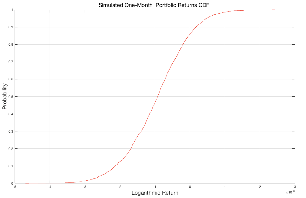
Figure 9 is a simulation of the CDF chart for one month’s market return of the carbon markets. We observe a tails dependence structure in the Chinese regional carbon emission market, and the extreme value risk in the markets is also significant. Again, we can reduce the risk of the market by constructing an appropriate portfolio.
5. Discussion
In this study, we analyze the risk of extreme value dependence in Chinese regional carbon emission markets. We first find high peaks, heavy tails and fluctuations in the logarithm returns of Chinese regional markets. The returns do not follow a normal distribution. We use a Copula model to describe the features of a dependence structure in Chinese regional markets. We find significant extreme value risk in Chinese regional markets, but the risks can be reduced by constructing an appropriate portfolio.
China established its national unified carbon emission trading market in December 2017. However, it is difficult for regional markets to be fully integrated with the national market. One reason is that the eight regional markets are located in different regions with various economic development and information infrastructure. In addition, some regional carbon emission market data have been missing since April 2018, which could result in small sample size and inaccurate parameter estimates. Therefore, we do not examine whether risk characteristics have changed around 2017. However, it is worthy to conduct further analysis on whether interdependence between regional carbon emission trading markets will change before and after the establishment of the national carbon trading market, and what changes take place when sufficient data become available.
When simulating the VaR of a portfolio, we assume the assets to be equally weighted and without transaction costs to simplify the analysis. The results indicate that the maximum simulated loss and gains both exhibit greater extreme risk. This conclusion may be affected by the weight of the portfolio asset, as asset prices have dependence when extreme events occur. Will the degree of dependence affect the risk of the investment portfolio? If the answer is yes, then these dependencies should be considered and measured when formulating investment portfolio strategies. Therefore, an introduction of the dependency parameter into the weight setting might be warranted in future research.
Our findings have important policy implications for the Chinese government and governments in other developing countries. First, China’s carbon emission trading market has been continuously developing since its inception. A mature system of energy policies, laws, and environmental regulations is the foundation for a stable and efficient carbon market. We suggest the government implements pertinent policies on low carbon economy, energy, and environment and establishes the legal status of the carbon market. Changes in economic policies and environmental regulations tend to trigger extreme risks in the carbon trading market. We recommend that the government aims to maintain a stable policy environment in the long-run and avoid excessive policy changes in the short term.
Second, market organizers and participants should focus on risk management, particularly the extreme risk of the carbon market. To do so, carbon markets need to implement a transparent trading mechanism, unify trading standards, and develop new financial products. The introduction of financial derivatives (i.e., futures and swap contracts) might be a better way to manage carbon trading risks. However, market participants should monitor trading risks closely and improve their risk management system. Developing suitable market models, measuring and predicting risk changes, and preparing for the extreme market volatility are effective ways to monitor risks in the market. Finally, a unified trading standard and effective risk monitoring require transparent and reliable data. Building credible systems for emissions measurement, data reporting, and verification is important to developing an efficient carbon trading market [50,51].
Author Contributions
H.Q.: Methodology, Software, Investigation, Funding acquisition, Writing—review and editing. G.H.: Conceptualization, Writing—original draft preparation. Y.Y.: Resources, Data curation, Supervision. J.Z.: Visualization, Resources, Software, Editing. T.Z.: Writing—review and editing, Supervision. All authors have read and agreed to the published version of the manuscript.
Funding
This research was funded by the General Program of Humanity and Social Science, Ministry of Education, grant number [16YJC790030], Anhui Natural Science Foundation, grant number [1708085QG163], the Innovation Fund of the Research Institute of International Economics and Management, Xihua University, grant number [20200011], and the Humanities & Social Sciences research projects of Ministry of Education, grant number [17YJA630121].
Acknowledgments
We thank Zhiqiang Lin at Chengdu Instrument Corporation for his valuable advice, Qian Wang at the Research Institute of International Economics and Management for editing a draft of this manuscript, and the anonymous reviewers for their valuable comments.
Conflicts of Interest
The authors declare no conflict of interest.
References
- Christoffersen, P.F. Copyright-elements of financial risk management. In Elements of Financial Risk Management; Christoffersen, P., Ed.; Elsevier: Amsterdam, The Netherlands, 2012; pp. 3–20. [Google Scholar]
- Deng, M.Z.; Zhang, W.X. Recognition and analysis of potential risks in China’s carbon emission trading markets. Adv. Clim. Chang. Res. 2019, 10, 30–46. [Google Scholar] [CrossRef]
- Subramaniam, N.; Wahyuni, D.; Cooper, B.J.; Leung, P.; Wines, G. Integration of carbon risks and opportunities in enterprise risk management systems: Evidence from Australian firms. J. Clean. Prod. 2015, 96, 407–417. [Google Scholar] [CrossRef]
- Chu, W.; Chai, S.; Chen, X.; Du, M. Does the Impact of Carbon Price Determinants Change with the Different Quantiles of Carbon Prices? Evidence from China ETS Pilots. Sustainability 2020, 12, 5581. [Google Scholar] [CrossRef]
- Grubb, M.; Neuhoff, K. Allocation and competitiveness in the EU emissions trading scheme: Policy overview. Clim. Policy 2006, 6, 7–30. [Google Scholar] [CrossRef]
- Mo, J.L.; Zhu, L.; Fan, Y. The impact of the EU ETS on the corporate value of European electricity corporations. Energy 2012, 45, 3–11. [Google Scholar] [CrossRef]
- Zhao, F.; Liu, F.; Hao, H.; Liu, Z. Carbon Emission Reduction Strategy for Energy Users in China. Sustainability 2020, 12, 6498. [Google Scholar] [CrossRef]
- Abadie, L.M.; Chamorro, J.M. European CO2 prices and carbon capture investments. Energy Econ. 2008, 30, 2992–3015. [Google Scholar]
- Hartman, P.; Straetmans, S.; De Vries, C.G. Asset market linkages in crisis periods. Rev. Econ. Stat. 2004, 86, 313–326. [Google Scholar] [CrossRef] [Green Version]
- McNeil, A.J.; Frey, R.; Embrechts, P. Quantitative Risk Management: Concepts, Techniques and Tools; Princeton University Press: Princeton, NY, USA, 2005. [Google Scholar]
- Longin, F.; Solnik, B. Extreme correlation of international equity markets. J. Financ. 2001, 56, 649–676. [Google Scholar]
- Longin, F.; Pagliardi, G. Tail relation between return and volume in the US stock market: An analysis based on extreme value theory. Econ. Lett. 2016, 145, 252–254. [Google Scholar] [CrossRef]
- Liu, G.Q.; Wei, Y.; Chen, Y.F.; Yu, J.; Hu, Y. Forecasting the value-at-risk of Chinese stock market using the HARQ model and extreme value theory. Phys. A Stat. Mech. Appl. 2018, 499, 288–297. [Google Scholar] [CrossRef]
- Sobreira, N.; Louro, R. Evaluation of volatility models for forecasting Value-at-Risk and Expected Shortfall in the Portuguese stock market. Financ. Res. Lett. 2020, 32, 101098. [Google Scholar] [CrossRef]
- Longin, F. From VaR to stress testing: The extreme value approach. J. Bank. Financ. 2000, 24, 1097–1130. [Google Scholar] [CrossRef]
- Angelidis, T.; Benos, A.; Degiannakis, S. The use of GARCH models in VaR estimation. Stat. Methodol. 2004, 1, 105–128. [Google Scholar] [CrossRef] [Green Version]
- Biage, M. Analysis of shares frequency components on daily value-at-risk in emerging and developed markets. Phys. A Stat. Mech. Appl. 2019, 532, 121798. [Google Scholar] [CrossRef]
- Hammoudeh, S.; Nguyen, K.D.; Sousa, M.R. What explains the short-term dynamics of the prices of CO2 emissions? Energy Econ. 2014, 46, 122–135. [Google Scholar] [CrossRef]
- Sklar, A. Fonctions de Répartition à n Dimensions et leurs Marges. Publ. l’Institut Stat. l’Université Paris 1959, 8, 229–231. [Google Scholar]
- Wang, Z.; Chen, X.; Jin, Y.; Zhou, Y. Estimating risk of foreign exchange portfolio: Using VaR and CVaR based on GARCH-EVT-Copula model. Phys. A Stat. Mech. Appl. 2010, 389, 4918–4928. [Google Scholar] [CrossRef]
- Berger, T. Forecasting value-at-risk using time varying copulas and EVT return distributions. Int. Econ. 2013, 133, 93–106. [Google Scholar] [CrossRef]
- Hussain, S.I.; Li, S. The dependence structure between Chinese and other major stock markets using extreme values and copulas. Int. Rev. Econ. Financ. 2017, 56, 421–437. [Google Scholar] [CrossRef]
- Herrera, R.; González, S.; Clements, A. Mutual excitation between OECD stock and oil markets: A conditional intensity extreme value approach. N. Am. J. Econ. Financ. 2018, 46, 70–88. [Google Scholar] [CrossRef]
- Jiang, J.J.; Ye, B. Value-at-Risk Estimation of Carbon Spot Market Based on the Combined GARCH-EVT-VaR Model. Adv. Mater. Res. 2014, 1065, 3250–3253. [Google Scholar] [CrossRef]
- Bedford, T.; Cooke, R.M. Probability density decomposition for conditionally dependent random variables modeled by vines. Ann. Math. Artif. Intell. 2001, 32, 245–268. [Google Scholar] [CrossRef]
- Bedford, T.; Cooke, R.M. Vines-A new graphical model for dependent random variables. Ann. Stat. 2002, 30, 1031–1068. [Google Scholar] [CrossRef]
- Dißmann, J.; Brechmann, E.C.; Czado, C.; Kurowicka, D. Selecting and estimating regular vine copula and application to financial returns. Comput. Stat. Data Anal. 2013, 59, 52–69. [Google Scholar] [CrossRef] [Green Version]
- Koliai, L. Extreme risk modeling: An EVT-Pair-copulas approach for financial stress tests. J. Bank. Financ. 2016, 70, 1–22. [Google Scholar] [CrossRef]
- Feng, Z.; Wei, Y.; Wang, K. Estimating risk for the carbon market via extreme value theory: An empirical analysis of the EU ETS. Appl. Energy 2012, 99, 97–108. [Google Scholar] [CrossRef]
- Philip, D.; Shi, Y. Optimal hedging in carbon emission markets using Markov regime switching models. J. Int. Financ. Mark. Inst. Money 2016, 43, 1–15. [Google Scholar] [CrossRef] [Green Version]
- Boyce, J.K. Carbon pricing: Effectiveness and equity. Ecol. Econ. 2018, 150, 52–61. [Google Scholar] [CrossRef]
- Jiao, L.; Liao, Y.; Zhou, Q. Predicting carbon market risk using information from macroeconomic fundamentals. Energy Econ. 2018, 73, 212–227. [Google Scholar] [CrossRef]
- Zhu, J.M.; Wu, P.; Chen, H.Y.; Liu, J.P.; Zhou, L.G. Carbon price forecasting with variational mode decomposition and optimal combined model. Phys. A Stat. Mech. Appl. 2018, 519, 140–158. [Google Scholar]
- Chang, K.; Pei, P.; Zhang, C.; Wu, X. Exploring the price dynamics of CO2 emission allowances in China’s emissions trading scheme pilots. Energy Econ. 2017, 67, 213–223. [Google Scholar]
- Yin, Y.; Jiang, Z.; Liu, Y.; Yu, Z. Factors Affecting Carbon Emission Trading Price: Evidence from China. Emerg. Mark. Financ. Trade 2019, 55, 3433–3451. [Google Scholar]
- Dai, Y.; Li, N.; Gu, R.; Zhu, X. Can China’s Carbon Emissions Trading Rights Mechanism Transform its Manufacturing Industry? Based on the Perspective of Enterprise Behavior. Sustainability 2018, 10, 2421. [Google Scholar]
- Ramazan, G.; Faruk, S.; Ulugülyaǧci, A. High volatility, thick tails and extreme value theory in value-at-risk estimation. Insur. Math. Econ. 2003, 33, 337–356. [Google Scholar]
- Bollerslev, T. Generalized autoregressive conditional heteroscedasticity. J. Econom. 1986, 31, 307–327. [Google Scholar]
- Gazola, L.; Fernandes, C.; Pizzinga, A. The log-periodic-AR(1)-GARCH(1,1) model for financial crashes. Eur. Phys. J. B 2008, 61, 355–362. [Google Scholar]
- Richard, P.; Kabin, K. GARCH (1,1) model of the financial market with the Minkowski metric. Ztschrift Nat. A 2018, 73, 669–684. [Google Scholar]
- Mika, M.; Pentti, S. Stability of nonlinear AR-GARCH models. J. Time Ser. Anal. 2008, 29, 453–475. [Google Scholar]
- Peng-Cheng, M.A.; Sha-Sha, W.U.; Zhen-Fang, H. SHIBOR Rate Fluctuations Based on AR(1)-GARCH(1,1) Model. J. Hebei North Univ. Nat. Sci. Ed. 2012, 28, 1–5. [Google Scholar]
- Scarrott, C.; MacDonald, A. A reviewof extreme value threshold estimation and uncertainty quantification. Stat. J. 2012, 10, 33–60. [Google Scholar]
- DuMouchel, W.H. Estimating the table index α in order to measure tail thickness: A critique. Ann. Stat. 1983, 11, 1019–1031. [Google Scholar] [CrossRef]
- Boyer, B.H.; Gibson, M.S.; Loretan, M. Pitfalls in Tests for Changes in Correlations. 1997. Available online: https://ssrn.com/abstract=58460 (accessed on 18 July 2020).
- Patton, A.J. Skewness, Asymmetric Dependence, and Portfolios; London School of Economics & Political Science: London, UK, 2002; Working paper of London School of Economics & Political Science. [Google Scholar]
- Cuculescu, I.; Theodorescu, R. Extreme value attractors for star unimodal copulas. Comptes Rendus Math. 2002, 334, 689–692. [Google Scholar] [CrossRef]
- Hürlimann, W. Hutchinson-Lai’s conjecture for bivariate extreme value copulas. Stat. Probab. Lett. 2003, 61, 191–198. [Google Scholar] [CrossRef]
- Rosenberg, J.V.; Schuermann, T. A general approach to integrated risk management with skewed, fat-tailed risks. J. Financ. Econ. 2004, 79, 569–614. [Google Scholar] [CrossRef] [Green Version]
- Vermillion, S. Lessons from China’s Carbon markets for U.S. climate change policy. William Mary Environ. Law Policy Rev. 2015, 39, 457–482. [Google Scholar]
- Zhang, D.; Zhang, Q.; Qi, S.; Huang, J.; Karplus, V.; Zhang, X. Integrity of firms’ emissions reporting in China’s early carbon markets. Nat. Clim. Chang. 2019, 9, 164–169. [Google Scholar] [CrossRef]
Figure 1.
The daily index of the six regional Carbon emission trading markets, and the figure plots the daily index of the six regional Carbon emission trading markets for the whole sample period of April 1, 2014 to April 12, 2018. It consists of 1134 daily observations after deleting the missing data and the data without a corresponding trading day. The source is from TANKQIAM (http://k.tanjiaoyi.com/).

Figure 2.
Normal Q-Q plot of the daily logarithm returns for each regional carbon emission trading market. HB, BJ, SH, GZ, TJ, and SZ respectively represent the carbon emission markets of Hubei, Beijing, Shanghai, Guangzhou, Tianjin, and Shenzhen. It is shown that the curves exist as tails, which means the data have more extreme values than would be expected. This indicates that it is misaligned with normal distribution.
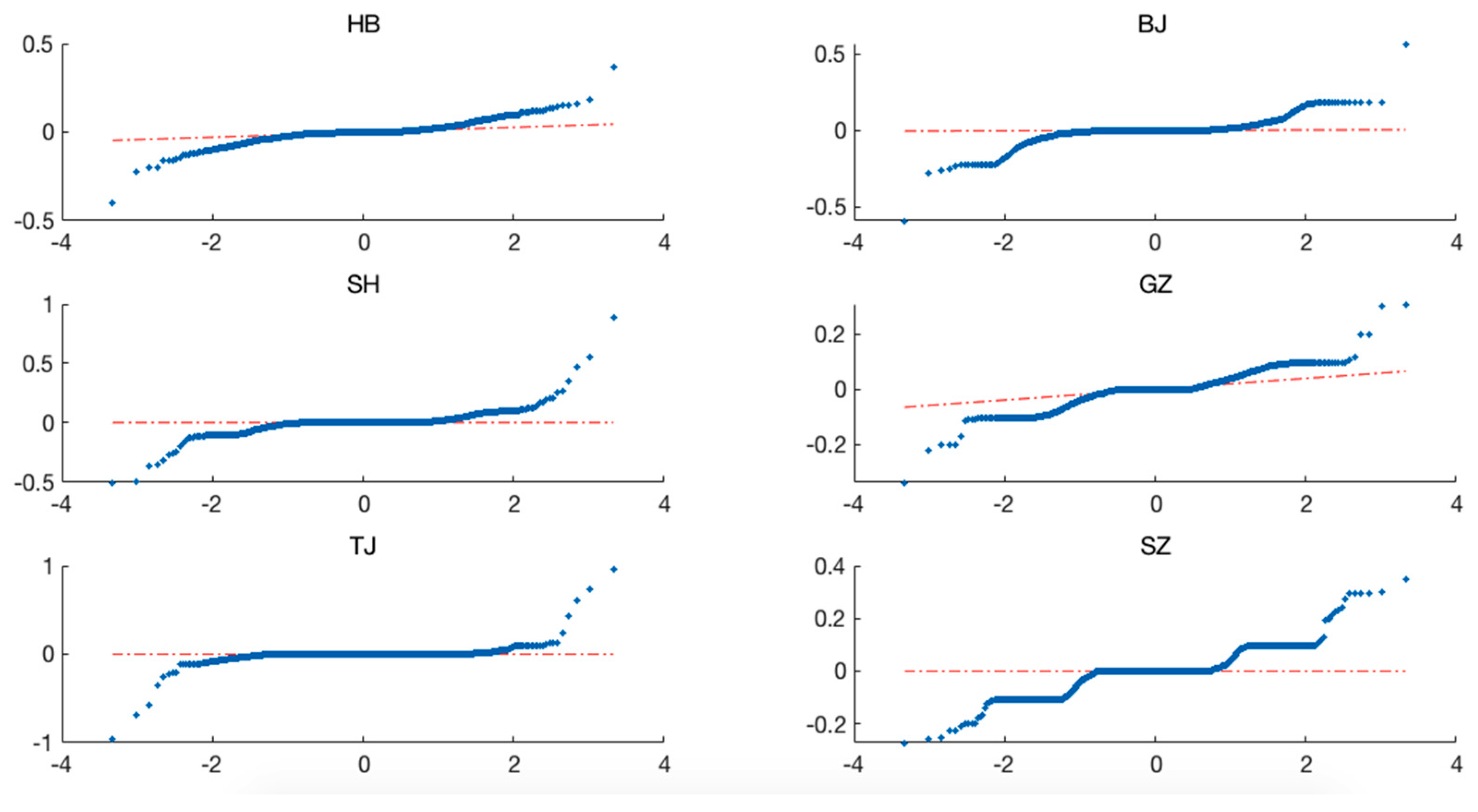
Figure 3.
Daily logarithmic returns of the six regional carbon emission trading markets from the period of April 1, 2014 to April 12, 2018. HB, BJ, SH, GZ, TJ, and SZ respectively represent the carbon emission markets of Hubei, Beijing, Shanghai, Guangzhou, Tianjin, and Shenzhen. The figure provides the evidence of volatility clustering in the returns of the six markets.
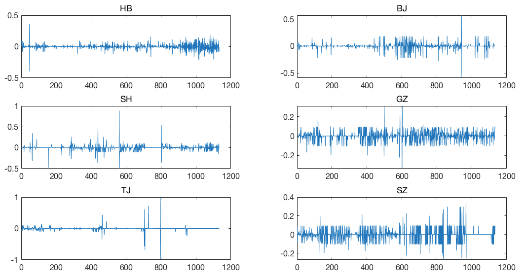
Figure 4.
Autocorrelation functions (ACF) of returns in the six markets. HB, BJ, SH, GZ, TJ, and SZ respectively represent the carbon emission markets of Hubei, Beijing, Shanghai, Guangzhou, Tianjin, and Shenzhen. The figure reveals some mild serial correlations in the markets.
Figure 4.
Autocorrelation functions (ACF) of returns in the six markets. HB, BJ, SH, GZ, TJ, and SZ respectively represent the carbon emission markets of Hubei, Beijing, Shanghai, Guangzhou, Tianjin, and Shenzhen. The figure reveals some mild serial correlations in the markets.
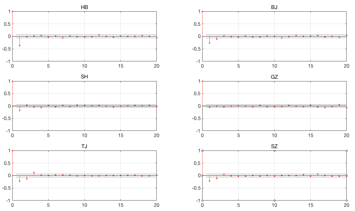
Figure 5.
Autocorrelation functions (ACF) of the squared returns in the six regional markets. HB, BJ, SH, GZ, TJ, and SZ respectively represent the carbon emission markets of Hubei, Beijing, Shanghai, Guangzhou, Tianjin, and Shenzhen. The figure reveals the degree of persistence in variance and implies that GARCH models could be used in fitting the characteristics of the returns.
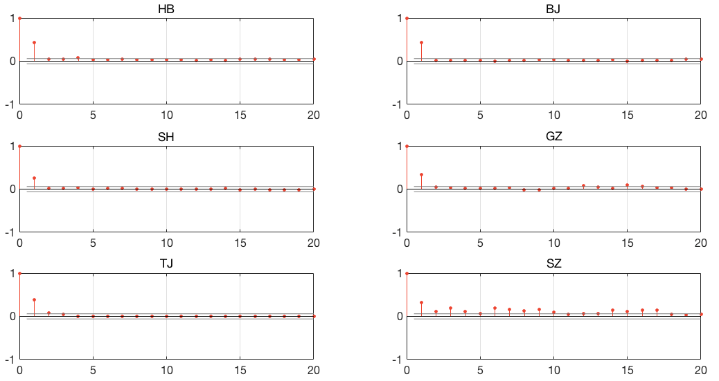
Figure 6.
Autocorrelation functions (ACF) of the standardized residuals in the six regional markets. HB, BJ, SH, GZ, TJ, and SZ respectively represent the carbon emission markets of Hubei, Beijing, Shanghai, Guangzhou, Tianjin, and Shenzhen. The figure reveals that the standardized residuals are now approximately i.i.d.
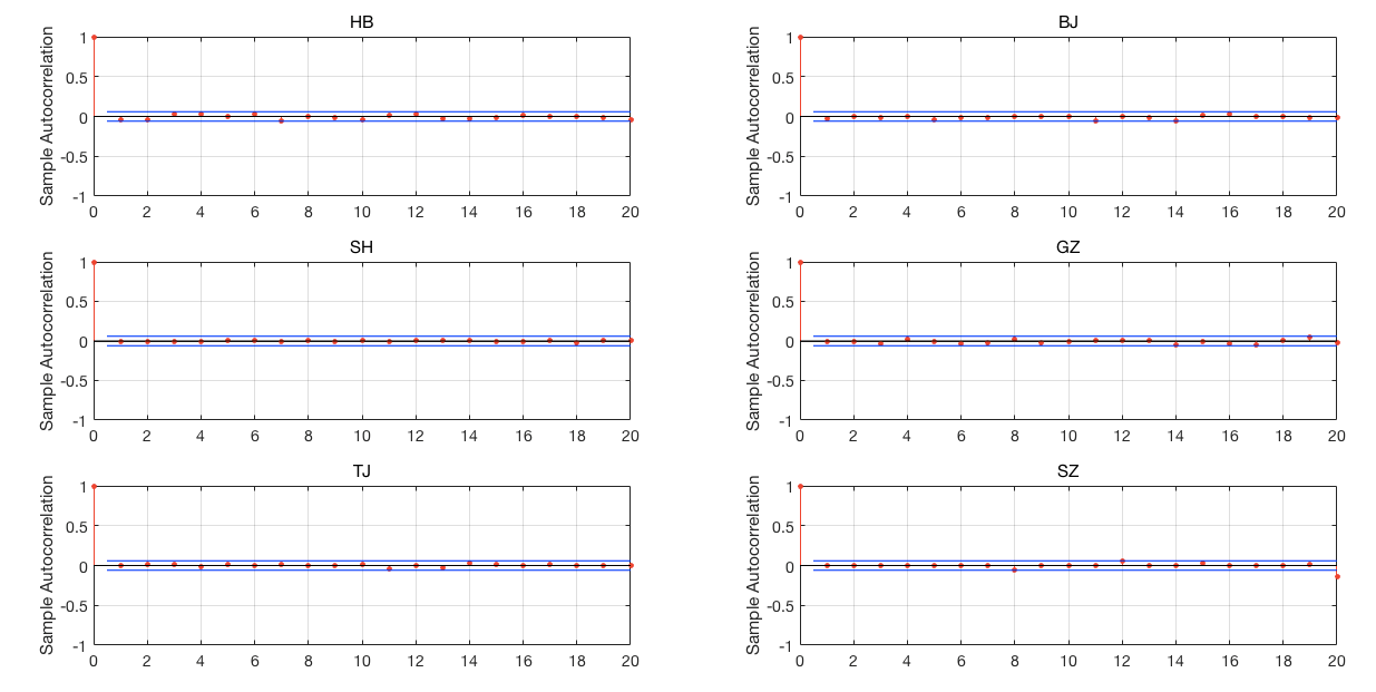
Figure 7.
Cumulative Distribution Function (CDF) of the exceedance of the residuals, along with the CDF from GPD for the six regional markets. HB, BJ, SH, GZ, TJ, and SZ respectively represent the carbon emission markets of Hubei, Beijing, Shanghai, Guangzhou, Tianjin, and Shenzhen. These Pareto tails show the estimates of the parametric generalized Pareto lower tail, the non-parametric kernel-smoothed interior, and the parametric generalized Pareto upper tail, to build a composite semi-parametric CDF for the residuals. The lower and upper tail regions are respectively displayed in red and blue, while the kernel-smoothed interior is black.

Figure 8.
Cumulative Distribution Function (CDF) of the exceedance of the residuals for the upper tail, along with the CDF from GPD for the six regional markets. HB, BJ, SH, GZ, TJ and SZ respectively represent the carbon emission markets of Hubei, Beijing, Shanghai, Guangzhou, Tianjin and Shenzhen. The fitted generalized Pareto CDF and empirical CDF are respectively displayed in blue and red. 10% of the standardized residuals are used, and the fitted distribution is closely following the most exceedance data.
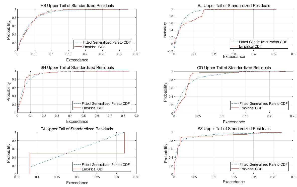
Figure 9.
Description of simulated one-month portfolio returns CDF.

Table 1.
Descriptive statistics of daily log-returns.
| HB | BJ | SH | GZ | TJ | SZ | |
|---|---|---|---|---|---|---|
| Mean | −0.0004 | 0 | 0 | −0.0012 | −0.0012 | −0.0005 |
| Std. | 0.043 | 0.0581 | 0.063 | 0.0515 | 0.0646 | 0.0634 |
| Kurtosis | 16.8556 | 25.3499 | 55.4872 | 7.6041 | 131.0534 | 7.2871 |
| Skewness | −0.3211 | −0.6705 | 2.1326 | −0.1766 | 0.3916 | 0.3409 |
| Jarque-Box | 9082.4 | 23666 | 130910 | 1006.6 | 77414 | 889.5997 |
HB, BJ, SH, GZ, TJ, and SZ respectively represent the carbon emission markets of Hubei, Beijing, Shanghai, Guangzhou, Tianjin, and Shenzhen. Jarque-Box denotes the statistics of the Jarque-Bera normality test at a 5% level. The sample period is from 1 April 2014 to 12 April 2018.
Table 2.
A Monte Carlo simulation of portfolio asset returns.
| Freedom | Maximum Simulated Loss | Maximum Simulated Revenue | VaR | ||
|---|---|---|---|---|---|
| 90% | 95% | 99% | |||
| 23.1829 | 0.4689% | 0.2437% | −0.2141% | −0.2486% | −0.3116% |
This table reports the maximum gain and loss, and estimates of the Value-at-Risk with confidence levels of 90%, 95% and 99% for an asset portfolio of Carbon financial assets over a one-month risk horizon of 22 trading days. The weight of each asset in the portfolio is equal, and the portfolio weights are held fixed throughout the risk horizon. The method is the Monte Carlo simulation method.
© 2020 by the authors. Licensee MDPI, Basel, Switzerland. This article is an open access article distributed under the terms and conditions of the Creative Commons Attribution (CC BY) license (http://creativecommons.org/licenses/by/4.0/).
Share and Cite
MDPI and ACS Style
Qiu, H.; Hu, G.; Yang, Y.; Zhang, J.; Zhang, T. Modeling the Risk of Extreme Value Dependence in Chinese Regional Carbon Emission Markets. Sustainability 2020, 12, 7911. https://doi.org/10.3390/su12197911
AMA Style
Qiu H, Hu G, Yang Y, Zhang J, Zhang T. Modeling the Risk of Extreme Value Dependence in Chinese Regional Carbon Emission Markets. Sustainability. 2020; 12(19):7911. https://doi.org/10.3390/su12197911
Chicago/Turabian StyleQiu, Hong, Genhua Hu, Yuhong Yang, Jeffrey Zhang, and Ting Zhang. 2020. "Modeling the Risk of Extreme Value Dependence in Chinese Regional Carbon Emission Markets" Sustainability 12, no. 19: 7911. https://doi.org/10.3390/su12197911
Note that from the first issue of 2016, this journal uses article numbers instead of page numbers. See further details here.