A Novel Closed-Loop Supply Chain Network Design Considering Enterprise Profit and Service Level

Abstract

Increasing concerns for sustainable development have motivated the study of closed-loop supply chain network design from a multidimensional perspective. To cope with such issues, this paper presents a general closed-loop supply chain network comprising various recovery options and further formulates a multi-objective mixed-integer linear programming model considering enterprise profit and service level simultaneously. Within this model, market segmentation is also considered to meet real-world operating conditions. Moreover, an $\epsilon$-constraint method and two interactive fuzzy approaches are applied to find a global optimum for this model together with the decisions on the numbers, locations, and capacities of the facilities, as well as the material flow through the network. Ultimately, numerical experiments are conducted to demonstrate the viability and effectiveness of both the proposed model and solution approaches.

1. Introduction

During the last few decades, great attention has been paid to the practice of collecting and reusing used up products, involving almost all of the manufacturing industries [1]. The reasons for these interests can be attributed to environmental and economic factors. The former includes the used items’ environmental impacts, the governmental legislation, the customers’ environmental awareness, and the waste pollution. Among them, the government develops important functions for promoting the implementation of product returns, especially by law enforcement (e.g., the Waste Electrical and Electronic Equipment and End-of-life Vehicles directives of the EU) [2]. The latter involves the returns’ economical advantages, improving customer satisfaction, reducing costs, and adding value to the logistics network. In practice, many companies, such as Dell, General Motors, and Hewlett-Packard, have achieved great success through recovery activities [3]. Obviously, effectively managing the used up products has become a necessary issue that cannot be neglected in designing a supply chain.

Generally, traditional supply chain network design refers to the forward materials’ and products’ flow encompassing a series of processes with information and money (financial) flows going backward and the ultimate goal of maximizing the whole chain’s profits. These processes include entities like suppliers, manufactures, distributors, and customers, as usual. While considering the integration of the end-of-use products’ management and the classic supply chain, an additional backward flow, namely reverse logistics (RL), is essential to the material’s circulation from the end customers towards possible recovery entities. Thus, the closed-loop supply chain (CLSC) is generated with the consideration of both forward and reverse product flows in a supply chain simultaneously. In reality, such a configuration gains much competitive edge [4] with respect to the enterprise’s green image and resource savings. Furthermore, it makes a huge contribution to the investigation of the sustainable supply chain [5].

A CLSC network design is suitable for the durable products with features of a modular structure and a long life cycle (e.g., household appliances, automobiles), as well as the technology products characterized by a complicated function and a quick product replacement (e.g., mobile phones, laptops), when their consumption tends to cause the unacceptable waste of resources and sever environmental pollution [6]. In the backward flow, the returned products may be treated by multiple recovery alternatives, as the reverse logistics activities can help capture the remaining value in the returns collected from the end-users [7,8]. Specifically, based on the different quality of the returned items, the possible recovery options can be determined by detecting and sorting. In general, recycling is the most used option, when the returns are beneficial and there is no harm to the environment. Otherwise, they can be disposed through landfill or other suitable treatments in an environmentally sustainable way. Besides, if the returned items can be resold by remanufacturing or simple repair, the recovered products can be redistributed to the secondary market. Due to the difference in quality between the remanufactured items and the newly produced items, different markets (i.e., the primary market and the secondary market) with different prices also need to be considered.

On the other hand, compared with the CLSC network design only considering a single objective (usually attempting to minimize cost or maximize profit), multi-objective optimization is more reasonable and practical in terms of actual applications [9]. Among other traditional measures of the supply chain operation performance, customer satisfaction is one of the key factors in getting a sustainable competitive advantage in today’s business environment. Undoubtedly, to gain customer satisfaction, a high level of service should be offered to the customers. Generally, as for the supply chain operations, the service level can be measured by the fill rate, which refers to the fraction or amount of customer demands satisfied within the promised delivery time [10]. Therefore, in order to promote and maintain the competitive superiority of enterprises for long term development, the customer service level involving the delivery time should also be taken into account.

Based on the aforementioned considerations, this paper addresses the issue of multi-objective and multi-echelon supply chain network design, including manufactures, distribution centers, customer zones, disassembly centers (collection/inspection centers), redistribution centers, and disposal centers in the network. In this model, we not only incorporate the forward and reverse logistics in a general CLSC model, but also embed multiple recovery options as a distinct decision differing from the simply recycling-or-dispose choice. Additionally, the $\epsilon$-constraint method and two interactive fuzzy approaches are applied to find Pareto-optional solutions of the multi-objective CLSC network design problem, and specific analyses of these solution approaches, as well as the effect of some important parameters on the optimal solution, objective function values, and network configuration are presented.

The remainder of this paper is organized as follows. Section 2 presents an overview of the most relevant literature and outlines the main contributions. Section 3 describes more details of the CLSC network design problem investigated in this paper, which is formulated as a multi-objective programming model in Section 4. Subsequently, Section 5 introduces the solution approaches to the programming model. Numerical experiments are reported in Section 6, and finally, conclusions are given in Section 7.

2. Literature Review

Since the concept of RL was proposed by Stock in 1992, the supply chain network with reverse recovery has received increasing attention. While the traditional, one way logistic model easily leads to sub-optimalities from the separated configuration [11], Fleischmann et al. [12] integrated the forward and reverse flows in a supply chain simultaneously as early as 2001, offering a commonly used quantitative mixed-integer linear programming model (MILP) for the CLSC design. After that, many authors, like Sahyouni, Savaskan, and Daskin [13] and Lee, Dong, and Bian [14], further demonstrated the efficiency and effectiveness of the integrated approach compared to a sequential approach. Most of these studies commonly investigated the network echelons, facilities, recovery options, as well as optimization methods of the proposed network design problems. In what follows, we present a more detailed analysis of the related work that takes into account multiple recovery options and multi-objective network design problems and then present the main contributions of this paper.

2.1. RL and CLSC Network Design with Multiple Recovery Options

In recent decades, the majority of relevant papers were about the RL and CLSC network design focusing on the remanufacturing or recycling option for all returned products (e.g., [15,16]), due to the obvious economic and ecological benefits obtained from the circular economy. Aras, Aksen, and Gonul Tanugur [7] pointed out that both remanufacturing and recycling activities can help reduce the unit cost of production by 40–60%. Wang et al. [17] established a system dynamic model to test and verify the mixed-subsidy policies’ positive effects on these two treatments. Besides, there is also a number of papers covering other different recovery alternatives. In 2006, Kannan, Sasikumar, and Devika [18] developed a CLSC model for the case of battery recycling with multiple recovery options, which consisted of repair, remanufacture, raw material recycling, and waste disposal, aiming at minimizing the supply chain costs. Based on the different ways of treating the various returns, El-Sayed, Afia, and El-Kharbotly [19] further differentiated the demand market for new products from the used products to capture the realistic situations. On account of the profitable value recovery from the returned items, Alumur et al. [20] presented a general MILP formulation incorporating several means of tackling these returns in an RL network design, such as recycling, external remanufacturing, and the secondary market. A case study of large household appliances verified the effectiveness of the proposed model. Furthermore, the effect of the return rate was investigated, showing that the total expected profit increased with the increase of the return rate.

Considering whether the rate of each recovery option was varied or fixed, many models were proposed with a fixed recovery rate per option (e.g., [21,22,23,24]), whereas a few models considered the variation of proportions of products assigned to every recovery option. For example, Krikke, Bloemhof-Ruwaard, and Van Wassenhove [25] constructed a CLSC network model with cost minimization in which the returned products could be reused or remanufactured in modules or components instead of the virgin materials. A “feasibility rate” was provided for each option, which restricted the recovery rate per option within a given limit. Then, the authors performed a sensitivity analysis to investigate the impact of the varying rate of return, recovery feasibility, and recovery targets on the product cost. Ozkir and Basligil [26] presented another sensitivity analysis for a capacitated CLSC model incorporating three product recovery alternatives. They studied the impact of varying return rates and return quality showing that the return rate variation had more significant influence on the total profit than the return quality did. Recently, Jerbia et al. [27] investigated a stochastic CLSC network design model with multiple recovery options, where they explored the changes of the network structure and the total profitability when the main parameters (i.e., return rates, revenues, costs and quality of return) of the model varied.

2.2. RL and CLSC Network Design with Multiple Objectives

In RL and CLSC network design, multi-objective programming models have been studied by many researchers in recent years. On the basis of the usual economic indicators (e.g., minimum cost, maximum profit), some papers considered sustainability, the enterprise’s social responsibility, customer service level, and others as additional objectives.

Prior to the sustainable supply chain network design, studies mainly focused on the economic and financial business performance in the early stage. With the enrichment of sustainability theory, the environmental and social impacts of supply chain operations, as well as the economic benefits began to be considered in the multi-objective network design problems. For instance, Ozkir and Basligil [28] established a CLSC model considering three recovery options and deduced three levels of objective functions relating to profit maximization, trade satisfaction, and customer satisfaction. Talaei et al. [29] investigated the remanufacturing issue in a closed-loop green supply chain network design and proposed a bi-objective model considering reducing total costs and the rate of CO${}_2$ emission. The applicability of their model and the effectiveness of the solution method were illustrated via an application in the electronics industry. Furthermore, Devika et al. [5] emphasized the economic performance and environmental, as well as social impacts in the model construction simultaneously, which aimed to capture the trade-off between three pillars of sustainability. In regards to the complexity of the model, they further developed competitive algorithms integrating a variable neighborhood search to solve it. Focusing on the notions of sustainable and green supply chains, Soleimani et al. [30] extended the multi-objective model of Ozkir and Basligil [28] by appending the reduction of CO${}_2$ emissions and lost working days. Besides, Masoudipour et al. [31] developed a novel multi-objective model in which total costs, CO${}_2$ emissions, and the quality of returned products were taken into account.

Except for the economic and sustainable objectives, a good network design would also help the enterprise accelerate its operation efficiency and further improve the customer satisfaction level, which ultimately benefits the enterprise. Hence, there is a growing trend to regard customer service level as an important measurable goal [32]. Generally, this goal can be measured via the delayed delivery time, responsiveness rate, defective products’ rate, and others. For example, Pishvaee and Torabi [33] proposed a structure to model a CLSC network with costs and service level considerations and presented an efficient interactive fuzzy approach to minimize the total costs and tardiness of delivered products. Since the quicker the network responsiveness, the higher the customer satisfaction, Khajavi et al. [34] investigated the integrated forward/reverse logistics network and presented a bi-objective mixed-integer programming model, in which the minimization of costs and maximization of the network responsiveness were taken into account. For the long lasting efficient operation of the entire supply chain, Ramezani et al. [10] designed a stochastic multi-objective model for a forward/reverse supply chain network, considering the maximization of profit and responsiveness and the minimization of defective parts delivered from suppliers.

2.3. Main Contributions

As stated above, most of the literature on RL and CLSC network design considers only one or two recovery options for returned items, such as Guide and Danial [15], Dowlatshahi [16], and so on. Just a few papers that we surveyed in our literature review took into account multiple recovery options. However, among of them, some papers constructed models for some particular products (e.g., [18,22]), which lacked generality. Besides, the separated design of the forward and reverse chains easily resulted in sub-optimalities (e.g., [20]). Hence, our paper comes to enrich this stream of literature by presenting a general CLSC network design model including repair, recycling, remanufacturing, redistributing, and disposal. Furthermore, the model also considers the secondary markets for the remanufactured products. Additionally, while the promotion of operational efficiency can improve the service level for each customer and the economic value for every enterprise, the objective function of the proposed MILP model is to maximize the enterprise profit and customer service level simultaneously. This was rare in the above mentioned studies, where many papers focused on a single objective in the research for multiple options (e.g., [19,25,26,27]) or the measurement of CO${}_2$ emissions for the sustainable multi-objective investigation (e.g., [29,30,31]). Up to now, to the best of our knowledge, there is no such paper that has designed such a network programming model with all the situations taken into account at the same time.

On the other hand, considering the multi-objective programming model proposed in this paper, we aim to adopt various effective and well behaved solution methods to solve this problem and offer much more flexible recommendations to decision makers. In the aforementioned papers, which concentrated on multi-objective investigations, most of them only utilized a single method (e.g., [29,31,34]). However, in this paper, we use the $\epsilon$-constraint method and two interactive fuzzy methods to solve the proposed model. Furthermore, similarities and differences among those multi-objective methodologies are discussed and analyzed theoretically, and they are tested in the experiments. Regarding the impact of the return rate, which had recently been emphasized by researchers (e.g., [25,26,27]), we give a thorough analysis of the return rate in the end.

3. Problem Definition

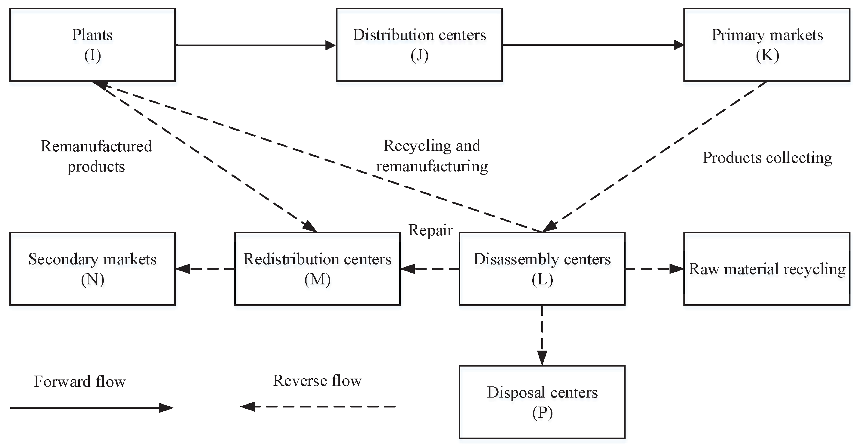
The CLSC network design problem discussed in this paper is an integrated multi-stage logistics network including three echelons in the forward direction (i.e., production/remanufacturing centers, distribution centers, primary markets) and four echelons in the backward direction (i.e., disassembly centers, redistribution centers, disposal centers, secondary markets), as illustrated in Figure 1. In the forward flow, new products are shipped from production centers to primary markets (customers of primary markets consuming the original products) through distribution centers to meet the demand of each customer. In the reverse flow, firstly, returned products collected from the primary markets are sent to disassembly centers, and then, they are tested/classified to determine the specific recovery options: (i) sent to the secondary markets (customers of secondary markets consuming remanufactured/repaired products) by the redistribution centers after simple repair for the slightly damaged products; (ii) delivered to the plants for remanufacturing for the partly available products and then sent to the secondary markets finally; (iii) recovered as raw materials for the partly recycled products; (iv) disposed by the disposal centers for the completely non-valuable products. In this model, production centers are also used for remanufacturing products. The proposed network incorporates the multiple treatment approaches that can make the best use of the returned products. To fulfill the real-life scenario, market segmentation divided by product nature is also considered.

Therefore, the network studied in this paper is a general CLSC network combining manufacture-repair-remanufacture and resource recycling into one, which can be applied to the automotive, electronics, and other consumer product industries, involving relevant enterprises like electrical equipment manufacturers, automotive parts makers, and so on.

Given the aforementioned network configuration, the CLSC design model is to determine the numbers and locations of these five types of facilities, namely plants, distribution centers, disassembly centers, redistribution centers, and disposal centers, and allocate shipped quantities of products between these facilities. Moreover, the network design of this paper is obligated to adhere to the principles of economy and efficacy, which are devoted to helping companies perfect the supply chain management and reduce energy consumption, as well as waste disposal. In this way, we aim to maximize the total profit of the enterprise through sales and recovery activities and maximize the service level through the highly efficient network operation.

The assumptions made for the problem formulation are as follows:

• A single product and single period are considered in this CLSC network design.
• Given that the quality of remanufactured and repaired products is different from the new ones, they should be sold in different markets at different prices. The new and remanufactured/repaired products correspond to the primary and secondary markets, respectively.
• Customer locations are fixed, and customer demands are known, among which the demand in primary markets must be satisfied, while the secondary markets’ may not be totally satisfied.
• On account of the products available for collecting being limited, the maximum rate of return is predetermined.
• In the four recovery options, the rate of simple repairs and the disposal rate of returns are predetermined.
• There is no flow between the facilities of the same echelon.
• Considering the instability of the recycling of waste products, the primary market customer service level is studied only.
• The capacity of each facility is restricted.

Based on the above foundational assumptions, the problem studied in this paper can be defined as a single period and single product multi-objective CLSC network design problem with multiple recovery alternatives under the capacity restrictions.

4. Model Formulation

As the problem definition stated in Section 3, in this section, the CLSC network design problem is formulated as a novel multi-objective mixed-integer linear programming (MOMILP) model. Firstly, the sets, parameters, and decision variables of the problem are introduced, and then, the model’s objective functions and constraints are explained specifically.

The model involves the following sets, parameters, and decision variables:

Sets
I	Set of potential locations of plants, ($i=\{1,2,\cdots ,I\}$);
J	Set of potential locations of distributions, ($j=\{1,2,\cdots ,J\}$);
K	Set of primary markets, ($k=\{1,2,\cdots ,K\}$);
L	Set of potential locations of disassembly, ($l=\{1,2,\cdots ,L\}$);
M	Set of potential locations of redistributions, ($m=\{1,2,\cdots ,M\}$);
N	Set of secondary markets, ($n=\{1,2,\cdots ,N\}$);
P	Set of potential locations of disposal, ($p=\{1,2,\cdots ,P\}$);
Parameters
$d_k$	Demand of customer k from the primary market;
$d_n$	Demand of customer n from the secondary market;
$f_i$	Fixed establishing cost of plant i;
$f_j$	Fixed establishing cost of distribution center j;
$f_l$	Fixed establishing cost of disassembly center l;
$f_m$	Fixed establishing cost of redistribution center m;
$f_p$	Fixed establishing cost of disposal center p;
$p_i$	Capacity of plant i;
$p_j$	Capacity of distribution center j;
$p_l$	Capacity of disassembly center l;
$p_m$	Capacity of redistribution center m;
$p_p$	Capacity of disposal center p;
$t{c}_{ij}$	Unit transportation cost from plant i to distribution center j;
$t{c}_{jk}$	Unit transportation cost from distribution center j to customer k;
$t{c}_{li}$	Unit transportation cost from disassembly center l to plant i;
$t{c}_{lm}$	Unit transportation cost from disassembly center l to redistribution center m;
$t{c}_{lp}$	Unit transportation cost from disassembly center l to disposal center p;
$t{c}_{im}$	Unit transportation cost from plant i to redistribution center m;
$t{c}_{mn}$	Unit transportation cost from redistribution center m to customer n;
$t{c}_{lp}$	Unit transportation cost from disassembly center l to disposal center p;
$t{c}_{im}$	Unit transportation cost from plant i to redistribution center m;
$t{c}_{mn}$	Unit transportation cost from redistribution center m to customer n;
$v{c}_i$	Unit remanufacturing cost at plant i;
$r{c}_l$	Unit repairing cost at disassembly center l;
$d{c}_p$	Unit disposal cost at disposal center p;
$h{c}_j$	Unit treatment cost at distribution center j;
$h{c}_l$	Unit treatment cost at disassembly center l;
$h{c}_m$	Unit treatment cost at redistribution center m;
$m{c}_i$	Unit manufacturing cost at plant i;
$c{c}_{kl}$	Unit recovery cost of used product from customer k to disassembly center l;
$\omega$	Maximum recovery ratio of used product;
${\theta }_1$	Disposal ratio;
${\theta }_2$	Repairing ratio;
$d{t}_{jk}$	Delivery time from distribution center j to customer k;
$e{t}_k$	Expected delivery time of customer k;
$s_1$	Unit income of new product;
$s_2$	Unit income of remanufactured product;
$s_3$	Unit recovery income of raw material;
Decision variables
$X_{ij}$	Flow of product from plant i to distribution center j;
$X_{jk}$	Flow of product from distribution center j to customer k;
$X_{kl}$	Flow of returned product from customer k to disassembly center l;
$X_{li}$	Flow of recoverable product from disassembly center l to plant i;
$X_{lm}$	Flow of repaired product from disassembly center l to redistribution center m;
$X_{lp}$	Flow of scrapped product from disassembly center l to disposal center p;
$X_{im}$	Flow of remanufactured product from plant i to redistribution center m;
$X_{mn}$	Flow of repaired product and remanufactured product from redistribution center m to second customer n;
$X_l$	Flow of raw material from disassembly center l to suppliers;
$Y_i$	Binary variable equal to 1 if plant i is open and 0 otherwise;
$Y_j$	Binary variable equal to 1 if distribution center j is open and 0 otherwise;
$Y_l$	Binary variable equal to 1 if disassembly center l is open and 0 otherwise;
$Y_m$	Binary variable equal to 1 if redistribution center m is open and 0 otherwise;
$Y_p$	Binary variable equal to 1 if disposal center p is open and 0 otherwise.

In terms of the above mentioned notations, the multi-objective CLSC network design problem can be formulated as follows.

4.1. Objective Functions

4.1.1. Objective Function 1: Maximizing the Enterprise Profit

The first objective function is to maximize the total profit, which can be calculated by the total sales revenue minus total costs.

• Total sales revenue:

Based on the functions and activities of each entity in the supply chain, the total sales revenue of the network includes the new product sales, the remanufactured product sales, and the recovery income of raw material sales. Hence, the total sales revenue $TS$ is calculated as follows:

$$TS=\sum _{j\in J}\sum _{k\in K}{s}_1{X}_{jk}+\sum _{m\in M}\sum _{n\in N}{s}_2{X}_{mn}+\sum _{l\in L}{s}_3{X}_l.$$

(1)

• Total costs:

Two types of costs are considered in the CLSC network design, i.e., fixed costs of establishing and operating these facilities and variable operation costs that depend on the volumes of products to be handled. Specifically, the fixed cost $FC$ and various variable operation costs, including transportation costs $TC$, manufacturing costs $MC$, treatment costs $HC$, recovery costs $CC$, remanufacturing costs $RMC$, repairing costs $RC$, and disposal costs $DC$, are formulated by Equations (2)–(9), respectively. Note that since almost all costs can be divided into these two types, fixed or variable costs, in terms of whether they change with the volumes being processed, other costs not being considered in this study can be similarly treated in our proposed model and solution approaches.

$$FC=\sum _{i\in I}{f}_i{Y}_i+\sum _{j\in J}{f}_j{Y}_j+\sum _{l\in L}{f}_l{Y}_l+\sum _{m\in M}{f}_m{Y}_m+\sum _{p\in P}{f}_p{Y}_p$$

(2)

$$\begin{array}{c}{\displaystyle TC=\sum _{i\in I}\sum _{j\in J}t{c}_{ij}{X}_{ij}+\sum _{j\in J}\sum _{k\in K}t{c}_{jk}{X}_{jk}+\sum _{l\in L}\sum _{i\in I}t{c}_{li}{X}_{li}+\sum _{l\in L}\sum _{m\in M}t{c}_{lm}{X}_{lm}}\hfill \\ {\displaystyle +\sum _{l\in L}\sum _{p\in P}t{c}_{lp}{X}_{lp}+\sum _{i\in I}\sum _{m\in M}t{c}_{im}{X}_{im}+\sum _{m\in M}\sum _{n\in N}t{c}_{mn}{X}_{mn}}\hfill \end{array}$$

(3)

$$MC=\sum _{i\in I}\sum _{j\in J}m{c}_i{X}_{ij}$$

(4)

$$HC=\sum _{j\in J}\sum _{k\in K}h{c}_j{X}_{jk}+\sum _{k\in K}\sum _{l\in L}h{c}_l{X}_{kl}+\sum _{m\in M}\sum _{n\in N}h{c}_m{X}_{mn}$$

(5)

$$CC=\sum _{k\in K}\sum _{l\in L}c{c}_{kl}{X}_{kl}$$

(6)

$$RMC=\sum _{l\in L}\sum _{i\in I}v{c}_i{X}_{li}$$

(7)

$$RC=\sum _{l\in L}\sum _{m\in M}r{c}_l{X}_{lm}$$

(8)

$$DC=\sum _{l\in L}\sum _{p\in P}d{c}_p{X}_{lp}$$

(9)

Accordingly, the total profit of the enterprise, denoted as $Z_1$, is:

$$Z_1=TS-FC-TC-MC-HC-CC-RMC-RC-DC.$$

(10)

4.1.2. Objective Function 2: Maximizing the Service Level

The second objective function is to maximize the customer service level, which refers to satisfying the customer requirements and providing more efficient service at the same time. In this study, it is measured by the delay time, which also indicates the responsiveness of the network. If the actual delivery time $d{t}_{jk}$ is less than the expected delivery time $e{t}_k$ of customer k, then delivering products from distribution center j to customer k totally meets his/her requirements on delivery time. Otherwise, the delayed delivery time, subtracting $e{t}_k$ from $d{t}_{jk}$, should be taken into account to increase the service level, and it is wise to avoid delivering products from distribution center j to customer k or to decrease the amount delivered on this flow if possible. Hence, the total delayed delivery time weighted by the corresponding delivered volumes to be minimized, denoted as $Z_2$, is:

$$Z_2=\sum _{k\in K}\sum _{j\in J}{(d{t}_{jk}-e{t}_k)}^{+}{X}_{jk},$$

(11)

where ${(·)}^{+}=max\{·,0\}$.

4.2. Constraints

4.2.1. Demand Constraints

$$\sum _{j\in J}{X}_{jk}=d_k\forall k\in K,$$

(12)

$$\sum _{m\in M}{X}_{mn}\le d_n\forall n\in N.$$

(13)

Constraints (12) and (13) are demand constraints. These constraints ensure that the new and remanufactured/repaired products are sold in the different markets. Precisely, Constraint (13) guarantees that the demands of all customers in the primary markets are fully satisfied, while Constraint (13) states that the demands in the secondary markets may not be totally satisfied.

4.2.2. Flow Balance Constraints

$$\sum _{i\in I}{X}_{ij}=\sum _{k\in K}{X}_{jk}\forall j\in J,$$

(14)

$$\sum _{l\in L}{X}_{kl}\le \omega \sum _{j\in J}{X}_{jk}\forall k\in K,$$

(15)

$$\sum _{k\in K}{X}_{kl}=\sum _{i\in I}{X}_{li}+\sum _{m\in M}{X}_{lm}+\sum _{p\in P}{X}_{lp}+X_l\forall l\in L,$$

(16)

$${\theta }_1\sum _{k\in K}{X}_{kl}=\sum _{p\in P}{X}_{lp}\forall l\in L,$$

(17)

$${\theta }_2\sum _{k\in K}{X}_{kl}=\sum _{m\in M}{X}_{lm}\forall l\in L,$$

(18)

$$(1-{\theta }_1-{\theta }_2)\sum _{k\in K}{X}_{kl}=\sum _{i\in I}{X}_{li}+X_l\forall l\in L,$$

(19)

$$\sum _{l\in L}{X}_{li}=\sum _{m\in M}{X}_{im}\forall i\in I,$$

(20)

$$\sum _{i\in I}{X}_{im}+\sum _{l\in L}{X}_{lm}=\sum _{n\in N}{X}_{mn}\forall m\in M.$$

(21)

Constraints (14)–(21) are flow balance constraints. Constraint (14) guarantees that for each distribution center, the flow from all plants is equal to the flow distributed to all primary markets. Constraint (15) indicates that the amount of the returned products is restricted by the maximum return rate $\omega$. Constraint (16) ensures that the sum of the returned products at the disassembly center is equal to the flow entering to the four recovery treatment centers. Constraints (17)–(19) show that the flow of returned products in the four directions is controlled by the fixed disposal rate ${\theta }_1$ and the simply repairing rate ${\theta }_2$. Constraints (20) and (21) show the flow balance at the plants and the redistribution centers, respectively.

4.2.3. Capacity Constraints

$$\sum _{j\in J}{X}_{ij}+\sum _{m\in M}{X}_{im}\le p_i{Y}_i\forall i\in I,$$

(22)

$$\sum _{k\in K}{X}_{jk}\le p_j{Y}_j\forall j\in J,$$

(23)

$$\sum _{k\in K}{X}_{kl}\le p_l{Y}_l\forall l\in L,$$

(24)

$$\sum _{n\in N}{X}_{mn}\le p_m{Y}_m\forall m\in M,$$

(25)

$$\sum _{l\in L}{X}_{lp}\le p_p{Y}_p\forall p\in P.$$

(26)

Constraints (22)–(26) show the capacity constraints of plants, distribution centers, disassembly centers, redistribution centers, and disposal centers, respectively.

4.2.4. Variables’ Constraints

$$X_{ij},X_{jk},X_{kl},X_{li},X_{lm},X_{lp},X_{im},X_{mn},X_l\ge 0,\forall i,j,k,l,m,n,p,$$

(27)

$$Y_i,Y_j,Y_l,Y_m,Y_p\in \{0,1\},\forall i,j,l,m,p.$$

(28)

Constraints (27) and (28) are non-negative and binary constraints on the corresponding decision variables.

4.3. MOMILP Model

In terms of the objective functions and constraints mentioned above, the simplified formulation of this multi-objective CLSC programming model can be presented as follows:

$$\left\{\begin{array}{c}max{Z}_1=TS-FC-TC-MC-HC-RMC-RC-DC-CC\hfill \\ min{Z}_2=\sum _{k\in K}\sum _{j\in J}{(d{t}_{jk}-e{t}_k)}^{+}{X}_{jk}\hfill \\ \mathrm{s}.\mathrm{t}.\hfill \\ \left(12\right)-\left(28\right).\hfill \end{array}\right.$$

(29)

As stated above, this section constructs a CLSC network optimization model with different recovery alternatives for returned items. Moreover, there are three edges of this model compared to the previous studies: (i) considering four different recovery options for the quality of the actual returned products; (ii) setting the enterprise profit and the delayed delivery time as the bi-objective to maximize the economic benefits and service effects; (iii) segmenting the markets into two parts, namely the primary markets for new products and the secondary markets for the remanufactured products. Such a model considering all the situations above at the same time has not been investigated before, which can provide valuable insights for the enterprise’s operation.

Moreover, this proposed optimization model is a multi-objective mixed-integer linear programming (MOMILP) model. In the following section, three different methods are discussed to tackle the multiple objectives. Following these approaches, the MOMILP model is transformed into a single objective MILP model, and then, it can be effectively solved by utilizing some well developed optimization software (e.g., Cplex).

5. Multi-Objective Methodology

Since most multi-objective optimization problems have more than one conflicting objective and there is no single optimal solution that can optimize all the objective functions simultaneously [35], decision makers usually look for the “most preferred” solution. For this purpose, the $\epsilon$-constraint method with a priori articulation of the decision maker’s preference information is widely used to figure out the Pareto-optimal solution of the multi-objective optimization problem. In this study, the $\epsilon$-constraint method is also applied to solve the MOMILP model first. Then, in order to select the “best” compromised solution among the Pareto-optimal solutions, two interactive fuzzy methods are further discussed. In the following, more details about the proposed multi-objective methods, as well as their relations are presented.

5.1. $\epsilon$-Constraint Method

The $\epsilon$-constraint method, as a common multi-objective method, was first presented by Haimes et al. [36]. It optimizes one objective by considering the other objectives as constraints with allowable bounds. Then, the bounds are consecutively modified to generate other Pareto-optimal solutions. Obviously, it is easy to prove that these optimal solutions are efficient solutions in theory. Following the $\epsilon$-constraint method, the MOMILP model of the aforementioned CLSC network design problem can be presented as:

$$\left\{\begin{array}{c}max{Z}_1\left(\mathbf{X}\right)\hfill \\ \mathrm{s}.\mathrm{t}.\hfill \\ Z_2\left(\mathbf{X}\right)\le \epsilon \hfill \\ \mathbf{X}\in F,\hfill \end{array}\right.$$

(30)

where $\epsilon$ is the upper bound of the objective $Z_2$, $\mathbf{X}$ denotes the decision vector involving all of the decision variables in the original model (29), F represents the feasible solution set defined by Constraints (12)–(28), and thus, $\mathbf{X}\in F$ denotes a feasible solution.

Solving (30), we can obtain multiple Pareto-optimal solutions via altering the value of $\epsilon$. By means of this strategy, the final supply chain configuration with the desired compromise can be chosen among the different solutions based on the decision maker’s preferences.

5.2. Interactive Fuzzy Methods

Fuzzy solution methods have been commonly applied to address the multi-objective optimization problems in recent years because of their capability of measuring the satisfaction degree of each objective directly. The first one was introduced by Zimmermann [37], called the min-max method, which converts the bi-objective model to a single objective model. It allows the decision maker to make a trade-off between the multiple objectives and gives the achieved level of each objective under different preferences. However, there is a well known deficiency that the solution yielded by the max-min operator might not be unique nor efficient [38]. Therefore, several methods were further developed to improve this method. Of particular note, Werners [39], Torabi and Hassini [40] (the TH method), and Selim and Ozkarahan [32] (the SO method) effectively remedied the original defect by adding the coefficient of compensation $\gamma$ into the model. In this study, we apply the TH method and the SO method simultaneously for exploring the optimal solution more effectively. Following these two methods, the procedure to solve the MOMILP model is summarized as below.

Step 1: Determine the positive ideal solution (PIS) and the negative solution (NIS) for each objective. The former is the optimum value of the objective function to be optimized while other objectives are ignored, and the latter is the possible worst value under the scenarios in which other objectives achieve their optimum values. In terms of Model (29), let ${\mathbf{X}}_g^{PIS/NIS}$ and $Z_g^{PIS/NIS}$ ($g=1,2$) denote the decision vector associated with the PIS/NIS of the $g^{\mathrm{th}}$ objective and the corresponding value of the objective function, respectively. Accordingly, the positive ideal solutions for the two objectives of (29) can be denoted as $(Z_1^{PIS},{\mathbf{X}}_1^{PIS})$ and $(Z_2^{PIS},{\mathbf{X}}_2^{PIS})$. Then, the related NIS can be obtained as follows:

$$Z_1^{NIS}=Z_1\left({\mathbf{X}}_2^{PIS}\right),Z_2^{NIS}=Z_2\left({\mathbf{X}}_1^{PIS}\right).$$

(31)

Step 2: Specify a linear membership function for each objective as follows:

$${\mu }_1\left(\mathbf{X}\right)=\left\{\begin{array}{cc}0,\hfill & \mathrm{if}{Z}_1\left(\mathbf{X}\right)<Z_1^{NIS}\hfill \\ {\displaystyle \frac{Z_1\left(\mathbf{X}\right)-Z_1^{NIS}}{Z_1^{PIS}-Z_1^{NIS}},}\hfill & \mathrm{if}{Z}_1^{NIS}\le Z_1\left(\mathbf{X}\right)\le Z_1^{PIS}\hfill \\ 1,\hfill & \mathrm{if}{Z}_1\left(\mathbf{X}\right)>Z_1^{PIS}\hfill \end{array}\right.$$

(32)

$${\mu }_2\left(\mathbf{X}\right)=\left\{\begin{array}{cc}0,\hfill & \mathrm{if}{Z}_2\left(\mathbf{X}\right)>Z_2^{NIS}\hfill \\ {\displaystyle \frac{Z_2^{NIS}-Z_2\left(\mathbf{X}\right)}{Z_2^{NIS}-Z_2^{PIS}},}\hfill & \mathrm{if}{Z}_2^{PIS}\le Z_2\left(\mathbf{X}\right)\le Z_2^{NIS}\hfill \\ 1,\hfill & \mathrm{if}{Z}_2\left(\mathbf{X}\right)<Z_2^{PIS},\hfill \end{array}\right.$$

(33)

where ${\mu }_g\left(\mathbf{X}\right)$ represents the satisfaction degree of the $g^{\mathrm{th}}$ objective, $g=1,2$.

Step 3: Construct the aggregation function on the basis of the membership function. This procedure converts the MOMILP into a single objective MILP model by using the TH method and SO method. Note that both of these methods ensure obtaining the efficient solutions.

The TH aggregation function is given as follows:

$$\left\{\begin{array}{c}max\lambda \left(\mathbf{X}\right)=\gamma {\lambda }_0+(1-\gamma )\sum _g{w}_g{\mu }_g\left(Z_g\left(\mathbf{X}\right)\right)\hfill \\ \mathrm{s}.\mathrm{t}.\hfill \\ {\lambda }_0\le {\mu }_g\left(Z_g\left(\mathbf{X}\right)\right),g=1,2\hfill \\ \mathbf{X}\in F,{\lambda }_0\in [0,1],\hfill \end{array}\right.$$

(34)

where $\gamma \in [0,1]$ indicates the coefficient of compensation and $w_g\in [0,1]$ denotes the importance of the $g^{\mathrm{th}}$ objective such that ${\sum }_g{w}_g=1$.

Furthermore, the SO aggregation function is given as follows:

$$\left\{\begin{array}{c}max\lambda \left(\mathbf{X}\right)=\gamma {\lambda }_0+(1-\gamma )\sum _g{w}_g{\lambda }_g\hfill \\ \mathrm{s}.\mathrm{t}.\hfill \\ {\lambda }_0+{\lambda }_g\le {\mu }_g\left(Z_g\left(\mathbf{X}\right)\right),g=1,2\hfill \\ \mathbf{X}\in F,{\lambda }_0,{\lambda }_g\in [0,1],\hfill \end{array}\right.$$

(35)

where $\gamma ,w_g\in [0,1]$ is similarly defined as that in (34).

Step 4: Specify the value of the coefficient of compensation $\gamma$ and relative importance of each objective $w_g$ and solve the respective single objective MILP model. If the decision maker is satisfied with the current solution, stop, otherwise provide another compromise solution by changing the value of $\gamma$ and $w_g$, and go to Step 3.

5.3. Comparison of the Proposed Methods

To discuss the relation between the proposed methods, which may provide more insights to the decision maker while determining the “most preferred” solution by utilizing these methods, some theoretical analyses are presented here first. Then, they are further illustrated by the numerical experiments given in the next section.

As for the TH method, it is easy to obtain that ${\lambda }_0={min}_g\left\{{\mu }_g\left(Z_g\left(\mathbf{X}\right)\right)\right\}$ must hold true, if the objective function of Model (34) is optimized. Therefore, the decision variable ${\lambda }_0$ in (34) indicates the minimum satisfaction degree of the two objectives. Furthermore, the TH Model (34) can be rewritten in an equivalent form as:

$$\left\{\begin{array}{c}max\lambda \left(\mathbf{X}\right)=\gamma \underset{g}{min}\left\{{\mu }_g\left(Z_g\left(\mathbf{X}\right)\right)\right\}+(1-\gamma )\sum _g{w}_g{\mu }_g\left(Z_g\left(\mathbf{X}\right)\right)\hfill \\ \mathrm{s}.\mathrm{t}.\hfill \\ \mathbf{X}\in F.\hfill \end{array}\right.$$

(36)

As for the SO method, it can be verified that ${\lambda }_0+{\lambda }_g={\mu }_g\left(Z_g\left(\mathbf{X}\right)\right)$ must hold true for both $g=1,2$, if the objective function of Model (35) is optimized. Therefore, the constraint ${\lambda }_0+{\lambda }_g\le {\mu }_g\left(Z_g\left(\mathbf{X}\right)\right)$ in (35) can be replaced by ${\lambda }_0\le {\mu }_g\left(Z_g\left(\mathbf{X}\right)\right)$ and ${\lambda }_g={\mu }_g\left(Z_g\left(\mathbf{X}\right)\right)-{\lambda }_0$. Then, the SO Model (35) can be reformulated as:

$$\left\{\begin{array}{c}max\lambda \left(\mathbf{X}\right)=(2\gamma -1){\lambda }_0+(1-\gamma )\sum _g{w}_g{\mu }_g\left(Z_g\left(\mathbf{X}\right)\right)\hfill \\ \mathrm{s}.\mathrm{t}.\hfill \\ {\lambda }_0\le {\mu }_g\left(Z_g\left(\mathbf{X}\right)\right),g=1,2\hfill \\ \mathbf{X}\in F,{\lambda }_0\in [0,1].\hfill \end{array}\right.$$

(37)

If $0\le \gamma <0.5$ in the SO Model (37), the coefficient $(2\gamma -1)$ before ${\lambda }_0$ in the objective function becomes negative. Then, which the objective function being optimized, ${\lambda }_0=0$ can be deduced. In such a case, the SO model actually seeks to maximize ${\sum }_g{w}_g{\mu }_g\left(Z_g\left(\mathbf{X}\right)\right)$ (the positive constant coefficient $(1-\gamma )$ before it can be ignored), i.e., the weighted sum of the satisfaction degrees of the two objectives. Furthermore, if $\gamma =0.5$, Model (37) maximizes ${\sum }_g{w}_g{\mu }_g\left(Z_g\left(\mathbf{X}\right)\right)$ as well. Therefore, if $0\le \gamma \le 0.5$, the SO Model (37) equals the TH Model (34) by setting the compensation coefficient as zero.

If $\gamma >0.5$ in the SO Model (37), the coefficient $(2\gamma -1)$ before ${\lambda }_0$ in the objective function becomes positive. Correspondingly, ${\lambda }_0$ in Models (35) and (37) can be explained as the minimum satisfaction degree of the two objectives, whereas ${\lambda }_g$ in Model (35) is the difference between the satisfaction degree of the $g^{\mathrm{th}}$ objective and the minimum satisfaction degree ${\lambda }_0$. Similarly to that converting (34) to (36), the SO Model (35) can be further rewritten in an equivalent form as:

$$\left\{\begin{array}{c}max\lambda \left(\mathbf{X}\right)=(2\gamma -1)\underset{g}{min}\left\{{\mu }_g\left(Z_g\left(\mathbf{X}\right)\right)\right\}+(1-\gamma )\sum _g{w}_g{\mu }_g\left(Z_g\left(\mathbf{X}\right)\right)\hfill \\ \mathrm{s}.\mathrm{t}.\hfill \\ \mathbf{X}\in F.\hfill \end{array}\right.$$

(38)

Comparing Models (30) and (34)–(38), formulated following the three different methods, the $\epsilon$-constraint, TH, and SO, some conclusions regarding the relation of these methods are presented as below.

(1) For the proposed multi-objective methodology, the $\epsilon$-constraint method fails to achieve the measurement of the satisfaction level of each objective function when generating multiple optimal solutions. Nevertheless, the TH and SO methods can make up for this demerit through the transformation of membership functions, to ensure the assessment of the optimization of each object function. Besides, when the the parameter $\gamma =0$ and $w_g=1$, both the TH and SO methods lead to a single objective problem with the optimization of the $g^{\mathrm{th}}$ objective function. In such a case, the same solution can be obtained by utilizing the $\epsilon$-constraint method with a very large value of $\epsilon$.

(2) In terms of the TH and SO methods, there are some similarities and connections between them. First, as discussed above, the SO model with a compensation coefficient ${\gamma }_{{}_{\mathrm{SO}}}\in [0,0.5]$ equals the TH model with a compensation coefficient ${\gamma }_{{}_{\mathrm{TH}}}=0$. Second, while the compensation coefficient $\gamma$ takes a value of 1 in both methods, the two methods also yield equivalent models (see Models (36) and (38) with $\gamma =1$). Furthermore, following from (36) and (38), it is easy to prove that for each SO model with a compensation coefficient ${\gamma }_{{}_{\mathrm{SO}}}\in (0.5,1)$ can be found an equivalent counterpart in the TH method with a compensation coefficient ${\gamma }_{{}_{\mathrm{SO}}}\in (0,1)$ by setting:

$$\frac{2{\gamma }_{{}_{\mathrm{SO}}}-1}{1-{\gamma }_{{}_{\mathrm{SO}}}}=\frac{{\gamma }_{{}_{\mathrm{TH}}}}{1-{\gamma }_{{}_{\mathrm{TH}}}}.$$

(39)

To display the connections between these two methods explicitly,

Table 1. Objective functions of the Torabi and Hassini (TH) and Selim and Ozkarahan (SO) methods with different compensation coefficients $\gamma$.

$\mathit{\gamma }$	TH Method	SO Method
0	${\sum }_g{w}_g{\mu }_g\left(Z_g\left(x\right)\right)$	${\sum }_g{w}_g{\mu }_g\left(Z_g\left(x\right)\right)$
1/3	$\frac{1}{3}{min}_g\left\{{\mu }_g\left(Z_g\left(x\right)\right)\right\}+\frac{2}{3}{\sum }_g{w}_g{\mu }_g\left(Z_g\left(x\right)\right)$	$\frac{2}{3}{\sum }_g{w}_g{\mu }_g\left(Z_g\left(x\right)\right)$
0.5	0.5${min}_g\left\{{\mu }_g\left(Z_g\left(x\right)\right)\right\}$+0.5${\sum }_g{w}_g{\mu }_g\left(Z_g\left(x\right)\right)$	0.5${\sum }_g{w}_g{\mu }_g\left(Z_g\left(x\right)\right)$
2/3	$\frac{2}{3}{min}_g\left\{{\mu }_g\left(Z_g\left(x\right)\right)\right\}+\frac{1}{3}{\sum }_g{w}_g{\mu }_g\left(Z_g\left(x\right)\right)$	$\frac{1}{3}{min}_g\left\{{\mu }_g\left(Z_g\left(x\right)\right)\right\}+\frac{1}{3}{\sum }_g{w}_g{\mu }_g\left(Z_g\left(x\right)\right)$
1	${min}_g\left\{{\mu }_g\left(Z_g\left(x\right)\right)\right\}$	${min}_g\left\{{\mu }_g\left(Z_g\left(x\right)\right)\right\}$

lists the objective functions to be optimized for the two methods while the compensation coefficient $\gamma$ takes some critical values. For instance, the objective functions with ${\gamma }_{{}_{\mathrm{TH}}}=0.5$ in the TH method and ${\gamma }_{{}_{\mathrm{SO}}}=2/3$ in the SO method are $0.5({min}_g\left\{{\mu }_g\left(Z_g\left(x\right)\right)\right\}+{\sum }_g{w}_g{\mu }_g\left(Z_g\left(x\right)\right))$ and $\frac{1}{3}({min}_g\left\{{\mu }_g\left(Z_g\left(x\right)\right)\right\}+{\sum }_g{w}_g{\mu }_g\left(Z_g\left(x\right)\right))$, respectively. For such a case, obviously, both methods would gain the same optimal solution.

(3) According to the connections between the TH and SO methods, it can be seen that these two methods are both capable of yielding a comprise solution between the min operator and the weighted sum operator depending on the value of the compensation coefficient $\gamma$, but with different weights between the terms ${min}_g\left\{{\mu }_g\left(Z_g\left(x\right)\right)\right\}$ and ${\sum }_g{w}_g{\mu }_g\left(Z_g\left(\mathbf{X}\right)\right)$. In other words, both methods can generate balanced and unbalanced compromised solutions via manipulating the value of parameters $w_g$ and $\gamma$ based on the decision maker’s preferences. More specifically, the higher value of $\gamma$ means more attention is paid to obtain a higher lower bound of the satisfaction degrees of all objectives, thus yielding a more balanced solution for decision makers. While $\gamma =1$, both methods only seek to minimize ${min}_g\left\{{\mu }_g\left(Z_g\left(x\right)\right)\right\}$, i.e., the lower bound of the satisfaction levels with respect to all objectives.

6. Numerical Experiments

To illustrate the viability of the proposed MOMILP model and the aforementioned multi-objective methods, computational experiments were implemented, and the related results are presented in this section. To this end, we first describe the data generation process and then make a single objective analysis and multi-objective analysis, respectively. Finally, a detailed parametric analysis is conducted to explore the impacts of the return rate. These experiments were implemented in the MATLAB software environment using the Cplex 12.6.1 solver developed by IBM.

6.1. Data Generation

Since there were no benchmark instances in the literature with all the required data, the dataset used for numerical analysis was generated similarly to some relevant literature (e.g., [12,33,41]) along with realistic assumptions about the parameters, such as the remanufacturing cost being around 60% of the manufacturing cost and the return rate being 60% to 80%. In this paper, we consider a network of 4 potential plants, 8 potential distribution centers, 12 primary markets, 6 potential disassembly centers, 4 potential redistribution centers, 8 secondary markets, and 3 potential disposal centers. The parameters were randomly generated following the uniform distributions, as listed in

Table 2. Parameter setting.

Parameter	Corresponding Random Distribution	Parameter	Corresponding Random Distribution
$f_i$	U(34,000–35,500)	$m{c}_i$	U(110–130)
$f_j$	U(1500–1800)	$v{c}_i$	U(60–80)
$f_l$	U(25,000–27,500)	$r{c}_l$	U(45–65)
$f_m$	U(1500–1800)	$d{c}_p$	U(5–10)
$f_p$	U(1200–1300)	$h{c}_j$	U(6–10)
$p_i$	U(6000–6800)	$h{c}_l$	U(10–15)
$p_j$	U(2200–2860)	$h{c}_m$	U(6–10)
$p_l$	U(2780–3400)	$c{c}_{kl}$	U(15–20)
$p_m$	U(1300–1500)	$d_k$	U(907–1028)
$p_p$	U(800–1200)	$d_n$	U(387–480)
$t{c}_{ij}$	U(6–10)	$\omega$	U(0.6–0.8)
$t{c}_{jk}$	U(8–12)	${\theta }_1,{\theta }_2$	U(0.05–0.1),   U(0.2–0.25)
$t{c}_{li}$	U(6–8)	$d{t}_{jk}$	U(5–7)
$t{c}_{lm}$	U(6–10)	$e{t}_k$	U(4–6)
$t{c}_{lp}$	U(4–6)	$s_1$	U(400–500)
$t{c}_{im}$	U(6–10)	$s_2$	U(250–300)
$t{c}_{mn}$	U(8–10)	$s_3$	U(25–30)

. More details about the generated parameter values can be found in the Supplementary Materials.

6.2. Computational Results

6.2.1. Single Objective Analysis

First, consider the objective of maximizing the total profit as the only objective for the network design. In such a case, the optimum value of the profit was 3,895,901, and 2 out of 4 plants, 5 out of 8 distribution centers, 2 out of 6 disassembly centers, 2 out of 4 redistribution centers, and 1 out of 3 disposal centers were selected to be opened. With this configuration, all the demands of the primary and secondary markets were fully satisfied. This indicated that recycling and reusing of products could increase the enterprise profit (otherwise, the enterprise may chose not to serve the secondary markets), and the processing ways of repairing and remanufacturing played an important role. To shorten the length of this paper, the detailed results of the flow allocation between these facilities are reported in the Supplementary Materials.

Then, take the service level as the only objective to be optimized. At this stage, the minimum delayed delivery time was 4456, and all the plants and distribution centers were selected at the same time. It was not confusing that this result permitted all the demands to be met by the nearest distribution centers. However, this was an extreme situation, which would lead to high construction and operating costs and in turn the idling and waste of resources. Therefore, it was not wise to choose the objective of the service level solely as the decision making basis.

6.2.2. Multi-Objective Analysis

After the single objective analysis, the two objectives were taken into account simultaneously to find a balanced solution between the enterprise profit and the delay time. Hence, the proposed methods (i.e., the $\epsilon$-constraint method and two interactive fuzzy methods) were utilized to achieve this goal and verify the relations among them.

First, determine the PIS and NIS of each objective. Based on the single objective analyses above, we could easily obtain the PIS of both objectives: $Z_1^{PIS}=$3,895,901, $Z_2^{PIS}=4456$. According to Equation (31), taking the optimal solution associated with one objective into another objective function, the NIS of those two objectives could be obtained as $Z_1^{NIS}=$3,421,561, $Z_2^{NIS}=$12,986. Therefore, for any Pareto-optimal solutions, the objective function values of these two objective must fall in the ranges $Z_1\in [Z_1^{NIS},Z_1^{PIS}]=$[3,421,561, 3,895,901] and $Z_2\in [Z_2^{PIS},Z_2^{NIS}]=$[4456, 12,986], respectively.

It was noted that the economic performance was the main driving force for the enterprise to promote further implementation of the CLSC management. Therefore, in the $\epsilon$-constraint method, we set the enterprise profit as the objective function and the service level as the constraint, constructing the mono-objective model as shown in Model (30). Additionally, in order to get the different Pareto-optimal solutions over the whole efficient set, the value of $\epsilon$ should be varied systemically in the range of the second objective $[Z_2^{PIS},Z_2^{NIS}]$. For this purpose, the range was segmented into four equal intervals, and the corresponding five critical points were used as the value of $\epsilon$ in different runs of Model (30).

Table 3. Results of the $\epsilon$-constraint method.

Test	Profit ${\mathit{Z}}_1$	Delay Time ${\mathit{Z}}_2$	CPU Time (s)
1	3,895,901	12,986	4.11
2	3,895,142	10,853	4.05
3	3,893,206	8721	4.29
4	3,890,505	6588	4.03
5	3,421,561	4456	4.12

presents the five Pareto-optimal solutions generated for each model by the aid of the $\epsilon$-constraint method. As can be seen from Table 3, the enterprise profits and the delay time were two conflict objectives, which meant that it was impossible to improve the service level without sacrificing the economic benefits. Therefore, the final optimal solution could be selected based on the decision maker’s preferences for the two objectives.

Though the $\epsilon$-constraint method could obtain multiple sets of Pareto-optimal solutions, the trade-off between the two objectives was not clearly quantified. Therefore, the value ranges of these two objectives $[Z_1^{NIS},Z_1^{PIS}]$ and $[Z_2^{PIS},Z_2^{NIS}]$ were further utilized to define the satisfaction level of the two objectives according to Equations (32) and (33). Then, the interactive fuzzy methods (i.e., TH and SO) were employed to figure out more desirable Pareto-optimal solutions.

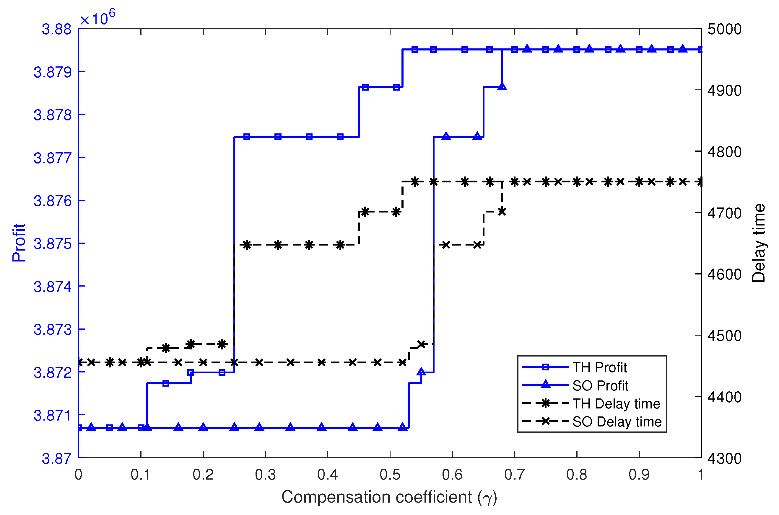
In the following numerical experiments, we set the two objectives having the same relative importance (i.e., $w_1=w_2=0.5$) and tested the solutions of the TH and SO methods with different compensation coefficients $\gamma$. The results of these experiments are reported in

Table 4. Summary of the solutions of the TH and SO methods with different $\gamma$ values.

$\mathit{\gamma }$	TH					SO
	$Z_1$	$Z_2$	${\mu }_1(\%)$	${\mu }_2(\%)$		$Z_1$	$Z_2$	${\mu }_1(\%)$	${\mu }_2(\%)$
0	3,870,698	4456	94.69	100.00		3,870,698	4456	94.69	100.00
0.1	3,870,698	4456	94.69	100.00		3,870,698	4456	94.69	100.00
0.2	3,871,985	4485	94.96	99.65		3,870,698	4456	94.69	100.00
0.3	3,877,474	4647	96.12	97.75		3,870,698	4456	94.69	100.00
0.4	3,877,474	4647	96.12	97.75		3,870,698	4456	94.69	100.00
0.5	3,878,633	4701	96.36	97.12		3,870,698	4456	94.69	100.00
0.6	3,879,512	4750	96.55	96.55		3,877,474	4647	96.12	97.75
0.7	3,879,512	4750	96.55	96.55		3,879,512	4750	96.55	96.55
0.8	3,879,512	4750	96.55	96.55		3,879,512	4750	96.55	96.55
0.9	3,879,512	4750	96.55	96.55		3,879,512	4750	96.55	96.55
1	3,879,512	4750	96.55	96.55		3,879,512	4750	96.55	96.55
Average	3,876,775	4649	95.97	97.73		3,874,519	4580	95.49	98.54

To get more precise solution results, the scales of the satisfaction degrees, ${\mu }_1$ and ${\mu }_2$, in the experiment code are amplified to [0,100].

and illustrated graphically in Figure 2 and Figure 3. As can be observed, several interesting solutions are highlighted in Table 4, which correspond to the conclusion about the same solutions generated by the TH and SO methods given in the previous section. These results totally agreed with the previous theoretical analysis.

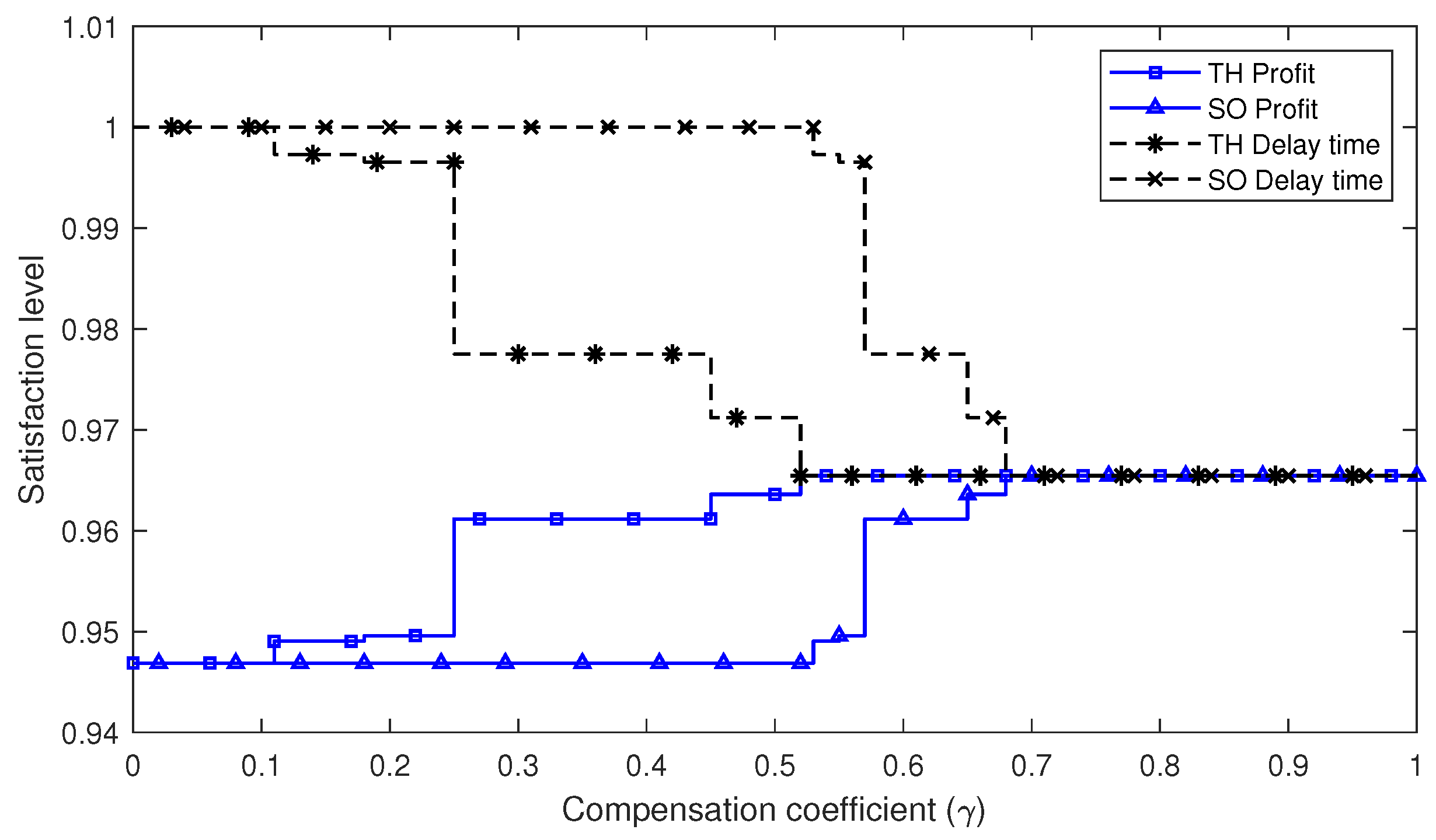
Furthermore, Figure 2 and Figure 3 graphically show the objective function values and the satisfaction levels of the two objectives, respectively. It can be seen that, for both methods, the solutions had a similar changing tendency regarding the variation of the parameter $\gamma$. This was due to the connections between these two methods, which indicated that for each solution of one method, a counterpart could be found in the other method, as discussed in the theoretical analysis. Notably, with the increasing of $\gamma$, both methods tended to get more balanced satisfaction levels of the two objectives.

In total, it could be concluded that the TH and SO methods were both appropriate and qualified methods for solving the proposed MOMILP problem, since they could obtain efficient solutions and all satisfaction degrees of the objectives performed well. However, the TH method is more appropriate when decision makers want to make a clear trade-off between the goals of maximizing the lower bound (i.e., worst case) of the satisfaction degrees or the total (weighted sum) satisfaction degrees of the objectives, as illustrated by Table 1 and Figure 3.

6.3. Impact of Return Rate

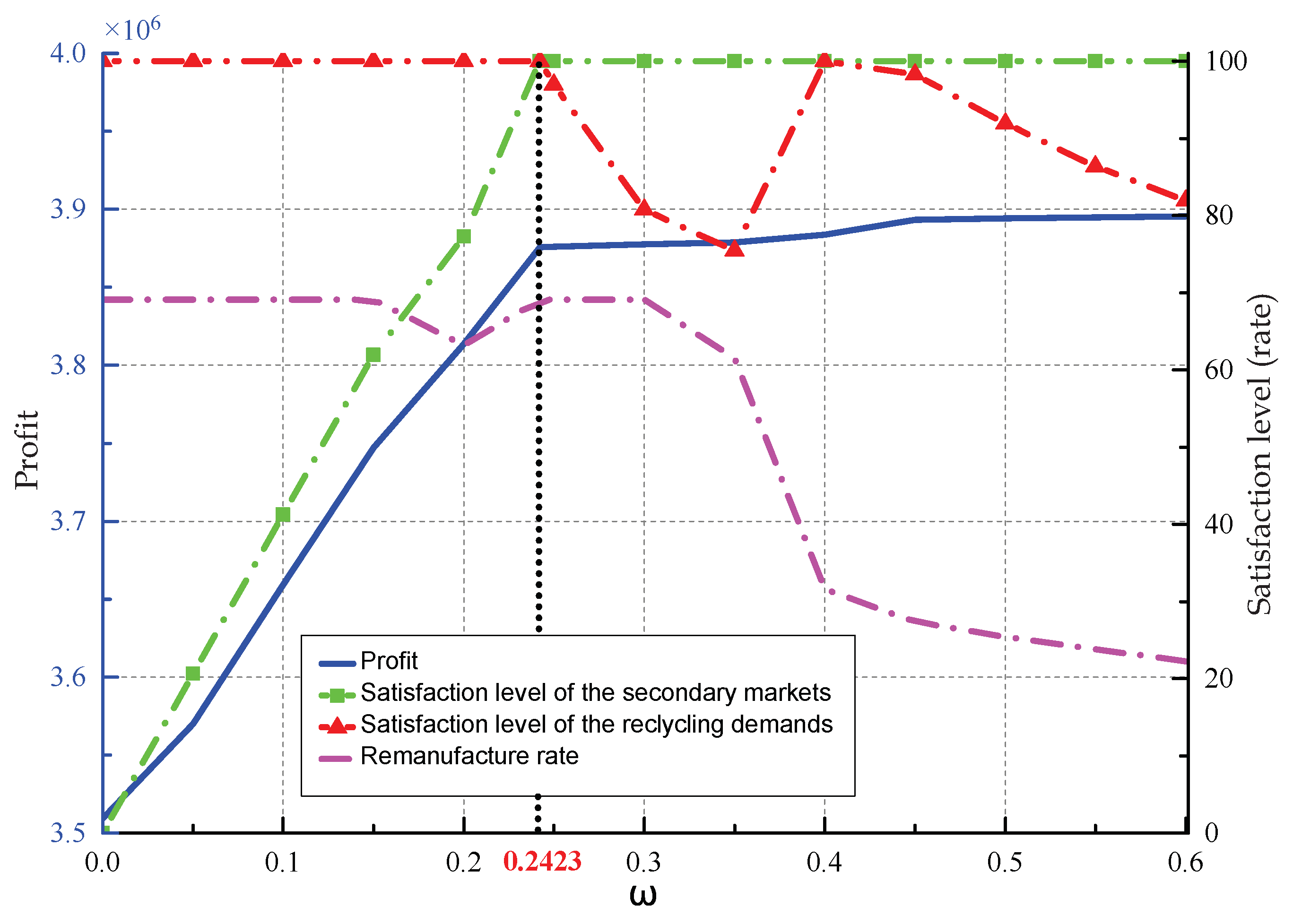
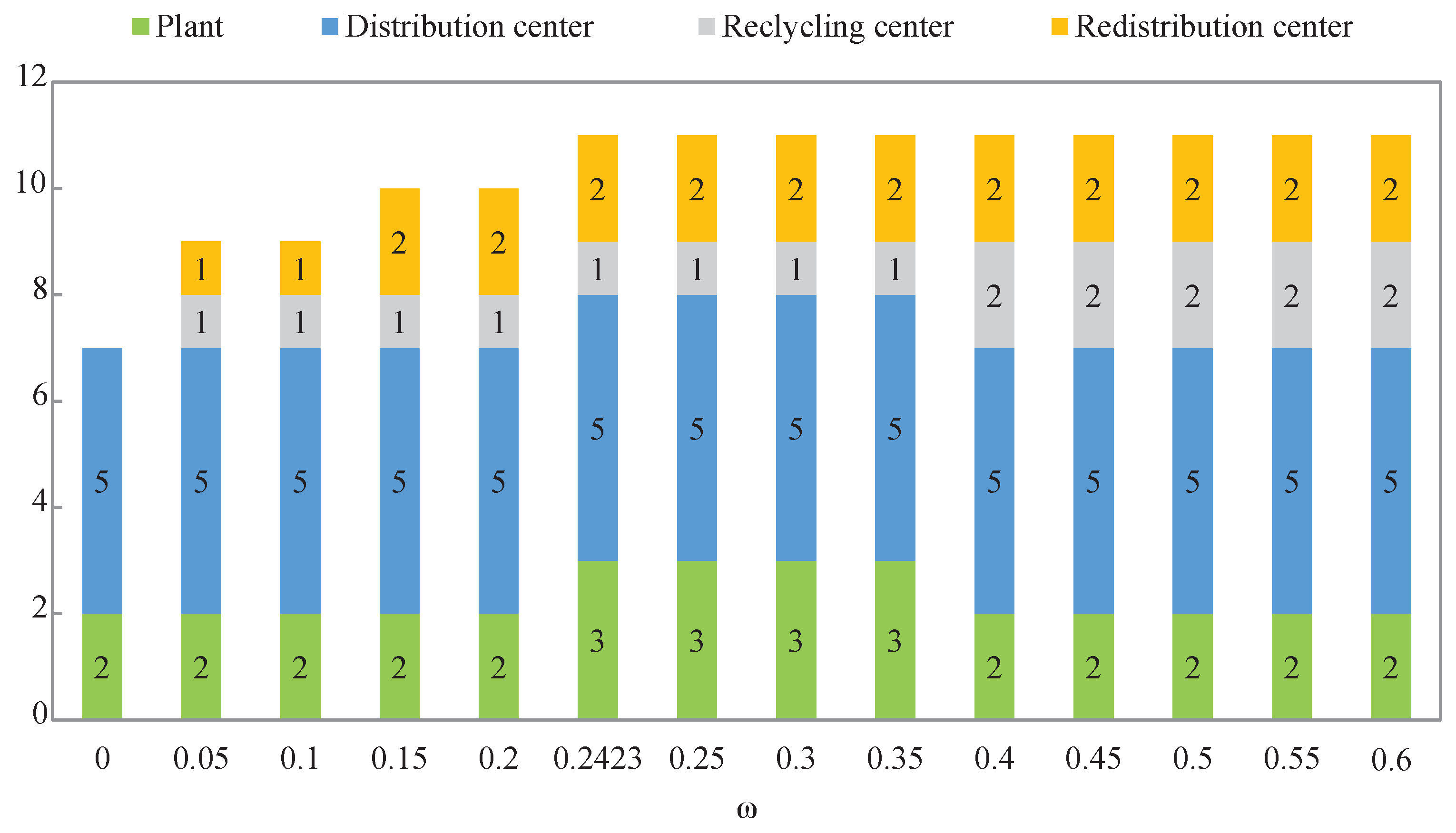
Since the maximum return rate of the used products was an important parameter of the proposed model, we aimed to investigate how the CLSC network structure and profitability changed when the return rate varied. In this regard, test results with a uniform variation of the maximum return rate $\omega$ from 0 to 0.6 (only the profit objective was considered here) are reported in

Table 5. Network structure and profitability with variation of the maximum return rate $\omega$.

$\mathit{\omega }$	Profit	Satisfaction Level of the Secondary Markets	Satisfaction Level of the Recycling Demands	Remanufa -cture Ratio	No. of Plants	No. of Potential Distribution Centers	No. of Potential Collection Centers	No. of Potential Redistribution Centers
0	3,509,219	-	-	-	2	5	0	0
0.05	3,570,049	20.64%	100.00%	69.08%	2	5	1	1
0.1	3,659,171	41.27%	100.00%	69.08%	2	5	1	1
0.15	3,747,184	61.91%	100.00%	69.08%	2	5	1	2
0.2	3,813,807	77.24%	100.00%	63.15%	2	5	1	2
0.2423	3,875,666	100.00%	100.00%	69.08%	3	5	1	2
0.25	3,875,918	100.00%	96.92%	69.08%	3	5	1	2
0.3	3,877,472	100.00%	80.77%	69.08%	3	5	1	2
0.35	3,878,844	100.00%	75.44%	61.48%	3	5	1	2
0.4	3,883,735	100.00%	100.00%	31.58%	2	5	2	2
0.45	3,893,321	100.00%	98.25%	27.34%	2	5	2	2
0.5	3,894,130	100.00%	91.92%	25.42%	2	5	2	2
0.55	3,894,751	100.00%	86.37%	23.83%	2	5	2	2
0.6	3,895,310	100.00%	81.92%	22.25%	2	5	2	2

and Figure 4 and Figure 5.

As shown in Figure 4, it is easy to learn that when the return rate increased, the overall profit increased rapidly at first, but then with a slow growth. To better understand this phenomenon, we further subdivided the parameter $\omega$. It was found that the turning point for the profit growth appeared when the customers’ demands of the secondary markets were just completely satisfied. At this point, $\omega$ equaled 0.2423. The reasons for this could be viewed in two stages: (i) Both the product recycling and remanufacturing could help with increasing the enterprise’s profit. The earnings from the product remanufacturing were greater than the cost of product recycling. Therefore, the reused products flowed into the direction of remanufacturing (also restricted with the capacity of facilities), when the secondary market’s customer demands were not yet satisfied. Hence, the profits grew at a fast speed. (ii) However, when the demands in the secondary markets were all met, the product recycling contributed to the profit’s increasing, but with a slower pace.

Furthermore, whether to recycle products fully according to the maximum return rate depended on the impact on the enterprise profit, as well as the capacities of these facilities (facilities to be opened with different $\omega$ are shown in Figure 5). For further analysis, the satisfaction degree of the recycling demands was defined as the rate of the actual recycling number to the amount generated by the maximum return rate. Figure 4 shows that when $\omega$ was less than 0.2423, the satisfaction level of the recycling-demands was 100%, and when $\omega$ increased from 0.2423 to 0.4, the rate began to drop. However, it regained 100% when $\omega$ was 0.4. Considering the illustration given in Figure 5, the occurrence of this phenomenon was due to the insufficient capacity of the recycling center. Note that the satisfaction degree of the recycling demands showed a downward trend when $\omega$ was higher than 0.4. The overall profit increased with a slow pace, and the number of facilities no longer changed. That also resulted in the immutable capacity of the existing facilities. Hence, the satisfaction level of the recycling demands declined.

In the proposed model, the repairing and disposal rates were fixed. Therefore, from the perspective of profit maximization, the remanufacturing rates should be maintained at the level of 69.08% when $\omega$ was less than 0.2423. However, that was not the case. Figure 4 shows that the minimum value of the remanufacturing rate given $\omega \le 0.2423$ appeared when $\omega =0.2$. Similarly, this was due to the constraint regarding the capacities of the facilities. In addition, Figure 4 also shows that the remanufacturing rates held still after the demands of secondary markets were satisfied. This is because the recycling number was less than the amount generated by the maximum return rate. After that, since all demands of the secondary markets were covered, the remanufacturing rates naturally trended downward with the increase of $\omega$.

From the aforementioned experimental analysis, we could verify the validity of the proposed model in solving the CLSC design problem and the practicability of the solution for offering the enterprise various decision making plans with differing preferences. It is notable that the return rate, as an important parameter in the proposed model, had great impacts on the network structure, as well as the enterprise profits. To this end, the decision maker should pay more attention to the setting of the return rate. With regard to the increase of the return rate, in practice, government incentives and subsidies and growing environmental concern among customers could play a supportive role in product recovery. Besides, from the perspective of enterprise management, setting up an appropriate and flexible CLSC network, as discussed in this study, with specific strategic and tactical plans could also contribute to this goal. In this way, a better implementation of product recovery could be achieved.

7. Conclusions

This paper addressed a closed-loop supply chain network design problem for industrial reuse of products, components, and materials with two objectives, enterprise profit and service level, from the sustainable development perspective. The main conclusions of this paper can be summarized as follows:

(1) A general, but practical network structure supporting multiple recovery options, like repair, remanufacture, redistribution, and recycling, was proposed. Such a configuration catered to the relationship between environment protection and social development. Moreover, market segmentation based on the nature of the products showed the practical significance in the real-life network design.

(2) The $\epsilon$-constraint method and two interactive fuzzy methods (i.e., TH and SO) were adopted to solve the multi-objective network design problem. Furthermore, the proposed multi-objective methods were compared in detail to provide more insights into their relations, which was exactly verified by the numerical experiments. The results also illustrated the viability of both the proposed model and solution approaches.

(3) From the view of the managerial decision, this paper also provided valuable strategic and tactical references on how to promote the economic benefit of the enterprise while achieving sustainable development.

Generally, the proposed model is applicable to any manufacturing industry. Considering the uncertainty about demands, costs, and prices and the complexity in real recycling, production, and transportation scheduling, the future work can be extended to the close-loop supply chain network design for multiple products in multiple periods under an uncertain environment.

References

- Ozceylan, E.; Demirel, N.; Cetinkaya, C. A closed-loop supply chain network design for automotive industry in Turkey. Comput. Ind. Eng. 2017, 113, 727–745. [Google Scholar] [CrossRef]
- Besiou, M.; Georgiadis, P.; Van Wassenhove, L.N. Official recycling and scavengers: Symbiotic or conflicting? Eur. J. Oper. Res. 2012, 235, 563–576. [Google Scholar] [CrossRef]
- Uster, H.; Easwaran, G.; Akcali, E.; Cetinkaya, S. Benders decomposition with alternative multiple cuts for a multi-product closed-loop supply chain network design model. Eur. J. Oper. Res. 2007, 54, 890–907. [Google Scholar]
- Yi, P.; Huang, M.; Guo, L.; Shi, T. Dual recycling channel decision in retailer oriented closed-loop supply chain for construction machinery remanufacturing. J Clean Prod 2016, 137, 1393–1405. [Google Scholar] [CrossRef]
- Devika, K.; Jafarian, A.; Nourbakhsh, V. Designing a sustainable closed-loop supply chain network based on triple bottom line approach: A comparison of metaheuristics hybridization techniques. Eur. J. Oper. Res. 2014, 235, 594–615. [Google Scholar] [CrossRef]
- Giri, B.C.; Sharma, S. Optimizing a closed-loop supply chain with manufacturing defects and quality dependent return rate. J. Manuf. Syst. 2015, 35, 92–111. [Google Scholar] [CrossRef]
- Aras, N.; Aksen, D.; Gonul Tanugur, A. Locating collection centers for incentive-dependent returns under a pick-up policy with capacitated vehicles. Eur. J. Oper. Res. 2008, 183, 1223–1240. [Google Scholar] [CrossRef]
- Maiti, T.; Giri, B.C. Two-way product recovery in a closed-loop supply chain with variable markup under price and quality dependent demand. Int. J. Prod. Econ. 2017, 183, 259–272. [Google Scholar] [CrossRef]
- Wang, F.; Lai, X.F.; Shi, N. A multi-objective optimization for green supply chain network design. Decis. Support Syst. 2011, 51, 262–269. [Google Scholar] [CrossRef]
- Ramezani, M.; Bashiri, M.; Tavakkoli-Moghaddam, R. A new multi-objective stochastic model for a forward/reverse logistic network design with responsiveness and quality level. Appl. Math. Model. 2013, 37, 328–344. [Google Scholar] [CrossRef] [Green Version]
- Verstrepen, S.; Cruijssen, F.; de Brito, M.P.; Dullaert, W. An exploratory analysis of reverse logistics in Flanders. Eur. J. Transp. Infrast. 2007, 7, 142–149. [Google Scholar]
- Fleischmann, M.; Beullens, P.; Bloemhof-Ruwaard, J.M.; Van Wassenhove, L.N. The impact of product recovery on logistics network design. Prod. Oper. Manag. 2001, 10, 156–173. [Google Scholar] [CrossRef]
- Sahyouni, K.; Savaskan, R.C.; Daskin, M.S. A facility location model for bidirectional flows. Transport. Sci. 2007, 41, 484–499. [Google Scholar] [CrossRef]
- Lee, D.H.; Dong, M.; Bian, W. The design of sustainable logistics network under uncertainty. Int. J. Prod. Econ. 2010, 128, 159–166. [Google Scholar] [CrossRef]
- Guide, V.D., Jr.; Danial, R. Prodution planning and control for remanufacturing: industry practice and research needs. J Oper Manag 2000, 18, 467–483. [Google Scholar] [CrossRef]
- Dowlatshahi, S. A strategic framework for the design and implementation of remanufacturing operations in reverse logistics. Int. J. Prod. Res. 2005, 43, 3455–3480. [Google Scholar] [CrossRef]
- Wang, Y.; Chang, X.; Chen, Z.; Zhong, Y.; Fan, T. Impact of subsidy policies on recycling and remanufacturing using system dynamics methodology: a case of auto parts in China. J. Clean. Prod. 2014, 74, 161–171. [Google Scholar] [CrossRef]
- Kannan, G.; Sasikumar, P.; Devika, K. A genetic algorithm approach for solving a closed loop supply chain model: A case study of battery recycling. Appl. Math. Model. 2010, 34, 655–670. [Google Scholar] [CrossRef]
- El-Sayed, M.; Afia, N.; El-Kharbotly, A. A stochastic model for forward-reverse logistics network design under risk. Comput. Ind. Eng. 2010, 58, 423–431. [Google Scholar] [CrossRef]
- Alumur, S.A.; Nickel, S.; Saldanha-Da-Gama, F.; Verter, V. Multi-period reverse logistics network design. Eur. J. Oper. Res. 2012, 220, 67–78. [Google Scholar] [CrossRef]
- Kim, K.; Song, I.; Kim, J.; Jeong, B. Supply planning model for remanufacturing system in reverse logistics environment. Comput. Ind. Eng. 2006, 51, 279–287. [Google Scholar] [CrossRef]
- Dat, L.Q.; Doan, T.T.L.; Chou, S.Y.; Yu, V.F. Optimizing reverse logistic costs for recycling end-of-life electrical and electronic products. Expert. Syst. Appl. 2012, 39, 6380–6387. [Google Scholar] [CrossRef]
- Ramezani, M.; Bashiri, M.; Tavakkoli-Moghaddam, R. A robust design for a closed-loop supply chain network under an uncertain environment. Int. J. Adv. Manuf. Techol. 2013, 66, 825–843. [Google Scholar] [CrossRef]
- Soleimani, H.; Seyyed-Esfahani, M.; Shirazi, M.A. A new multi-criteria scenario-based solution approach for stochastic forward/reverse supply chain network design. Ann. Oper Res. 2016, 242, 399–421. [Google Scholar] [CrossRef]
- Krikke, H.; Bloemhof-Ruwaard, J.; Van Wassenhove, L.N. Concurrent product and closed-loop supply chain design with an application to refrigerators. Int. J. Prod. Res. 2003, 41, 3689–3719. [Google Scholar] [CrossRef]
- Ozkir, V.; Basligil, H. Modelling product-recovery processes in closed-loop supply-chain network design. Int. J. Prod. Res. 2012, 50, 2218–2233. [Google Scholar] [CrossRef]
- Jerbia, R.; Boujelben, M.K.; Sehli, M.A.; Jemain, Z. A stochastic closed-loop supply chain network design problem with multiple recovery options. Comput. Ind. Eng. 2018, 118, 23–32. [Google Scholar] [CrossRef]
- Ozkir, V.; Basligil, H. Multi-objective optimization of closed-loop supply chains in uncertain environment. J. Clean. Prod. 2013, 41, 114–125. [Google Scholar] [CrossRef]
- Talaei, M.; Moghaddam, B.F.; Pishvaee, M.S.; Bozorgi-Amiri, A.; Gholamnejad, S. A robust fuzzy optimization model for carbon-efficient closed-loop supply chain network design problem: a numerical illustration in electronics industry. J. Clean. Prod. 2016, 113, 662–673. [Google Scholar] [CrossRef]
- Soleimani, H.; Govindan, K.; Saghafi, H.; Jafari, H. Fuzzy multi-objective sustainable and green closed-loop supply chain network design. Comput. Ind. Eng. 2017, 109, 191–203. [Google Scholar] [CrossRef]
- Masoudipour, E.; Amirian, H.; Sahraeian, R. A novel closed-loop supply chain based on the quality of returned products. J. Clean. Prod. 2017, 151, 344–355. [Google Scholar] [CrossRef]
- Selim, H.; Ozkarahan, I. A supply chain distribution network design model: An interactive fuzzy goal programming-based solution approach. Int. J. Adv. Manuf. Techol. 2008, 36, 401–418. [Google Scholar] [CrossRef]
- Pishvaee, M.S.; Torabi, S.A. A possibilistic programming approach for closed-loop supply chain network design under uncertainty. Fuzzy. Set. Syst. 2010, 161, 2668–2683. [Google Scholar] [CrossRef]
- Khajavi, L.T.; Seyed-Hosseini, S.M.; Makui, A. An integrated forward/reverse logistics network optimization model for multi-stage capacitated supply chain. iBusiness 2011, 3, 229. [Google Scholar] [CrossRef] [Green Version]
- Zarbakhshnia, N.; Soleimani, H.; Goh, M.; Razavi, S.S. A novel multi-objective model for green forward and reverse logistics network design. J. Clean. Prod. 2019, 208, 1304–1316. [Google Scholar] [CrossRef]
- Haimes, Y.Y.; Lasdon, L.S.; Wismer, D.A. On a bi-criterion formation of the problems of integrated system identification and system optimization. IEEE Trans. Syst. Man. Cybernet. 1971, 3, 296–297. [Google Scholar]
- Zimmermann, H.J. Fuzzy programming and linear programming with several objective functions. Fuzzy Set. Syst. 1978, 1, 45–55. [Google Scholar] [CrossRef]
- Li, X.; Zhang, B.; Li, H. Computing efficient solutions to fuzzy multiple objective linear programming problems. Fuzzy Set. Syst. 2006, 157, 1328–1332. [Google Scholar] [CrossRef]
- Werners, B. An interactive fuzzy programming system. Fuzzy Set. Syst. 1987, 23, 131–147. [Google Scholar] [CrossRef]
- Torabi, S.A.; Hassini, E. An interactive possibilistic programming approach for multiple objective supply chain master planning. Fuzzy Set. Syst. 2008, 159, 193–214. [Google Scholar] [CrossRef]
- Farrokh, M.; Azar, A.; Jandaghi, G.; Ahmadi, E. A novel robust fuzzy stochastic programming for closed loop supply chain network design under hybrid uncertainty. Fuzzy Set Syst 2017, 341, 69–91. [Google Scholar] [CrossRef]
Figure 1.
The closed-loop supply chain (CLSC) network with multiple recovery options.
Figure 2.
Objective function values of the TH and SO methods with different values.
Figure 3.
Objective satisfaction levels of the TH and SO methods with different values.
Figure 4.
Effect of on enterprise profit and flow distribution.
Figure 5.
Effect of on the number of facilities.