Neighborhood Walkability and Housing Prices: A Correlation Study


1
Department of Urban Planning, Keimyung University, Daegu 42601, Korea
2
Department of Civil and Environmental Engineering, Seoul National University, Seoul 08826, Korea
*
Author to whom correspondence should be addressed.
Sustainability 2020, 12(2), 593; https://doi.org/10.3390/su12020593
Submission received: 17 December 2019
/
Revised: 8 January 2020
/
Accepted: 10 January 2020
/
Published: 13 January 2020
(This article belongs to the Special Issue Walkable living environments)
Abstract
:This study aims to examine the relationship between the level of walkability and housing prices in Seoul, Korea. The average transaction price per square meter for each apartment complex was set as a dependent variable and the walkability score was used as an independent variable. This study divided a total of 5986 apartment complexes into areas with high and low housing prices for analysis. Based on the strong spatial autocorrelations of housing prices, this study employed spatial regression models in addition to the Ordinary Least Squares (OLS) model. Results showed that housing prices positively correlated with the walkability score in areas with low housing prices, whereas no significant association was observed in areas with high housing prices. Additional findings showed that housing prices were associated with building age (−), number of households in the complex (+), slope (−), and greenness (+) in both subsamples. Results also showed that high school quality had a different association with housing prices depending on the subsample (e.g., the sign was positive in areas with high housing prices and no significance in areas with low housing prices). The results herein support public policy proposals relevant to urban planning, environmental design, and housing policies.
1. Introduction
Walkable environments correlate with increased walking, biking, and physical activity [1,2,3], a reduction in diseases, and an improvement in overall health [4,5,6,7]. Moreover, increasing evidence has suggested that a walkable environment can have an impact on environmental and social benefits. A walkable environment may improve air pollution through reduced use of vehicles [8,9,10], increased safety through reduced crime rates [11,12,13], and promote social cohesion through increased social interaction among residents [14,15]. Therefore, many professionals, including urban planners and designers, transportation engineers, environmental scientists, public health scientists, and even policy makers, endeavor to create walkable environmental conditions in urban contexts.
In 2016, the city of Seoul implemented a project called “Walkable City, Seoul” to improve Seoul’s pedestrian environment and its citizens’ quality of life. To launch this project, the city of Seoul suggested the slogan, “Good bye Car, Good day Seoul” and implemented four policy directions, including “Possible to walk”, “Easy to walk”, “Want to walk”, and “Walk together” [16]. Before “Walkable City, Seoul” was launched, Seoul had made significant efforts to create a pedestrian-friendly environment, and perhaps as a result of that, the health behavior of Seoul citizens has increased over the past decade. According to the Community Health Survey, the rate of walking has increased from 57.3% (2008) to 61.5% (2017), while the rate of moderate to vigorous physical activity has also increased from 19.1% (2009) to 22.2% (2017) over the last decade [17].
As mentioned above, a walkable environment has many health, environmental, and social benefits, so it may also be considered one of the most important factors in residents’ choice of housing, and it may even affect housing prices. Many empirical studies show that the level of walkability in a neighborhood has a positive correlation with property values [18,19,20,21,22]. For example, Leinberger and Alfonzo found that the housing prices in walkable neighborhoods were higher than those in less walkable neighborhoods in Washington, D.C. [18]. Some researchers have employed the walk score as an indicator of the walkability level and have used it to estimate the impact on real estate values. Cortright conducted a study in 15 metropolitan areas in the United States and found that when the walk score increased by an additional one point, housing prices would increase from US $700 to $3000 [19]. Washington focused on 259 large cities with a population of over 100,000 in the United States and found that a one-point increase in the walk score would increase housing prices by about 0.5% [20]. Pivo and Fisher found that a 10-point increase in the walk score value increased the property value by 1% to 9%, depending on the type of property in the United States [21]. Rauterkus and Miller also found a significantly positive relationship between the walk score and land values in Jefferson County, Alabama [22]. These studies were all carried out in the United States because walk score data by address are only available in the United States and Canada [23].
This has led to many efforts to develop the walkability indicator adapted from the walk score methodology in Europe and Asia. Reyer et al. tried to develop the walk score and investigate its association with active transportation in Stuttgart, Germany [24]. Zhang et al. also calculated the walkability level and defined its relationship with residential estate value in Futian District, China [25]. In particular, Zhang and colleagues’ study found a negative association between walkability and housing prices in 2018. In Korea, efforts have been made to produce walkability data, and Kim et al. calculated the walkability score throughout all of Seoul. As in the case of Stuttgart and Futian, Seoul’s walkability score was basically adopted from the walk score methodology derived from the United States [26].
How does the walkability score correlate with housing prices in Seoul? It may be negatively correlated, as was the case in Zhang and colleagues’ study, or positively correlated, as in other studies carried out in the United States. As shown in previous studies in the United States, the level of walkability is calculated based on the accessibility of the amenities local residents need to live their daily lives, which is typically reflected in the neighborhood’s housing prices [18,19,20,21,22]. On the other hand, Zhang and colleagues’ study obtained a contrary result, because their study area (Futian District, China) was characterized by rapid urbanization and car-dependent urban form. Therefore, it can be inferred that housing prices in Futian District may have been more influenced by factors other than the walkability of the neighborhood. There has been little research on the relationship between walkability and housing prices using objectively measured variables in Seoul, Korea. The aim of this study is to examine the relationships between the level of environmental walkability and housing prices at the neighborhood level. The walkability score is identified as the key independent variable in this research. The following hypothesis will be tested:
H1.
Areas with more walkable environments have a higher housing price than those with less walkable environments.
2. Materials and Methods
2.1. Study Area
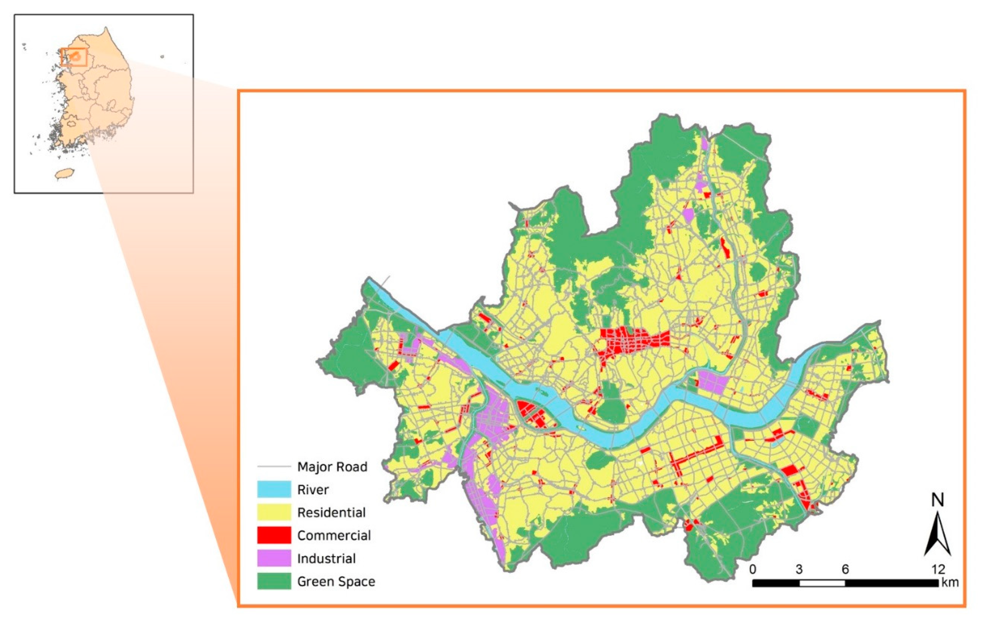
The city of Seoul, Korea was the area of study, as shown in Figure 1. Seoul is the capital of Korea and is located in the northwest portion of the country. Over 50% of its area is residential, while commercial and industrial areas cover 4.18% and 3.30%, respectively. Almost 40% is green space, much of which was designated as greenbelts and rivers as of 2017 [27]. Housing policy is one of the major policy issues for Seoul. The total area of Seoul is approximately 605 km2 which constitutes 0.60% of the whole country; meanwhile, the total population is 9,857,426, which was almost 19.04% of the national population as of 2017 [28]. As shown by these statistics, Seoul’s population density is very high; thus, housing demand has increased, and housing prices have risen steadily and rapidly [29]. Therefore, finding a solution to this problem has always been an important task, not only for the Seoul Metropolitan Government but also at the national level [30]. Further, apartments have consistently been the dominant housing type in Seoul, Korea, and the government sector is expected to maintain and manage apartment complexes as a key focus of its residential policy [31,32].
2.2. Variables: Data
2.2.1. Housing Price: Dependent Variable
Because of their predominance and importance, apartments have been used as a representative variable for Korean housing and residential research in many previous studies [31,32,33,34]. This study examines all apartment complexes traded in Seoul, 2017. There were 106,292 housing transactions in 5986 apartment complexes. The spatial unit of analysis of the study was the individual apartment complex, and the average transaction price per square meter for each of the 5986 apartment complexes was used as a dependent variable. The data were provided for research purposes from the Korea Appraisal Board (http://www.kab.co.kr/kab/home/eng/main.jsp) [35].
2.2.2. Walkability Score: Key Independent Variable
This study employs the walkability score as an independent variable. The walk score is an index that measures the level of walkability using nine types of access to destinations and two variables for pedestrian friendliness, as shown in Table 1. The number in the “Count” column indicates the number of amenities included in the walk score calculation. When calculating the walk score at a particular location, the grocery store only included the nearest one, while the shopping center included up to the nearest five. The grocery store weighted three points to the nearest one, while the shopping center weighted five facilities to 0.5, 0.45, 0.4, 0.35, and 0.3 respectively, depending on the distance. Meanwhile, intersection density and average block length were considered as measures of pedestrian friendliness, and areas with poor pedestrian friendliness were penalized up to 10% [36]. Because the walk score is one of the most popular indices, many studies have used it as an index of walkability level in the environment [37,38,39,40,41,42].
Walk score data are available for a few countries, such as the United States and Canada, but are not available in Korea. Therefore, Kim et al. used the walk score methodology to produce a walkability score in Seoul. The walkability score data for Seoul that were used in this study came from their research; more detailed information about the data and methods can be found in [26].
2.2.3. Apartment Complex Characteristics and Neighborhood Environmental Variables: Confounding Variables
The confounding variable comprised characteristics of the apartment complex and neighborhood environmental conditions. The characteristics of the apartment complex were the built environmental conditions within a given complex, whereas those of the neighborhood were the environmental characteristics outside of the complex.
• Building Age and the Number of Households
The characteristics of the apartment complex included building age and the number of households in the complex. The data for building age and the number of households in the apartment complex were acquired from the internal data of the Korea Appraisal Board.
• Quality of High School
The neighborhood environmental conditions included the quality of high schools, access to the subway station, slope, and greenness. The quality of schools is one of the most important factors in housing prices, as described in previous studies [43,44,45,46]. Some studies found that school performance had a greater impact on housing prices in Korea [47,48,49]. One of these studies, Bae and Chung [48], found that school quality was significantly correlated with housing prices in the Seoul Metropolitan Area. As a measure of school quality, they used the number of students per 1000 graduates entering Seoul National University, which is considered the most prestigious university in Korea [48]. In Seoul, students were allocated to local high schools based on their residence; therefore, the location of high schools with high admission rates to prestigious universities can be a very important neighborhood environment factor for parents. The SKY is an abbreviation formed from the first letters of three prestigious universities in Korea: Seoul National University, Korea University, and Yonsei University. This study included the SKY league admission rate as a confounding factor to indicate high school quality in a given neighborhood. The variable is defined as the SKY league admission rate of the nearest high school within a 4 km airline buffer from the centroid of an apartment complex.
The walkability score is an index based on access to nine types of destination facilities needed in daily life. Since elements such as access to subway stations, slope, and greenness were not included as environmental factors affecting the level of walkability in the walkability score calculation method, these three variables were also added into this study for use in the analysis.
• Access to Subway Stations
This study includes the variable of access to subway stations for the analysis. Access to subway stations is a significant factor in land prices [50,51,52]. In Korea, a concept of “access to subway stations” has been used as the name of the “station catchment area” [53], and several studies have been conducted on how access to subway stations affects local land prices [54,55]. As a variable of access to subway stations, the network distance from the centroid of an apartment complex to the nearest subway station is captured through Geographic Information System (GIS).
• Slope
Many studies have revealed a correlation between slope and the level of walkability [56,57]. In particular, the slope was more sensitive to the walking behavior for the elderly [58,59,60]. In this study, the slope is included as an environmental variable and is defined as the mean slope within a 400 m network buffer from the centroid of an apartment complex.
• Greenness
This study includes the level of greenness measured by the (normalized difference vegetation index (NVDI) as a variable to measure the neighborhood’s environmental quality. Although the walkability score includes access to parks, it is considered that the greenness factor should be examined further because of its impact on the walkability of the neighborhood environment [61,62,63]. NDVI is the most common index quantifying vegetation using remote sensing [64,65,66,67]. The range of NDVI values is from −1 (no vegetation) to 1 (green vegetation). The higher the NDVI value, the greener and healthier the vegetation conditions [66,67]. For this study, the Landsat-8 OLI scene of 6 May 2017 (path 116/row 34), throughout the Seoul area, was obtained from the United States Geological Survey (USGS) website (https://earthexplorer.usgs.gov/) [68]. To extract the NDVI values, the following Equation (1) was used [69,70]. In the case of Lansat-8 OLI, near-infrared (NIRED) refers to band 5 and infra-red (RED) refers to band 4 [71]. The variable is defined as the mean NDVI within a 400 m network buffer from the centroid of an apartment complex.
2.2.4. Variables and Their Measurements and Data Sources for Modeling
The variables used to verify the research hypothesis in the model are organized as shown in Table 2. Housing price was an independent variable, whereas the walkability score was a dependent variable. The confounding variables comprised the built environmental factors and were classified into characteristics of a complex (inside an apartment complex) and neighborhood environment (outside of an apartment complex). The characteristics of a complex variable were the building age and the number of households. The variable regarding the neighborhood environment included the quality of the high school, access to subway stations, slope, and greenness. This study used data collected in 2017 to analyze all variables, except for that of high school quality. Because the level of high school quality is not provided to the public on an annual basis, no data were found on this variable from 2017, and this study therefore utilized data collected in 2012.
2.3. Statistical Analysis
To capture the environmental variables, ArcGIS 10.6 (Esri, Redlands, California, United States) was used. The spatial regression model and the Ordinary Least Squares (OLS) regression were implemented to examine the relationship between the walkability score and housing prices using GeoDa 1.14.
3. Results
3.1. Descriptive Statistics and Bivariate Analysis of Walkability Score and Housing Price
3.1.1. Overall Descriptive Statistics and Spatial Patterns
Table 3 shows the descriptive statistics of the walkability score and the housing prices of 5986 apartment complexes. Based on the dataset in Seoul (N = 44,000), the walkability score value closest to the apartment complex was taken as its walkability score at the corresponding apartment complex. The average walkability score of 5986 apartment complexes was 72.59 (SD = 8.06), with a maximum value of 94.67. Meanwhile, the average housing price of the 5986 apartment complexes was 6.10 million won/m2 (approximately US $5545/m2), with a maximum value of 25.94 million won/m2 (approximately US $23,582/m2), indicating a very large deviation.
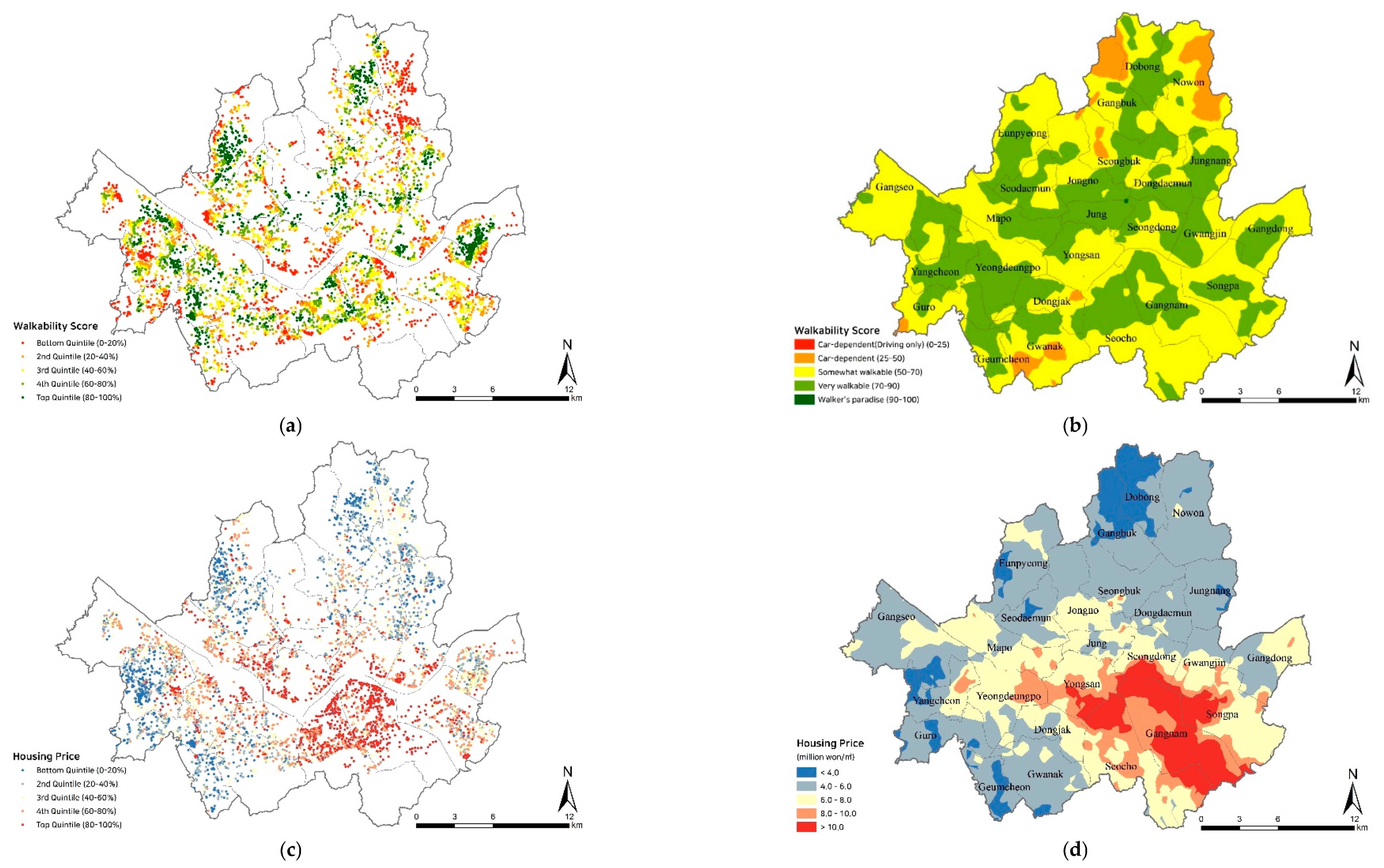
Figure 2a shows the quintile map of the walkability score for 5989 apartment complexes, while Figure 2b is a walkability score map that was generated and interpolated from Figure 2a using the ordinary kriging method. The average walkability score per apartment complex appeared to be distributed across Seoul without any particular clustering. Meanwhile, Figure 2c shows the quintile map of the housing prices for 5986 apartment complexes, and Figure 2d is the interpolated map comprising the housing price from Figure 2c. As shown in these two figures (Figure 2c,d), the average housing price per apartment complex in Seoul was generally very high in the southeastern regions of Seocho-gu, Gangnam-gu, and Songpa-gu, as well as Yongsan-gu and Seondong-gu, which are located in the central region. In contrast, the areas with low housing prices were clustered in northern and southwestern Seoul.
As shown in Figure 2, the walkability score did not have a regional cluster, while the housing price had a very distinct regional clustering pattern. Housing price was very high in the southeastern part of Seoul. Many studies have shown that the housing price and level of walkability have a positive correlation [19,20,22]. Meanwhile, a study by Zhang et al. showed that the housing price was negatively correlated with the level of walkability in the Futian district in Shenzhen, China [25]. Our task here was to analyze these aspects as they relate to Seoul, Korea.
As shown in Table 4 below, there was no significant correlation between the housing price and the walkability score when including all 5986 apartment complexes. However, as seen in Figure 2, the walkability score did not reveal a clear clustered pattern, but the housing price was very high in the southeastern part of the city. Therefore, it was necessary to divide the sample of 5986 apartment complexes into subareas comprising high and low housing prices, respectively.
3.1.2. Descriptive Statistics and Spatial Patterns by Subsample
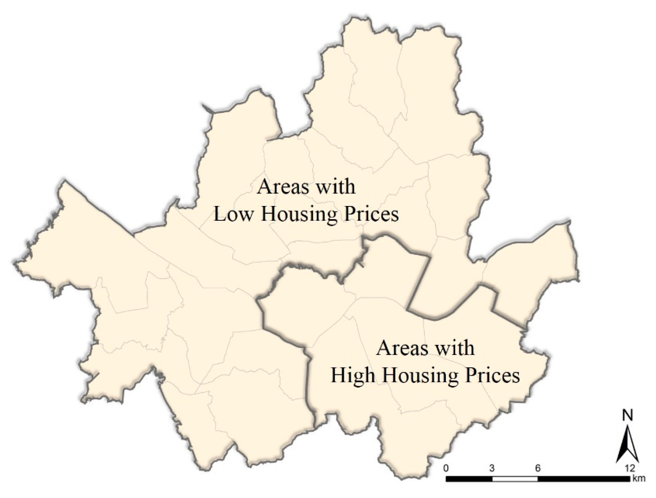
As seen in Figure 2c,d above, we decided to classify the southeastern part of the city, wherein housing prices were distinctly high, as areas with high housing prices and established the rest as areas with low housing prices. Areas with high housing prices were Gangnam-gu, Seocho-gu, Songpa-gu, Yongsan-gu, and Seongdong-gu, in which the average housing prices were in the city’s top 30%. Figure 3 describes a classification of subsamples divided as follows: “Areas with high housing prices” and “Areas with low housing prices”.
When we analyzed the areas with high and low housing prices separately, the correlations between housing prices and the walkability score contrasted. In areas where housing prices were high, housing prices and the walkability score were not significantly correlated. However, in areas where housing prices were low, a positive correlation between them was revealed, as shown in Table 4 (Pearson correlation coefficient = 0.076, p < 0.001).
As explained in Section 2.2, the variables used for modeling are shown in Table 5. Some variables, including housing price, number of households, distance to subway station, mean slope, and mean NDVI, were transformed into logged values to analyze the regression model. Table 5 also provides descriptive statistics of variables across low and high housing price subsamples.
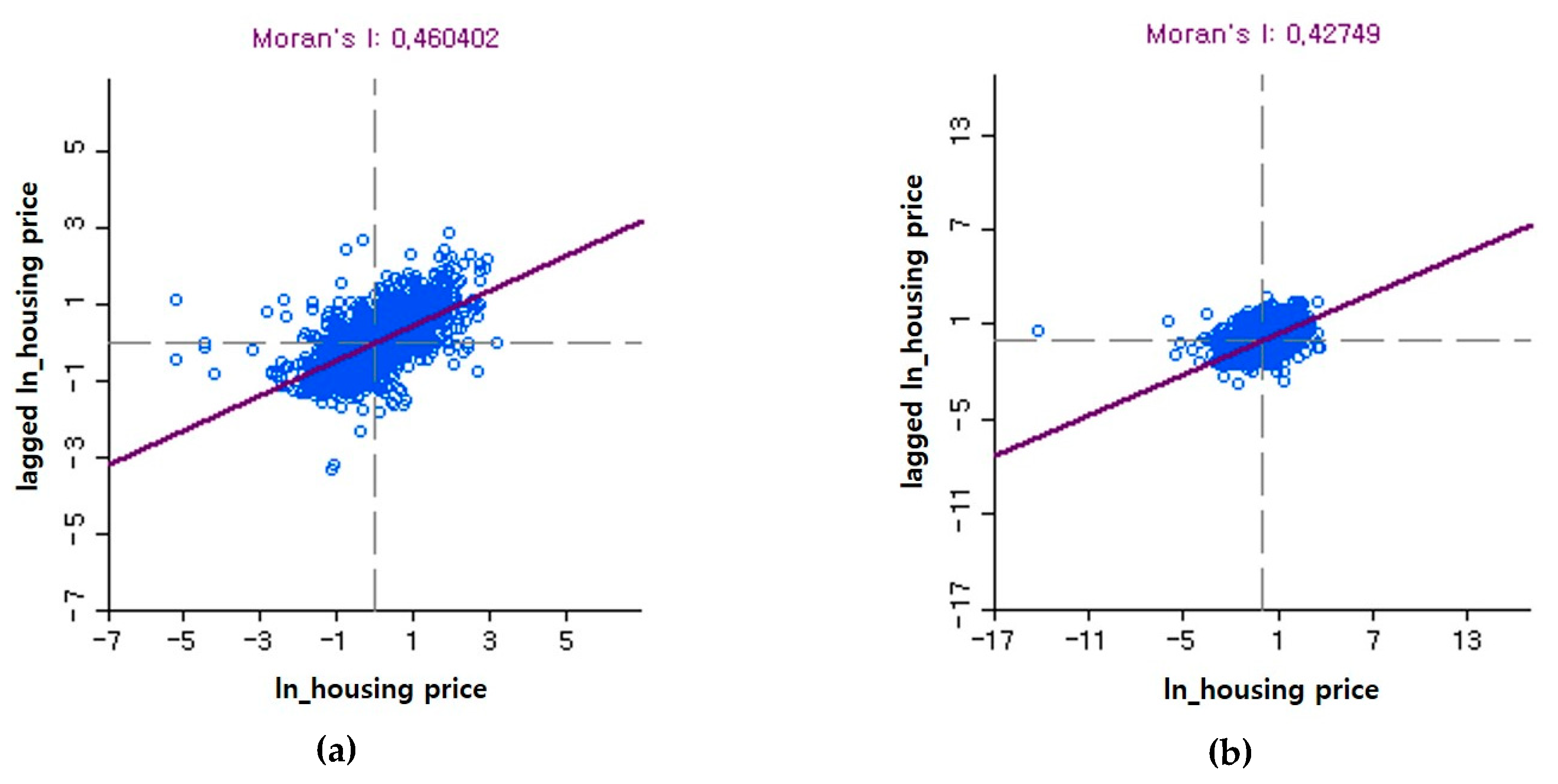
As shown in Figure 4, the univariate Moran’s I of housing prices in areas with high and low housing prices using the 400 m distance spatial weights were 0.460 and 0.427, respectively. Both the Moran scatter plots described strong slopes, and most respondents converged on the fitted lines. The plots showed that housing prices in both areas had strong, positive autocorrelations.
3.2. Multivariate Analysis
Because of the evidence of strong spatial autocorrelations of housing prices in both subsamples, an OLS regression model was insufficient to explain the correlates between housing prices and the walkability score. Therefore, this study employed spatial regression models in addition to the OLS model, as shown in Table 6.
3.2.1. Subsample: Areas with High Housing Prices
According to the Breusch–Pagan and several other spatial dependence tests, there was strong heteroscedasticity and spatial dependence. A Moran’s I score of 0.460 indicated evidence for a strong spatial autocorrelation at the 0.01 significance level. Therefore, it became necessary to introduce a spatial regression model. This study employed two types of spatial regression models including the spatial lag model (SLM) and the spatial error model (SEM). The spatial dependence of the SLM was captured by spatial spillover effects and spatial error correlation effects, while the spatial dependency of the SEM was captured only by spatial error correlation [75,76]. The introduction of the spatial regression model improved the general model fit, as indicated in the higher values of the R-square and the log-likelihood. The R-squares of the OLS, the SLM, and the SEM were 0.407, 0.487, and 0.609, respectively, while the log-likelihood of the model developed from −215.224 (OLS) to −113.004 (SLM), and further to 36.435 (SEM). The P-values from the Breusch–Pagan and likelihood ratio tests (of the SLM and the SEM, respectively) were less than 0.001. Further, the highly significant parameters of rho (ρ) and lambda (λ) indicated significant spatial dependencies. The SEM would be the best model for use in this case based on the model performance parameters (e.g., R-square and log-likelihood).
The findings of housing prices following SEM analysis are as follows. First, housing prices did not have any significant association with the walkability score. This finding did not support the hypothesis that the areas with more walkable environments have a higher housing price than that of areas with less walkable environments. This implies the existence of very important variables that affect housing prices other than the level of neighborhood walkability. Second, the housing price was correlated with building age (−) and the number of households (+). This means that the more recent the construction and the higher the number of households in an apartment complex, the higher the housing price. Third, housing price had a negative relationship with the mean slope, while it was positively related to mean NDVI. This finding may support the hypothesis that areas with more walkable environments promoting walking and physical activity have a higher housing price. Meanwhile, the distance to subway stations had no significant relationship with housing prices. Fourth, the SKY league admission rate, which was used as a measure of high school quality, had a significantly positive correlation with housing price. This was the same result as that obtained in many previous studies [43,44,45,46,47,48,49].
3.2.2. Subsample: Areas with Low Housing Prices
A Moran’s I score of 0.427 indicated evidence for a strong spatial autocorrelation at the 0.01 significance level. These limitations necessitated the introduction of a spatial regression model rather than an OLS regression model. The R-square increased from 0.412 to 0.623, and the log-likelihood also improved from −95.046 to 661.968. However, spatial dependencies still existed according to the likelihood ratio test. Moreover, the spatial autoregressive coefficients in the SLM (e.g., ρ = 0.315, p-value < 0.001) and the SEM (e.g., λ = 0.677, p-value < 0.001) were highly significant. Similar to the model with high housing price areas, the SEM would be the best model to use based on the model performance parameters.
The results of this analysis are summarized as follows. First, housing price was positively correlated with the walkability score after controlling for confounding variables. This finding supported the hypothesis that areas with more walkable environments have a higher housing price than those with less walkable environments. Second, the housing price was negatively correlated with building age, while it was positively related to the number of households in an apartment complex. This aligns with previous findings derived from a model using a subsample of areas with high housing prices. Third, housing price was correlated with distance to subway station (−), mean slope (−), and mean NDVI (+). All three variables were related to neighborhood environments and promote walking and physical activity. Some studies reveal that easy access to subway stations, fewer slopes, and more greenness in the environment tended to encourage walking and, therefore, promoted physical activity [56,77,78,79,80,81]. Finally, results showed that as a measure of high school quality, the SKY league admission rate had no significant correlation with housing price. This is a different result from a previous study of areas with high housing prices.
3.2.3. Summary
In summary, the level of walkability and the built environmental correlated with housing price are synthetically summarized again as follows. The overall findings supported the hypothesis, which asserted that areas with more walkable environments have a higher housing price than those with less walkable environments. Based on the spatial regression model, the variable indicating the walkable environmental conditions includes easy access to subway stations, fewer slopes, and the increased greenness of neighborhood environments. However, some results differed between the two subsamples: the housing price positively correlated with the walkability score in areas with low housing prices, whereas no significant association was observed in areas with high housing prices. The overall findings show that the role of the built environment may be important in determining housing prices. Another interesting finding is that SKY league admission rates had different effects on housing prices depending on the subsample. A positive correlation was revealed between SKY league admission rates and housing prices in areas with high housing prices, while no significant relationship was observed between them in areas with low housing prices.
4. Discussion and Conclusions
It is often said that a walkable environment is one of the most important factors in selecting a residence. People want to walk and ride bikes in their neighborhoods. Some studies show that the level of walkability in neighborhoods is positively correlated with housing prices [18,19,20,21,22]. The walk score is widely used as an indicator of the walkability level in a neighborhood [82]. This study examined 5986 apartment complexes in Seoul, Korea, all of which had conducted transactions in 2017. Using both spatial regression models and the OLS regression model, we established and empirically analyzed our research hypothesis as follows: “Areas with more walkable environments have a higher housing price than those with less walkable environments”.
The overall findings of the study are summarized in the following points. First, the hypothesis of this study is half correct. There was no significant relationship between the walkability score and housing prices across all of Seoul, but different results were revealed when Seoul was divided into two subsamples: a significant correlation was revealed between the walkability score and housing prices in areas with high housing prices, whereas no statistical relationship existed between them in areas with low housing prices. When considering the level of walkability as a factor influencing housing prices, it is difficult to encapsulate the entire housing market in Seoul. Second, although the relationship was only statistically significant in areas with low housing prices, a positive correlation was observed between the walkability score and housing prices, as shown in previous studies in the United States [19,20,21,22]. In particular, results showed that a one-point increase in the walkability score would increase housing prices by about 0.2% in areas with low housing prices. Third, there was no significant correlation between the walkability score and housing prices in areas with high housing prices. Interestingly, the quality of high school, as measured by the SKY league admission rate, was a very important factor for housing prices in areas with high housing prices. In Seoul, schools of good quality are mostly located in areas with high housing prices [47,48], consequently, the result showed a strong, positive correlation with the quality of high school and housing prices in those areas. This is in line with the results of preceding studies, which showed that the quality of the high school in the Gangnam Area (commonly referenced as Gangnam-gu, Seocho-gu, and Songpa-gu) is a very important factor in the elevation of housing prices [47,48,49]. In addition, this can be interpreted as representing the symbolic characteristics of the Gangnam Area in Seoul. The Gangnam Area transcends its function as simply a residential area, as the residents who live there also assume a socially superior status. That is, the level of walkability in the neighborhood may not be considered in the Gangnam Area and its neighboring districts as a factor in determining housing prices. Fourth, additional environmental variables were correlated with housing prices. The distance to the subway station had a significantly negative correlation with housing prices in areas with low housing prices, while no statistical relationship was found between them in areas with high housing prices. This result could be explained with the relatively high dependence on public transport in areas with low housing prices compared to that of areas with high housing prices. Housing prices were significantly associated with the mean slope (−) and the mean NDVI (+) of neighborhood environmental conditions in both subsample areas.
Although this study provides a greater understanding of the relationship between walkability and housing prices in Seoul, it has several limitations, which suggest directions for future studies. First, the walkability score needs to be revised and developed to better evaluate the level of walkability in a given neighborhood. Although the factor of park accessibility was already considered in the walkability score calculation, the mean NDVI showed a positive correlation with housing prices. This means that greenness can be an important factor that cannot be overemphasized in residential housing selection for urban dwellers. When developing the walkability index in further study, it is necessary to give greater consideration to the greenness factor. Second, it is required to divide Seoul into more disaggregated areas to examine the correlation between the level of walkability and housing prices. Based on the examination of the spatial patterns of the walkability score and the housing prices, this study divided Seoul into two groups (the top 30% of the housing prices vs. the bottom 70% of the housing prices). To produce more meaningful results, future research may allow further subdivision of groups (e.g., subdivisions by 25 municipalities). This can help to suggest practical implications for establishing housing and/or urban regeneration policies. Moreover, another limitation of this study is its cross-sectional design. It is necessary to examine the correlation between the walkability and housing prices in areas where housing prices have recently surged and/or markedly dropped. If we examine the correlation between these two factors before and after the housing price transition, this would give us a closer look at the importance of walkability level as a determinant of housing prices.
This study examined the correlation between the level of walkability and housing prices, which has been studied substantially in the United States and other countries. It is meaningful to analyze 5,986 apartment complexes throughout all of Seoul, not limited to some districts. Following our examination of the hypothesis regarding the correlation between walkability and housing prices, we also observed an additional interesting result: the correlation differed depending on a given area. This study is significant because it revealed a positive correlation between walkability and the housing prices in areas with low housing prices; meanwhile, no significant relationship was observed in areas with high housing prices. This suggests that policies tailored to regional characteristics need to be addressed. The results of this study can be used to suggest public policy proposals in urban planning, environmental design, and housing policies.
Author Contributions
Conceptualization, E.J.K. and H.K.; Methodology, E.J.K. and H.K.; Software, E.J.K.; Validation, E.J.K. and H.K.; Formal Analysis, E.J.K.; Investigation, E.J.K.; Resources, E.J.K.; Data Curation, E.J.K.; Writing—Original Draft Preparation, E.J.K. and H.K.; Writing—Review and Editing, E.J.K. and H.K.; Visualization, E.J.K.; Supervision, E.J.K.; Project Administration, E.J.K.; Funding Acquisition, E.J.K. All authors have read and agreed to the published version of the manuscript.
Funding
This work was supported by the National Research Foundation of Korea (NRF) grant funded by the Korean government (MSIT) (No. NRF-2017R1A2B4005440).
Conflicts of Interest
The authors declare no conflicts of interest. The funders had no role in the design of the study; in the collection, analyses, or interpretation of data; in the writing of the manuscript, or in the decision to publish the results.
References
- Brown, B.B.; Smith, K.R.; Hanson, H.; Fan, J.X.; Kowaleski-Jones, L.; Zick, C.D. Neighborhood design for walking and biking. Am. J. Prev. Med. 2013, 44, 231–238. [Google Scholar] [CrossRef] [Green Version]
- Saelens, B.E.; Handy, S.L. Built environment correlates of walking. Med. Sci. Sports Exerc. 2008, 40, S550–S566. [Google Scholar] [CrossRef] [Green Version]
- Saelens, B.E.; Sallis, J.F.; Frank, L.D. Environmental correlates of walking and cycling: Findings from the transportation, urban design, and planning literatures. Ann. Behav. Med. 2003, 25, 80–91. [Google Scholar] [CrossRef] [PubMed]
- Méline, J.; Chaix, B.; Pannier, B.; Ogedegbe, G.; Trasande, L.; Athens, J.; Duncan, D.T. Neighborhood walk score and selected cardiometabolic factors in the French record cohort study. BMC Public Health 2017, 17, 960. [Google Scholar] [CrossRef] [PubMed] [Green Version]
- Coffee, N.T.; Howard, N.; Paquet, C.; Hugo, G.; Daniel, M. Is walkability associated with a lower cardiometabolic risk? Health Place 2013, 21, 163–169. [Google Scholar] [CrossRef] [PubMed]
- Müller-Riemenschneider, F.; Pereira, G.; Villanueva, K.; Christian, H.; Knuiman, M.; Giles-Corti, B.; Bull, F.C. Neighborhood walkability and cardiometabolic risk factors in Australian adults: An observational study. BMC Public Health 2013, 13, 755. [Google Scholar] [CrossRef] [Green Version]
- Paquet, C.; Coffee, N.T.; Haren, M.T.; Howard, N.J.; Adams, R.J.; Taylor, A.W.; Daniel, M. Food environment, walkability, and public open spaces are associated with incident development of cardio-metabolic risk factors in a biomedical cohort. Health Place 2014, 28, 173–176. [Google Scholar] [CrossRef] [PubMed]
- Frank, L.D.; Stone, B.; Bachman, W. Linking land use with household vehicle emissions in the central Puget Sound: Methodological framework and findings. Transp. Res. Part D Transp. Environ. 2000, 5, 173–196. [Google Scholar] [CrossRef]
- Frank, L.D.; Engelke, P. Multiple impacts of the built environment on public health: Walkable places and the exposure to air pollution. Int. Reg. Sci. Rev. 2016, 28, 193–216. [Google Scholar] [CrossRef]
- Frank, L.D.; Sallis, J.F.; Conway, T.L.; Chapman, J.E.; Saelens, B.E.; Bachman, W. Many pathways from land use to health: Associations between neighborhood walkability and active transportation, body mass index, and air quality. J. Am. Plan. Assoc. 2006, 72, 75–87. [Google Scholar] [CrossRef]
- Gilderbloom, J.I.; Riggs, W.W.; Meares, W.L. Does walkability matter? An examination of walkability’s impact on housing values, foreclosures and crime. Cities 2015, 42, 13–24. [Google Scholar] [CrossRef]
- Dong, H. Does walkability undermine neighbourhood safety? J. Urban Des. 2016, 22, 59–75. [Google Scholar] [CrossRef]
- Foster, S.; Knuiman, M.; Villanueva, K.; Wood, L.; Christian, H.; Giles-Corti, B. Does walkable neighbourhood design influence the association between objective crime and walking? Int. J. Behav. Nutr. Phys. Act. 2014, 11, 100. [Google Scholar] [CrossRef] [PubMed] [Green Version]
- Leyden, K.M. Social capital and the built environment: The importance of walkable neighborhoods. Am. J. Public Health 2003, 93, 1546–1551. [Google Scholar] [CrossRef] [PubMed]
- Hanibuchi, T.; Kondo, K.; Nakaya, T.; Shirai, K.; Hirai, H.; Kawachi, I. Does walkable mean sociable? Neighborhood determinants of social capital among older adults in Japan. Health Place 2012, 18, 229–239. [Google Scholar] [CrossRef] [PubMed]
- Walkable City, Seoul. Available online: http://english.seoul.go.kr/policy-information/urban-planning/walkable-city-seoul/ (accessed on 3 December 2019).
- Community Health Survey. Available online: https://chs.cdc.go.kr/chs/recsRoom/ctprvnResultMain.do (accessed on 28 November 2019).
- Leinberger, C.B.; Alfonzo, M. Walk this way: The economic promise of walkable places in Metropolitan Washington, DC. Brook. Inst. 2012, 9, 1–21. [Google Scholar]
- Cortright, J. Walking the Walk: How Walkability Raises Home Values in US Cities; CEOs for Cities: Washington, DC, USA, 2009. [Google Scholar]
- Washington, E. Role of walkability in driving home values. Leadersh. Manag. Eng. 2013, 13, 123–130. [Google Scholar] [CrossRef]
- Pivo, G.; Fisher, J.D. The walkability premium in commercial real estate investments. Real Estate Econ. 2011, 39, 185–219. [Google Scholar] [CrossRef]
- Rauterkus, S.Y.; Miller, N. Residential land values and walkability. J. Sustain. Real Estate 2011, 3, 23–43. [Google Scholar] [CrossRef]
- Walk Score Professional. Available online: https://www.walkscore.com/professional/research.php (accessed on 28 May 2019).
- Reyer, M.; Fina, S.; Siedentop, S.; Schlicht, W. Walkability is only part of the story: Walking for transportation in Stuttgart, Germany. Int. J. Environ. Res. Public Health 2014, 11, 5849–5865. [Google Scholar] [CrossRef]
- Zhang, J.; Tan, P.Y.; Zeng, H.; Zhang, Y. Walkability assessment in a rapidly urbanizing city and its relationship with residential estate value. Sustainability 2019, 11, 2205. [Google Scholar] [CrossRef] [Green Version]
- Kim, E.J.; Won, J.; Kim, J. Is Seoul walkable? Assessing a walkability score and examining its relationship with pedestrian satisfaction in Seoul, Korea. Sustainability 2019, 11, 6915. [Google Scholar] [CrossRef] [Green Version]
- Statistical System of Seoul Open Data Plaza. Available online: http://data.seoul.go.kr/dataList/datasetView.do?infId=244&srvType=S&serviceKind=2¤tPageNo=1&searchValue=&searchKey=null (accessed on 15 May 2019).
- KOSIS. Available online: http://kosis.kr/statisticsList/statisticsListIndex.do?menuId=M_01_01&vwcd=MT_ZTITLE&parmTabId=M_01_01#SelectStatsBoxDiv (accessed on 27 May 2019).
- Surging Apartment Prices Frustrate Seoul Residents. Available online: http://www.koreaherald.com/view.php?ud=20190110000527 (accessed on 3 December 2019).
- Seoul Housing Policy. Available online: https://www.seoulsolution.kr/en/content/3448 (accessed on 3 December 2019).
- Jun, M.-J.; Kim, H.-J. Measuring the effect of greenbelt proximity on apartment rents in Seoul. Cities 2017, 62, 10–22. [Google Scholar] [CrossRef]
- Jeong, Y.-S.; Lee, S.-E.; Huh, J.-H. Estimation of CO2 emission of apartment buildings due to major construction materials in the Republic of Korea. Energy Build. 2012, 49, 437–442. [Google Scholar] [CrossRef]
- Lee, J.-S. Measuring the value of apartment density? Int. J. Hous. Mark. Anal. 2016, 9, 483–501. [Google Scholar] [CrossRef]
- Kim, J.W.; Jang, H.S. Why do residents participate in neighborhood associations? The case of apartment neighborhood associations in Seoul, South Korea. J. Urban Aff. 2017, 39, 1155–1168. [Google Scholar] [CrossRef]
- Korea Appraisal Board. Available online: http://www.kab.co.kr/kab/home/eng/main.jsp (accessed on 5 May 2018).
- Walk Score Methodology. Available online: http://pubs.cedeus.cl/omeka/files/original/b6fa690993d59007784a7a26804d42be.pdf (accessed on 15 December 2017).
- Lefebvre-Ropars, G.; Morency, C.; Singleton, P.A.; Clifton, K.J. Spatial transferability assessment of a composite walkability index: The pedestrian index of the environment (pie). Transp. Res. Part D Transp. Environ. 2017, 57, 378–391. [Google Scholar] [CrossRef] [Green Version]
- Koschinsky, J.; Talen, E.; Alfonzo, M.; Lee, S. How walkable is walker’s paradise? Environ. Plan. B Urban Anal. City Sci. 2016, 44, 343–363. [Google Scholar] [CrossRef]
- Nykiforuk, C.I.J.; McGetrick, J.A.; Crick, K.; Johnson, J.A. Check the score: Field validation of street smart walk score in Alberta, Canada. Prev. Med. Rep. 2016, 4, 532–539. [Google Scholar] [CrossRef] [Green Version]
- Koohsari, M.J.; Sugiyama, T.; Hanibuchi, T.; Shibata, A.; Ishii, K.; Liao, Y.; Oka, K. Validity of walk score® as a measure of neighborhood walkability in Japan. Prev. Med. Rep. 2018, 9, 114–117. [Google Scholar] [CrossRef]
- Duncan, D.T.; Aldstadt, J.; Whalen, J.; Melly, S.J.; Gortmaker, S.L. Validation of walk score® for estimating neighborhood walkability: An analysis of four us metropolitan areas. Int. J. Environ. Res. Public Health 2011, 8, 4160–4179. [Google Scholar] [CrossRef] [PubMed]
- Carr, L.J.; Dunsiger, S.I.; Marcus, B.H. Walk score™ as a global estimate of neighborhood walkability. Am. J. Prev. Med. 2010, 39, 460–463. [Google Scholar] [CrossRef] [PubMed] [Green Version]
- Feng, H.; Lu, M. School quality and housing prices: Empirical evidence from a natural experiment in Shanghai, China. J. Hous. Econ. 2013, 22, 291–307. [Google Scholar] [CrossRef]
- Dhar, P.; Ross, S.L. School district quality and property values: Examining differences along school district boundaries. J. Urban Econ. 2012, 71, 18–25. [Google Scholar] [CrossRef]
- Nguyen-Hoang, P.; Yinger, J. The capitalization of school quality into house values: A review. J. Hous. Econ. 2011, 20, 30–48. [Google Scholar] [CrossRef]
- Chin, H.C.; Foong, K.W. Influence of school accessibility on housing values. J. Urban Plan. Dev. 2006, 132, 120–129. [Google Scholar] [CrossRef]
- Yi, Y.; Kim, E.; Choi, E. Linkage among school performance, housing prices, and residential mobility. Sustainability 2017, 9, 1075. [Google Scholar] [CrossRef] [Green Version]
- Bae, H.; Chung, I. Impact of school quality on house prices and estimation of parental demand for good schools in Korea. KEDI J. Educ. Policy 2013, 10, 43–61. [Google Scholar]
- Hahn, S.; Kim, T.-H.; Kim, M. The influence of school quality on housing prices in Korea. Appl. Econ. 2012, 44, 1021–1023. [Google Scholar] [CrossRef]
- Zhou, Z.; Chen, H.; Han, L.; Zhang, A. The effect of a subway on house prices: Evidence from Shanghai. Real Estate Econ. 2019. [Google Scholar] [CrossRef]
- Dewees, D.N. The effect of a subway on residential property values in Toronto. J. Urban Econ. 1976, 3, 357–369. [Google Scholar] [CrossRef]
- Sun, H.; Wang, Y.; Li, Q. The impact of subway lines on residential property values in Tianjin: An empirical study based on hedonic pricing model. Discret. Dyn. Nat. Soc. 2016, 2016, 1–10. [Google Scholar] [CrossRef]
- Kim, T.; Sohn, D.-W.; Choo, S. An analysis of the relationship between pedestrian traffic volumes and built environment around metro stations in Seoul. KSCE J. Civ. Eng. 2016, 21, 1443–1452. [Google Scholar] [CrossRef]
- Bae, C.-H.C.; Jun, M.-J.; Park, H. The impact of Seoul’s subway line 5 on residential property values. Transp. Policy 2003, 10, 85–94. [Google Scholar] [CrossRef]
- Kang, C.-D. Spatial access to metro transit villages and housing prices in Seoul, Korea. J. Urban Plan. Dev. 2019, 145, 05019010. [Google Scholar] [CrossRef]
- Meeder, M.; Aebi, T.; Weidmann, U. The influence of slope on walking activity and the pedestrian modal share. Transp. Res. Procedia 2017, 27, 141–147. [Google Scholar] [CrossRef]
- Shaaban, K. Assessing sidewalk and corridor walkability in developing countries. Sustainability 2019, 11, 3865. [Google Scholar] [CrossRef] [Green Version]
- Van Cauwenberg, J.; De Bourdeaudhuij, I.; De Meester, F.; Van Dyck, D.; Salmon, J.; Clarys, P.; Deforche, B. Relationship between the physical environment and physical activity in older adults: A systematic review. Health Place 2011, 17, 458–469. [Google Scholar] [CrossRef]
- Edwards, N.; Dulai, J. Examining the relationships between walkability and physical activity among older persons: What about stairs? BMC Public Health 2018, 18, 1025. [Google Scholar] [CrossRef] [Green Version]
- Tanaka, T.; Tanaka, K.; Suyama, K.; Honda, S.; Senjyu, H.; Kozu, R. A comparison of objective physical activity, muscle strength, and depression among community-dwelling older women living in sloped versus non-sloped environments. J. Nutr. Health Aging 2016, 20, 520–524. [Google Scholar] [CrossRef]
- Lu, Y. The association of urban greenness and walking behavior: Using google street view and deep learning techniques to estimate residents’ exposure to urban greenness. Int. J. Environ. Res. Public Health 2018, 15, 1576. [Google Scholar] [CrossRef] [PubMed] [Green Version]
- Pretty, J.; Peacock, J.; Sellens, M.; Griffin, M. The mental and physical health outcomes of green exercise. Int. J. Environ. Health Res. 2005, 15, 319–337. [Google Scholar] [CrossRef]
- Pretty, J.; Hine, R.; Peacock, J. Green exercise: The benefits of activities in green places-little has been said about the potential emotional or health benefits of the natural environment in arguments about conservation. Biologist-London 2006, 53, 143–148. [Google Scholar]
- Karnieli, A.; Agam, N.; Pinker, R.T.; Anderson, M.; Imhoff, M.L.; Gutman, G.G.; Panov, N.; Goldberg, A. Use of ndvi and land surface temperature for drought assessment: Merits and limitations. J. Clim. 2010, 23, 618–633. [Google Scholar] [CrossRef]
- Zaidi, S.M.; Akbari, A.; Abu Samah, A.; Kong, N.; Gisen, J. Landsat-5 time series analysis for land use/land cover change detection using ndvi and semi-supervised classification techniques. Pol. J. Environ. Stud. 2017, 26, 2833–2840. [Google Scholar] [CrossRef]
- Candiago, S.; Remondino, F.; De Giglio, M.; Dubbini, M.; Gattelli, M. Evaluating multispectral images and vegetation indices for precision farming applications from uav images. Remote Sens. 2015, 7, 4026–4047. [Google Scholar] [CrossRef] [Green Version]
- Pettorelli, N.; Vik, J.O.; Mysterud, A.; Gaillard, J.-M.; Tucker, C.J.; Stenseth, N.C. Using the satellite-derived ndvi to assess ecological responses to environmental change. Trends Ecol. Evol. 2005, 20, 503–510. [Google Scholar] [CrossRef]
- United States Geological Survey. Available online: https://earthexplorer.usgs.gov/ (accessed on 10 November 2018).
- Estoque, R.C.; Murayama, Y.; Myint, S.W. Effects of landscape composition and pattern on land surface temperature: An urban heat island study in the megacities of Southeast Asia. Sci. Total Environ. 2017, 577, 349–359. [Google Scholar] [CrossRef]
- Pal, S.; Ziaul, S. Detection of land use and land cover change and land surface temperature in English Bazar urban centre. Egypt. J. Remote Sens. Space Sci. 2017, 20, 125–145. [Google Scholar] [CrossRef] [Green Version]
- Ganie, M.; Nusrath, D.A. Determining the vegetation indices (ndvi) from landsat 8 satellite data. Int. J. Adv. Res. 2016, 4, 1459–1463. [Google Scholar] [CrossRef] [Green Version]
- Joongang Ilbo. Available online: https://mnews.joins.com/article/8133537#home (accessed on 11 November 2019).
- Road Name Address. Available online: http://www.juso.go.kr/addrlink/addressBuildDevNew.do?menu=mainJusoLayer (accessed on 1 March 2018).
- National Spatial Data Infrastructure Portal. Available online: http://data.nsdi.go.kr/dataset (accessed on 15 March 2018).
- Baller, R.D.; Anselin, L.U.C.; Messner, S.F.; Deane, G.; Hawkins, D.F. Structural covariates of U.S. County homicide rates: Incorporating spatial effects. Criminology 2001, 39, 561–588. [Google Scholar] [CrossRef]
- Guo, Y.; Wang, W.; Yuan, Z.; Yang, Y.; Yang, X.; Liu, Y. Factors influencing traffic accident frequencies on urban roads: A spatial panel time-fixed effects error model. PLoS ONE 2019, 14, e0214539. [Google Scholar] [CrossRef] [Green Version]
- Van Cauwenberg, J.; Cerin, E.; Timperio, A.; Salmon, J.; Deforche, B.; Veitch, J. Park proximity, quality and recreational physical activity among mid-older aged adults: Moderating effects of individual factors and area of residence. Int. J. Behav. Nutr. Phys. Act. 2015, 12, 46. [Google Scholar] [CrossRef] [Green Version]
- Sugiyama, T.; Francis, J.; Middleton, N.J.; Owen, N.; Giles-Corti, B. Associations between recreational walking and attractiveness, size, and proximity of neighborhood open spaces. Am. J. Public Health 2010, 100, 1752–1757. [Google Scholar] [CrossRef] [PubMed]
- Sugiyama, T.; Giles-Corti, B.; Summers, J.; du Toit, L.; Leslie, E.; Owen, N. Initiating and maintaining recreational walking: A longitudinal study on the influence of neighborhood green space. Prev. Med. 2013, 57, 178–182. [Google Scholar] [CrossRef] [PubMed]
- Sun, J.I.E.; Walters, M.; Svensson, N.; Lloyd, D. The influence of surface slope on human gait characteristics: A study of urban pedestrians walking on an inclined surface. Ergonomics 1996, 39, 677–692. [Google Scholar] [CrossRef] [PubMed]
- Freeland, A.L.; Banerjee, S.N.; Dannenberg, A.L.; Wendel, A.M. Walking associated with public transit: Moving toward increased physical activity in the United States. Am. J. Public Health 2013, 103, 536–542. [Google Scholar] [CrossRef]
- Vale, D.S.; Saraiva, M.; Pereira, M. Active accessibility: A review of operational measures of walking and cycling accessibility. J. Transp. Land Use 2016, 9, 209–235. [Google Scholar] [CrossRef]
Figure 1.
Study area.

Figure 2.
(a) Quintile map of walkability scores of 5986 apartment complexes; (b) interpolated and classified walkability score; (c) quintile map of housing prices for 5986 apartment complexes; and (d) interpolated and classified housing prices.
Figure 2.
(a) Quintile map of walkability scores of 5986 apartment complexes; (b) interpolated and classified walkability score; (c) quintile map of housing prices for 5986 apartment complexes; and (d) interpolated and classified housing prices.

Figure 3.
Classification of subsamples.

Figure 4.
Moran’s I of housing prices in areas with high housing prices (a) and those with low housing prices (b).
Figure 4.
Moran’s I of housing prices in areas with high housing prices (a) and those with low housing prices (b).


Table 1.
Categories, indicators, counts, and weights of the walk score.
| Category | Indicator | Count | Weight | Total Weight |
|---|---|---|---|---|
| Amenity | Grocery | 1 | 3 | 3 |
| Restaurants | 10 | 0.75, 0.45, 0.25, 0.25, 0.225, 0.225, 0.225, 0.225, 0.2, 0.2 | 3 | |
| Shopping | 5 | 0.5, 0.45, 0.4, 0.35, 0.3 | 2 | |
| Coffee | 2 | 1.25, 0.75 | 2 | |
| Banks | 1 | 1 | 1 | |
| Parks | 1 | 1 | 1 | |
| Schools | 1 | 1 | 1 | |
| Books | 1 | 1 | 1 | |
| Entertainment | 1 | 1 | 1 | |
| Pedestrian Friendliness | Indicator | Description | Penalty | |
| Intersection density (intersections per square mile) | >200 | 0% | ||
| 150–200 | 1% | |||
| 120–150 | 2% | |||
| 90–120 | 3% | |||
| 60-90 | 4% | |||
| <60 | 5% | |||
| Average block length (in meters) | <120 m | 0% | ||
| 120–150 m | 1% | |||
| 150–165 m | 2% | |||
| 165–180 m | 3% | |||
| 180–195 m | 4% | |||
| >195 m | 5% | |||
Note: The original source of this table is from walk score methodology [36].
Table 2.
Measurements and data sources of the variables.
| Variable | Measurement | Data Source | |
|---|---|---|---|
| Dependent variable | |||
| Housing price | Housing price (million won/m2) | Internal Data from the Korea Appraisal Board | |
| Independent variable | |||
| Walkability Score | Walkability Score | Kim et al. [26] | |
| Confounding variables | |||
| Characteristics of the apartment complex | Building age | Building age (year) | Internal Data from the Korea Appraisal Board |
| Number of households | Number of households | ||
| Neighborhood environment | Quality of high school | SKY league admission rate of the nearest high school within a 4 km airline buffer (%) | Joongang Ilbo [72] |
| Access to subway stations | Network distance to the nearest subway station (m) | Road Name Address [73] | |
| Slope | Mean slope within a 400 m network buffer (%) | National Spatial Data Infrastructure Portal [74] | |
| Greenness | Mean NDVI within a 400 m network buffer | United States Geological Survey [68] | |
Table 3.
Descriptive statistics of the walkability score and housing price.
| Variable | Mean | SD | Min | Max |
|---|---|---|---|---|
| Walkability Score (points) | 72.59 | 8.06 | 0.00 | 94.67 |
| Housing Price (million won/m2) | 6.10 | 2.70 | 0.05 | 25.94 |
Table 4.
Pearson correlation coefficients between housing price and walkability score across low and high housing price subsample sets.
Table 4.
Pearson correlation coefficients between housing price and walkability score across low and high housing price subsample sets.
| Variable | Subsamples | Walkability Score | |
|---|---|---|---|
| Pearson Correlation Coefficient | N | ||
| Housing price 1 | All areas | −0.007 | 5986 |
| Areas with high housing prices | −0.035 | 1553 | |
| Areas with low housing prices | 0.076 *** | 4433 | |
*** p < 0.001 level, 1 log-transformed.
Table 5.
Descriptive statistics of variables across low and high housing prices subsample sets.
| Variable | Measurement | Mean (SD) | ||
|---|---|---|---|---|
| Areas with High Housing Prices | Areas with Low Housing Prices | |||
| Dependent variable | ||||
| Housing price | Housing price (million won/m2) 1 | 2.10 (3.27) | 1.60 (0.32) | |
| Independent variable | ||||
| Walkability Score | Walkability Score | 71.36 (6.23) | 73.02 (8.57) | |
| Confounding variables | ||||
| Characteristics of the apartment complex | Building age | Building age (year) | 17.53 (8.85) | 15.83 (8.12) |
| Number of households | Number of households 1 | 4.20 (1.46) | 4.35 (1.45) | |
| Neighborhood environment | Quality of high school | SKY league admission rate of the nearest high school within a 4 km airline buffer (%) | 9.45 (5.11) | 4.82 (3.13) |
| Access to subway stations | Network distance to the nearest subway station (m) 1 | 6.24 (0.61) | 6.34 (0.70) | |
| Slope | Mean slope within a 400 m network buffer (%) 1 | 1.53 (0.85) | 1.43 (0.98) | |
| Greenness | Mean NDVI within a 400 m network buffer 1 | −1.98 (0.40) | −2.02 (0.37) | |
1 log-transformed.
Table 6.
Effects of walkability score on housing prices.
| Dependent Variable: Housing Price 1 | Areas with High Housing Prices | Areas with Low Housing Prices | |||||||||||||||||
|---|---|---|---|---|---|---|---|---|---|---|---|---|---|---|---|---|---|---|---|
| OLS | SLM | SEM | OLS | SLM | SEM | ||||||||||||||
| Coef. | Beta | t | Coef. | Beta | z | Coef. | Beta | z | Coef. | Beta | t | Coef. | Beta | z | Coef. | Beta | z | ||
| Intercept. | 1.832 *** | 13.460 | 1.097 *** | 7.964 | 1.896 *** | 10.511 | 1.655 *** | 25.141 | 1.122 *** | 17.376 | 1.647 *** | 18.838 | |||||||
| Walkability Score | −0.006 *** | −0.104 | −4.659 | −0.004 *** | −0.069 | −3.914 | −0.002 | −0.035 | −0.967 | 0.003*** | 0.015 | 6.238 | 0.002 *** | 0.010 | 4.353 | 0.002 ** | 0.010 | 2.049 | |
| Characteristics of the apartment complex | Building age | −0.003 *** | −0.074 | −3.025 | −0.004 *** | −0.098 | −4.401 | −0.006 *** | −0.147 | −8.091 | −0.014*** | −0.066 | −28.690 | −0.012 *** | −0.057 | −28.818 | −0.013 *** | −0.062 | −33.216 |
| Number of households 1 | 0.129 *** | 0.521 | 23.796 | 0.125 *** | 0.505 | 24.583 | 0.136 *** | 0.550 | 28.023 | 0.126 *** | 0.107 | 45.699 | 0.111 *** | 0.094 | 42.183 | 0.119 *** | 0.101 | 46.126 | |
| Neighborhood environment | SKY league admission rate | 0.029 *** | 0.410 | 20.652 | 0.021 *** | 0.297 | 14.727 | 0.009 *** | 0.127 | 4.141 | 0.013 *** | 0.024 | 10.431 | 0.008 *** | 0.015 | 7.441 | 0.002 | 0.004 | 1.288 |
| Distance to subway station 1 | −0.004 | −0.007 | −0.373 | 0.009 | 0.015 | 0.777 | −0.012 | −0.020 | −0.891 | −0.085 *** | −0.035 | −14.892 | −0.065 *** | −0.027 | −12.408 | −0.059 *** | −0.024 | −7.986 | |
| Slope 1 | −0.014 | −0.033 | −1.563 | −0.007 | −0.017 | −0.825 | −0.021 * | −0.050 | −1.933 | −0.029 *** | −0.017 | −6.712 | −0.019 *** | −0.011 | −4.793 | −0.025 *** | −0.014 | −4.572 | |
| NDVI 1 | 0.034 * | 0.037 | 1.715 | 0.024 | 0.026 | 1.294 | 0.052 *** | 0.057 | 2.652 | 0.043 *** | 0.009 | 3.474 | 0.024 ** | 0.005 | 2.153 | 0.036 *** | 0.008 | 2.976 | |
| R-square | 0.407 | 0.487 | 0.609 | 0.412 | 0.518 | 0.623 | |||||||||||||
| Log-Likelihood | −215.224 | −113.004 | 36.435 | −95.046 | 321.381 | 661.968 | |||||||||||||
| Akaike Info Criterion (AIC) | 446.448 | 244.008 | −56.870 | 206.091 | −624.762 | −1307.94 | |||||||||||||
| Schwarz Criterion (SC) | 489.231 | 292.140 | −14.087 | 257.266 | −567.190 | −1256.76 | |||||||||||||
| Rho (ρ) | 0.315*** | 0.315 *** | |||||||||||||||||
| Lambda (λ) | 0.703 *** | 0.677 *** | |||||||||||||||||
| Jarque–Bera Test | 1415.019 *** | 132,529.597 *** | |||||||||||||||||
| Breusch–Pagan Test | 73.882 *** | 80.723 *** | 117.371 *** | 356.993 *** | 453.516 *** | 633.791 *** | |||||||||||||
| Koenker–Bassett Test | 22.293 *** | 24.869 *** | |||||||||||||||||
| Likelihood Ratio Test | 204.440 *** | 503.318 *** | 832.853 *** | 1514.028 *** | |||||||||||||||
| N | 1553 | 4433 | |||||||||||||||||
*** p < 0.01, ** p < 0.05, * p < 0.10, 1 log-transformed.
© 2020 by the authors. Licensee MDPI, Basel, Switzerland. This article is an open access article distributed under the terms and conditions of the Creative Commons Attribution (CC BY) license (http://creativecommons.org/licenses/by/4.0/).
Share and Cite
MDPI and ACS Style
Kim, E.J.; Kim, H. Neighborhood Walkability and Housing Prices: A Correlation Study. Sustainability 2020, 12, 593. https://doi.org/10.3390/su12020593
AMA Style
Kim EJ, Kim H. Neighborhood Walkability and Housing Prices: A Correlation Study. Sustainability. 2020; 12(2):593. https://doi.org/10.3390/su12020593
Chicago/Turabian StyleKim, Eun Jung, and Hyunjung Kim. 2020. "Neighborhood Walkability and Housing Prices: A Correlation Study" Sustainability 12, no. 2: 593. https://doi.org/10.3390/su12020593
Note that from the first issue of 2016, this journal uses article numbers instead of page numbers. See further details here.