Multiobjective Optimization of a Residential Grid-Tied Solar System


Department of Engineering Technology, University of Wisconsin-Oshkosh, Fox Cities Campus, Menasha, WI 54952, USA
Sustainability 2020, 12(20), 8648; https://doi.org/10.3390/su12208648
Submission received: 18 September 2020
/
Revised: 16 October 2020
/
Accepted: 16 October 2020
/
Published: 19 October 2020
(This article belongs to the Special Issue Sustainability and Transportation Systems)
Abstract
:Residential customers are increasingly turning to solar energy as they are becoming more climate-conscious and solar energy is becoming more cost-effective. However, customers are often faced with myriad choices from retailers. The current retail landscape features several solar panel sizes, battery storage sizes, and technologies, and all of them come in a range of prices. The present study aims to present a strategy to optimize the choice for the customer taking two conflicting objectives into account: minimizing the cost and minimizing the carbon footprint. By presenting multiple nondominated (optimal) solutions based on the individual’s unique parameters, customers can make the optimal choice. Two disparate locations are examined: New York City, NY, USA and Phoenix, AZ, USA. Several variations are examined, including no battery storage, battery storage, and charging of an electric vehicle. The strategy was found to suitably highlight a variety of options that gave the best tradeoff between carbon emissions and cost. Metrics to compare nondominated fronts showed that a variable season charging time for the electric vehicle produced fronts that dominated a fixed season strategy by 6%. This strategy can be easily implemented by customers to avoid choosing improperly sized and priced residential solar systems.
1. Introduction
Climate change, caused in large part by the burning of fossil fuels, is one of the top challenges facing humanity today [1]. Electricity production accounted for nearly a quarter of global emissions in the past two decades, predominantly in urban centers [2]. Further, as human population continues to grow, the percentage of the global population living in urban areas is predicted to go from 54% today to 68% in 2050 [3]. Since electricity production is one of the major contributors to greenhouse gases like carbon dioxide, carbon-free renewable sources of energy are identified as a key mechanism to mitigate climate change and its effects. Energy reports and market surveys provide ample evidence that clean or renewable energy is being increasingly adopted at all levels: government, industrial, and residential sectors. Some agencies forecast that up to 50% of future energy needs (by 2050) will be met by renewables [4].
However, despite this progress, the average consumer faces several barriers or challenges in adopting renewable energy. According to [5], there are several levels of barriers from technical to economic to social. Consumers that are interested in renewable energy want to reduce their carbon footprint, but they also want to keep costs as low as possible. Solar photovoltaic (PV) panels tend to be the preferred choice due to the availability of the technology, ease of implementation, and relatively low costs compared to fuel cells, geothermal, and wind energy. Several recent studies look at component sizing and optimization specifically for residential systems. The study in [6] presented optimization of a residential solar PV system with battery storage, taking local demand and solar availability into account. The objective was to improve the return on investment (ROI) for the consumer. The reduction of carbon footprint was not considered. The study in [7] presented system optimization for a completely grid-independent solar-wind system in Kenya. Unfortunately, for several countries, like the United States, most locations make it cost-prohibitive to run a residential system that is completely grid-independent. This is because either the solar output is not enough in these areas, or the battery storage must be impractically large.
Thus, the challenge for consumers is to spend the least amount of money, capital costs, and operational costs, while reducing their carbon footprint as much as possible. However, a simple search for commercial solar PV solutions returns myriad choices—panels, inverters, battery banks, battery technologies, etc., the optimality of which would vary for any given consumer depending on their unique demand and solar availability. Further, as the famous jam study showed [8], consumers are less likely to make a purchase when faced with too many choices. For relatively new renewable technologies, all these choices can be confusing and act as a turn-off for consumers.
There are several optimization studies in recent years that focus on the economics of renewable energy systems. They focus on different sectors, like the residential [6] and industrial [9] sectors. There are also several studies that focus on vehicles using renewable technologies like batteries or fuel cells [10,11,12]. These studies focus on minimizing one objective: typically overall cost or initial cost or ROI. What is clear from the foregoing discussion, is that this problem has multiple objectives. If these objectives conflict with each other, meaning improving one worsens the other, then one has a multiobjective problem to solve. The present study is cast as a multiobjective problem, minimizing the carbon footprint while also minimizing the system cost. It presents a model or methodology to help the consumer to find the best system based on their unique needs that gives the best tradeoff between these two objectives. An example is [13], which focuses on automotive optimization and explores the tradeoff between fuel economy and performance by presenting Pareto fronts. The study in [7] also presents Pareto fronts for a grid-independent system, but the objectives were minimizing cost and the probability of loss of power supply.
By casting the problem as a multiobjective optimization problem with conflicting objectives, one can present the customer with a choice of several optimal solutions from the Pareto front. This provides flexibility and allows the customer to match their needs with existing products.
2. Problem Description: Residential Grid-Tied Solar PV System
As mentioned in the previous section, several urban locations across the globe that are densely populated simply do not have sufficient solar energy available to make it economically feasible to operate a residential solar PV system completely independently of the electrical grid. In the United States, installed grid-connected solar power is now on the order of several gigawatts across government, industrial, and residential sectors, with lower latitude states like California and Nevada leading the way. Figure 1 shows a representative residential PV system that will be modeled in this study, which is similar to the topology in [6]. Numbered arrows represent the flow of electrical energy.
- Energy generated by the PV array flows to the residence, which houses the energy management system and all the necessary power electronics, including the inverter.
- If the array produces more power than the load of the residence, the residual power is sent to the local electrical grid. This earns the customer revenue via net metering.
- If the array produces less power than the load of the residence, the residence draws energy from the grid. Due to rate arbitrage, the cost of electricity drawn is almost always significantly greater than the rate paid to the customer for generating electricity.
- In several cases, customers opt for battery storage. In this case, rather than sending surplus energy to the grid in Step 2, it is used to charge the battery bank. Only if the batteries are full, Step 2 is employed.
- Similarly, instead of Step 4, insufficient solar power is supplemented by drawing power from the battery bank. Only if the battery state-of-charge (SOC) is too low, say 20%, is Step 4 employed.
- Finally, the residence may have an electric vehicle (EV) or a plug-in hybrid vehicle. In this case, whenever the EV is plugged in, it acts as an increased load.
The next subsections describe the modeling of each part of the above solar system. The parameter values are all listed in Table 1 along with references. To make the study realistic, two densely populated areas in the United States were chosen. The first is New York City (NYC), New York (the LaGuardia airport region) and Phoenix (PHX), Arizona (the Sky Harbor airport region). The reason for this is that NYC has some of the highest electricity prices in the country while having one of the lowest solar irradiances available. On the other hand, PHX has electricity prices closer to the lower end of the national range while having one of the highest solar irradiances.
2.1. Solar Photovoltaic Array
The solar PV array represents the primary source of energy in this scenario. The total power output of the system depends on a number of factors, including the solar irradiance, the number of panels or size of the system, and the type of mount. The solar PV output (Step 1) is given by:
where G(i) is the solar irradiation (W/m2) in the ith hour of the year starting in January, f is the correction factor, n is the required size (kW), and Apanel is the power output of one square meter of solar panel (W/m2). The solar irradiance data was obtained from the National Renewable Energy Laboratory’s (NREL) database [15]. Since the data is hourly, the resolution of this study is also hourly. Also, the power data is easily converted to energy (kWh) data this way. Further, little variation in solar output exists over a period of a few years, so this solar data was taken as representative for all the years considered in this study. Naturally, any study that tries to predict solar output is limited in this way. The solar irradiance data is measured at the top of the atmosphere for a horizontal element. For this study, it was assumed that the residential solar arrays would be roof-mounted in both locations, as is common in the United States. To correct for this configuration, atmospheric losses, power electronics losses, temperature effects, etc., a correction factor must be used. The solar data provided by Equation (1) was compared with data provided by the NREL estimator [16] (data in Appendix A). It was also compared to local solar PV data generated on the university campus. These values were also compared with the expected solar energy output for the earth’s surface based on latitude and longitude. By comparing the R2-value and correction factors in previous studies, a suitable value for f was obtained.
2.2. Residential Electrical Load
The residential load data (load(i)) was obtained for each location from the Open Energy Information database [17]. Figure 2 shows the plots for both locations, NYC and PHX. This data is also hourly, for every hour of every day of the year, and was taken to be representative of each year in this study. The spreadsheet data provides a breakdown for each type of load (electric heating, gas heating, fans, appliances, etc.). All the loads were added to come up with one total energy demand for each hour (kWh). Thus, the tacit assumption is that each residence is 100% electric with no gas consumption. Figure 2 also shows why the two locations were chosen. In NYC, the solar minimum is in the winter whereas the load demand is the highest during that time, predominantly due to the need for heating. In PHX, the solar maximum is in the summer and that also coincides with the highest load demand, predominantly due to the need for cooling.
2.3. Electrical Grid
The local electrical grid was modeled as a binary source/sink, as shown in Equation (2).
Thus, the grid supplies energy when solar energy is not enough. Conversely, it receives energy from the array when production exceeds load. For positive grid energy (Step 3), the total cost is updated based on the cost of 1 kWh of electricity from the data in Table 1. Similarly, it is updated for negative grid energy (Step 2) to account for the revenue generated by net metering.
2.4. Battery Storage
A simple aggregator model was adopted for the battery storage. Previous studies [7] explore the influence of different types of storage technologies and adopt a more detailed battery charging. The exact charging/discharging profile has a minor effect on the overall problem, so a simplified model was adopted for computational ease. The SOC of the battery storage was calculated by:
where Ldemand is the energy flow and η is the battery efficiency. The energy flow is positive for charging and the efficiency remains as is. The energy flow is negative for discharging and the efficiency becomes 1/η. Whether the battery is charged or discharged is based on the following rule. If sol(i) is less than load(i) and SOC(i) > 20% (battery is not fully discharged), then energy is drawn from the battery (Step 4) until it is discharged and then the grid supplies energy (Step 3), if necessary. Similarly, if load(i) is less than sol(i) and SOC(i) < battery capacity (p), energy is sent to the battery (Step 5) until it is charged and then the grid receives surplus solar generation (Step 2), if necessary.
2.5. Electric Vehicle
The EV is treated as an additional load on system (Step 6). In the United States, standard household outlets are rated at 1.8 kW and EV chargers can range from 1.5 kW to 7.7 kW. EV battery capacity ranges from 24 kWh to 100 kWh. For this study, 30 kWh was chosen as the capacity to be representative of a typical EV. The charging rate was taken to be 2 kW for the same reason. EV drivers, like most drivers, use a variable amount of energy depending on their daily routine, with some days being a bit higher and others a bit lower. Thus, an average consumption of 16 kWh/day was taken for this study and a random number generator was used to vary this amount from about 10 kWh/day to 22 kWh/day. These effects tend to cancel over the aggregate, so the overall problem is not significantly impacted. Further, both locations have climate conditions, varying from very cold in NYC to very hot in PHX, which affect EV range, so the same base EV parameters were used in both locations.
2.6. Multiobjective Optimization Problem (MOOP)
Optimization in engineering classically involves finding the value of the independent variable that maximizes or minimizes a function of that variable. If the function has multiple variables, it becomes a multivariable optimization option. The converse is true in many everyday cases where two or more functions depending on the same variables need to be simultaneously optimized. If it so happens that improving one objective simultaneously worsens the other, then the objectives are conflicting. It is not possible to find a unique solution set of function values, called decision variables that simultaneously optimize both functions. Thus, in solving the problem, a set of solutions, called the Pareto front, is obtained and these represent the best tradeoff between both objectives of the MOOP.
In this problem, the customer’s goal is to minimize total cost. This includes the capital and operational costs of the PV array and battery storage as well as the annual electricity bill. The other goal or objective is to reduce the carbon footprint, which is measured by the amount of carbon dioxide (CO2) produced by drawing electricity from the grid. The decision variables under the customer’s control are the size of the PV array (n) and the battery storage (p). If a large system is chosen, then the residence will draw less energy from the grid and the CO2 produced will be low. However, a larger system costs more money, so the initial cost would increase, but, over time, this would contribute to a decreasing fraction of the total cost.
Previous studies [6,7,9] explore different energy management strategies for grid-independent and grid-tied systems. Some of these require flexible load management from the customer. This may not be a realist approach currently, as most customers may not be willing to drastically alter their daily habits and appliance usage to optimize the available solar energy. Such a strategy in this study would be considered a decision variable, as it would directly affect the objective functions. The only strategic action that was explored in this model was the timing of EV charging. Normally, the customer might plug in their EV after returning home from a workday, say at 5–6 PM. However, with minimum effort, the customer could easily move this to a later time as long as the EV is charged by the next morning. More complex EV energy management strategies can be used by taking trip planning into account [18], but only the effect of charging time of day, t, was explored here. A seasonal strategy was also explored, where a different charging time was explored for summer (u) and winter (t).
The first objective, the total cost, is given by:
where pgrid is the annual cost of electricity drawn from the local grid, rnm is the revenue generated from net metering, g is the expected rate of increase of electricity prices in future years, q is the total lifetime of the project, and pPV and pBS are the capital costs of the PV array and battery storage, respectively. Note that all maintenance costs for the battery storage system are in included in this cost. A typical warranty for solar panels is about 25 years, so q was taken to be 25 years.
The second objective, the CO2 emissions, is given by:
where grid+ is the sum of all the positive values of grid energy in Equation (2) (representing energy drawn from the grid) and ε is amount of CO2 emissions per kWh.
2.7. Genetic Algorithms
A genetic algorithm (GA) is an optimization tool that mimics the principles of genetics and natural selection. They operate by applying the principle of “survival of the fittest” on a population of candidate solutions to successively produce better solutions through each generation. Multiobjective GAs (MOGAs) area a class of tools based on GAs that are used find a set of solutions based on the principle of nondomination. The closer this set of solutions is to the true Pareto-optimal front, the better the algorithm. Several studies [7,18] have used GAs in the area of sustainability and clean energy research. A MOGA was used in this study, as it produces a solution set that is a good approximation of the Pareto-optimal front, thereby effectively solving the MOOP. Further, it gives solutions that are distributed throughout the front, leading to a wide choice from which the customer can pick a solution that best fits their need. To do this, NSGA-II [19], one of the most widely used GAs, was adopted. Figure 3 shows a step-by-step procedure for NSGA-II for a problem with two objective functions and one decision variable, which can be easily adopted for an arbitrary number of objectives and decision variables. Table 2 lists the relevant MOGA parameters for this study. The lower limits for p and n were set to 1 as PV arrays and battery storage systems smaller than this would not practically have an impact. The upper limits were set to 25 as residential systems larger than this are atypical and prohibitively expensive. The lower and upper limits for t and u were set to 16 and 24, respectively. This represents the fact that EV charging would start as early as 4 p.m. and end no later than 12 a.m., guaranteeing that it would be close to charged, if not fully charged, by 9 a.m. the next day.
2.8. Optimization Process
The optimization process was carried out as follows. The NSGA-II program was executed with the listed parameters in Table 2. The algorithm generated the first generation of solutions from an initial seed. Each solution was a collection of values chosen from within the bounds of each decision variable. For different scenarios, two, three, and four decision variables were used. The value of each objective function was calculated for each solution using Equations (4) and (5). These were then sorted, as shown in Figure 3. Using the various genetic operators (i.e., crossover and mutation), the next generation was produced. The best solutions were left unchanged, as NSGA-II is an elitist algorithm. After ranking the solutions, the best fronts were transferred to the parent generation and the entire process was repeated until the number of generations needed was met. By preserving the fittest solutions and only allowing reproduction between the best solutions, the algorithm slowly tended towards the Pareto-front.
3. Solutions for Different Scenarios
Results for several scenarios are presented here. The number variations are in terms of which decision variables to use, how to configure them, which decision variables, what their ranges should be, how to model the system, etc. Only the most impactful and interesting cases are presented here, while noting that several of the possible cases do not have results that are markedly different.
Table 3 shows a list of the values for various parameters used in the model along with references. Note that the general guiding principal was to use the newest location-specific data whenever possible. In the absence of such data, the values from the literature were used. The emissions are dependent on the grid mix for NYC and PHX. NYC has a much lower value due to its grid mix being mostly nuclear and renewables, whereas PHX has a significant fraction from coal power.
Figure 4 shows a scatter plot of the estimated capital and maintenance costs for the PV array and battery storage. A 1-D interpolation function was used to look up values from these plots.
3.1. Influence of Decision Variables
The first scenario considered was when the customer only has a solar PV array. There is only one decision variable, so the solution space is just a line. The results are shown in Figure 5 for both locations and for several time periods: 1 year, 5 years, and 25 years. A classic Pareto front was obtained. For both locations, the shape of the front is nearly identical and changes in the same way for increasing time periods (q) to where at 25 years, all solutions converge to a single point. This indicates that over the lifespan of the project, the two objectives are not conflicting, since both can be optimized with one solution. For both locations, n = 25 kW. The migration of the fronts for both locations as the time period increases is expected: the longer the customer runs the system, the more costs and emissions would be generated.
Next, the influence of the battery storage size was explored by holding n constant at 25 kW. A similar trend is observed in Figure 6. Note that the general slope of the migration of the front away from the origin towards the top right is steeper in NYC than in PHX, primarily due to the higher cost of electricity and overall higher energy consumption. This trend is also seen in Figure 5. However, unlike in Figure 5, the Pareto fronts in Figure 6 are more pronounced and resemble a typical min-min problem, even for 25 years. Values of p range from 1 kWh to 25 kWh.
Figure 7 shows results for three decision variables, n, p, and the time of EV charging, t. Here, the solution space is a surface and only the extreme nondominated edge is shown. There are a variety of combinations of decision variables that produce these fronts. For reference, one dominated solution for each location is also shown. For both locations, this corresponds to n = 25 kW, p = 20 kWh, and t = 17 (5 p.m.). A customer choosing these specifications would produce more emissions and incur a greater cost than any choice from the Pareto front.
Figure 8 shows the results for optimization in a comparative sense for both locations. The three fronts in each plot represent an increasing number of decision variables. First, the customer only chooses the size of the battery storage and PV array; the EV is charged at 5 p.m. every day. That front is dominated when the customer is free to charge the EV any time between 4 p.m. and 12 a.m. Finally, that front is dominated when the customer changes the EV charging time between the winter and the summer. Both plots indicated that adopting a flexible seasonal strategy is the best approach and gives the most optimal results while preserving flexibility. This is best explained by the extra degree of freedom afforded by a second charging time. By being flexible, the chance of using grid electricity is reduced, thereby maximizing the available solar and battery storage energy, which does not generate additional cost or emissions.
3.2. Influence of Objective Functions
The objective functions here are CO2 emissions and total costs, which are considered to be the most important factors to the customer in a grid-tied application. For a grid-independent system, minimizing the probability of loss of power or increasing the reliability of power supply would be another relevant objective. Another objective that has been considered in previous studies is maximizing the ROI and, in some cases, minimizing the payback period. It is not necessary to consider all these objectives together in one study, as they are not all necessarily conflicting. Using a MOGA like NSGA-II has the benefit of letting the Pareto front produced by the algorithm reveal whether any two objectives are conflicting or cooperating. For example, Figure 5 demonstrates that when the only decision variable considered is the size of the PV array over the lifespan of the project, the MOOP becomes a simple minimization problem where reducing emissions also results in reducing total cost. Further, this study did not take life cycle statistics into account. For example, the value of the components at the end of the project lifespan or the emissions from fabricating, transporting, and installing the components can be added to the model. Previous studies have attempted to include these factors and have acknowledged that there is no easy way to accurately do so. These factors can be explored in future studies.
4. Multi-Criteria Decision-Making and Comparing Pareto Fronts
The process of how a customer would select an optimal solution is presented here. Once a Pareto front of solutions is obtained, it is not possible to choose one nondominated solution over another as neither one gives a clear advantage, namely improving both objectives simultaneously. Thus, some higher-level information must be used, commonly referred to as multi-criteria decision-making techniques (MCDM).
4.1. Knee Value
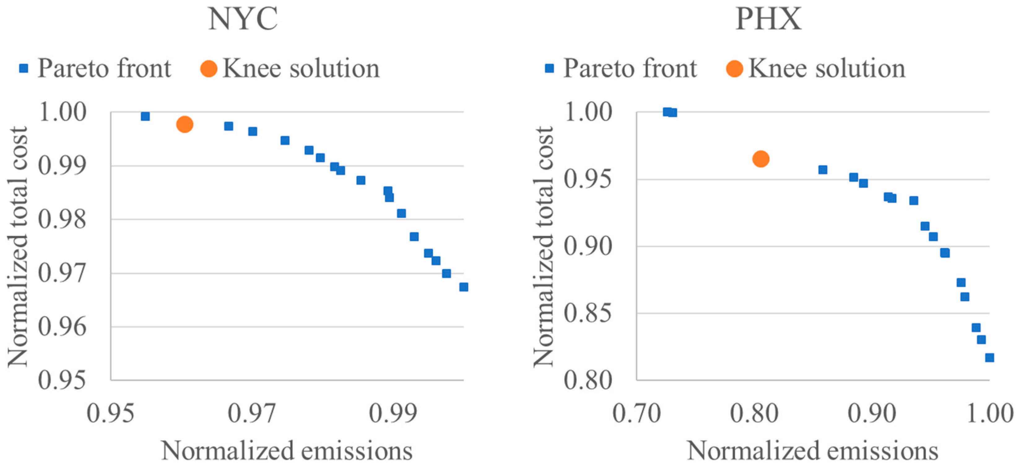
One such “a posteriori” MCDM approach was adopted where the selection of a set of preferred solutions was made by analyzing the knee value [23] of each solution on the Pareto front. Sometimes, the shape of the Pareto-optimal front is such that there may be solutions where a small improvement in one objective will lead to a large deterioration in other objectives, which makes moving in either direction unattractive. For a MOOP that seeks to minimize f1 and f2, the knee value of the ith solution is:
It is necessary to normalize the objective function values while performing knee calculations. The front closest to the origin in Figure 8 was chosen, as it is nondominated. Figure 9 shows the normalized front along with the best knee point. Table 4 contains the solution sets that correspond to the knee values for both locations. Findings corresponding to the general pattern seen in Section 3: n is close to the upper limit and p is of a medium size, with PHX having a larger size than NYC. Charging times are later in the evening, all of which are past 8 PM. This is noteworthy, as solar output is negligible at that time.
4.2. Nearest Point
Another MCDM approach is the ideal point method [24]. Here, the optimizer picks an optimal solution that has the least geometric distance to some reference point, like the ideal point. For a min-min problem, the ideal point is the origin (0, 0). In practice, no solution will produce emissions and total costs that are both zero. However, a point on the Pareto front that is nearest to this point may be considered the most optimal. Again, normalized fronts were used, and the result is shown in Figure 10. The optimal solutions are in Table 4. Again, the values of n are close to the upper limit of 25 kW and p, but the battery storage is significantly smaller. Charging times are mostly later in the evening. Interestingly, both NYC and PHX have a clear trend between t and u. The summer charging time is earlier than the winter charging time. In fact, examining all the solutions indicates that all 20 solutions for NYC and 10 out of 20 solutions for PHX follow this trend.
These comparisons demonstrate why MOGA is a superior method for solving MOOPs. Both the knee point and nearest point represent different solutions, giving the customer flexibility. Of course, any of the Pareto front solutions could be picked, but even MCDM, when correctly applied, maintains a choice. If the best knee point is too expensive, then the second-best or third-best knee points can be explored.
4.3. Comparison of Pareto Fronts
In some cases, it is clearly visually which front is the best. In this case, certain analytical tools or metrics may be used to compare fronts. To illustrate this, consider Figure 2. There is a noticeable change in the winter to summer loads for both locations: around 3500 h for NYC and around 3200 h for PHX. Accordingly, a fifth decision variable, tseason, was added to the residential model. This variable was bounded from 2000 to 4000. The MOGA finds the best time of the year (winter to spring) to change the EV charging time from t to u. After six months or 4380 h, the EV charging time switches back. After running the algorithm again, the plots in Figure 11 were obtained. For comparison, the best fronts from Figure 8 (four decision variables) were also plotted.
For NYC, using a variable charging strategy produces a visibly better front. For PHX, it is not so clear. Two comparison metrics are proposed, as used in previous studies [25,26]. The first metric is the area or size of the dominated space. The size of the dominated space, Sd(A), indicates a measure of how much of the objective space is weakly dominated by the Pareto front, A. For a bi-objective optimization problem (min–min), Sd(A) is calculated by using Equation (7).
where n is the total number of solutions in the front. Note that this is a simple area formula (base × height). A larger size indicates a better front. The second metric is the nonuniformity of the front. The measurement of nonuniformity of a Pareto front, A, is calculated by Equation (8)
where di is the distance between two consecutive solutions along the Pareto front A, and is the average distance. A lower value of D(A) indicates a better distribution of obtained solutions on the Pareto front A. The metrics for all four fronts (after normalization) in Figure 11 are in Table 5. The values are very similar because of the overlap between the fronts. For both locations, the variable season front covers more of the dominated space, ~6% more in both cases. However, the fixed season front is more uniform by ~2% in both cases. Thus, while using a fixed charging time during the year produces a Pareto front with a better distribution, it is clearly dominated by the strategy that has a seasonal charging time. For NYC, the summer-winter transition ranged from 3471 h to 3767 h and for PHX, it ranged from 2609 h to 2667. An earlier transition for PHX is to be expected given the climate and the insolation there in April compared to in NYC.
5. Conclusions
This study presented multiobjective optimization results for a grid-tied residential PV system with battery storage and EV charging. The motivation was to develop a strategy that took real-world customer habits into account to provide customers interested in renewable energy with an effective yet straightforward tool to properly size their components. Customers may be unwilling to be flexible in load scheduling or unwilling to incur additional expenses that come with the electronics required to implement such smart strategies. The strategy here is straightforward, extremely low cost, and easy to implement. By using MOGAs, flexibility is preserved.
The residential PV system model was presented and took the most critical and impactful factors into account. The two objectives considered here were the total cost of the system and the carbon footprint or CO2 emissions. These were shown to be conflicting objectives. Several decision variables were considered in the model, with the size of the PV system being found to have the most significant impact on both objectives. Results for the two locations, New York City and Phoenix, followed general trends in previous studies. The efficacy of the MOGA approach in protecting the consumer from choosing dominated (sub-optimal) solutions was demonstrated. The time of the day during which the consume charged their EV was taken as a variable. In both locations, adopting a seasonal strategy—different charging times in the summer and the winter—was found to improve both objectives. Two MCDM criteria were used to demonstrate how an optimal solution may be picked from the Pareto front. Examples for NYC and PHX were 24.5 kW, 9.9 kWh, 10:49 p.m., 8:55 p.m. (n, p, t, u) and 24.9 kW, 16.9 kWh, 10:53 p.m., 10:58 p.m. (n, p, t, u), respectively. Finally, metrics to compare two similar Pareto fronts were also presented. Using a fixed season strategy for EV charging was found to have more diversity in the front (~2%), but was dominated more by the variable season strategy (~6%).
Future studies can take more or different objective functions into account. The model complexity can also be changed to reflect other interesting and useful scenarios that will help the customer relate to everyday experiences. With the proliferation of solar energy, life cycle data such as the emissions from PV fabrication, transportation, etc. can also be incorporated. Hardware accounts for a significant portion of the residential PV system, so future studies can look at trade-offs involving AC and DC systems, specific types of inverters, etc. Different storage options other than batteries can also be considered.
Funding
This research received no external funding.
Acknowledgments
The author is grateful to the University of Wisconsin-Oshkosh for providing facilities to support this study. The author also acknowledges the collaborative effort of the University of Wisconsin-Platteville, particularly involving Fang Yang and Menasha Utilities.
Conflicts of Interest
The author declares no conflict of interest. Note that the author is also the guest editor of the special issue in which this article appears.
Appendix A
Figure A1.
NREL solar estimator data for New York City, NY [16].
Figure A1.
NREL solar estimator data for New York City, NY [16].

References
- Pörtner, H.-O.; Roberts, D.C.; Masson-Delmotte, V.; Zhai, P.; Tignor, M.; Poloczanska, E.; Mintenbeck, K.; Alegría, A.; Nicolai, M.; Okem, A.; et al. (Eds.) IPCC Special Report on the Ocean and Cryosphere in a Changing Climate. IPCC 2019, in press. [Google Scholar]
- U.S. Environmental Protection Agency. Inventory of U.S. Greenhouse Gas Emissions and Sinks: 1990–2018, EPA 430-R-20-002; U.S. Environmental Protection Agency: Washington, DC, USA, 2020.
- United Nations: Department of Economic and Social Affairs. 68% of the World Population Projected to Live in Urban Areas by 2050, Says UN. Available online: https://www.un.org/development/desa/en/news/population/2018-revision-of-world-urbanization-prospects.html (accessed on 27 May 2020).
- U.S. Energy Information Administration. International Energy Outlook 2019 with Projections to 2050; U.S. Department of Energy: Washington, DC, USA, 2019.
- Asante, D.; He, Z.; Adjei, N.O.; Asante, B. Exploring the barriers to renewable energy adoption utilising MULTIMOORA-EDAS method. Energy Policy 2020, 142, 111479. [Google Scholar] [CrossRef]
- Hesse, H.C.; Martins, R.; Musilek, P.; Naumann, M.; Truong, C.N.; Jossen, A. Economic Optimization of Component Sizing for Residential Battery Storage Systems. Energies 2017, 10, 835. [Google Scholar] [CrossRef]
- Kiptoo, M.K.; Adewuyi, O.B.; Lotfy, M.E.; Senjyu, T.; Mandal, P.; Mamdouh Abdel-Akher, M. Multi-Objective Optimal Capacity Planning for 100% Renewable Energy-Based Microgrid Incorporating Cost of Demand-Side Flexibility Management. Appl. Sci. 2019, 9, 3855. [Google Scholar] [CrossRef] [Green Version]
- Iyengar, S.S.; Lepper, M.R. When Choice is Demotivating: Can One Desire Too Much of a Good Thing? J. Personal. Soc. Psychol. 2000, 79, 995–1006. [Google Scholar] [CrossRef]
- Martins, R.; Hesse, H.C.; Jungbauer, J.; Vorbuchner, T.; Musilek, P. Optimal Component Sizing for Peak Shaving in Battery Energy Storage System for Industrial Applications. Energies 2018, 11, 2048. [Google Scholar] [CrossRef] [Green Version]
- Marcinkoski, J.; Vijayagopal, R.; Kast, J.; Duran, A. Driving an Industry: Medium and Heavy Duty Fuel Cell Electric Truck Component Sizing. World Electr. Veh. J. 2016, 8, 78–89. [Google Scholar] [CrossRef] [Green Version]
- Sampietro, J.L.; Puig, V.; Costa-Castelló, R. Optimal Sizing of Storage Elements for a Vehicle Based on Fuel Cells, Supercapacitors, and Batteries. Energies 2019, 12, 925. [Google Scholar] [CrossRef] [Green Version]
- Sim, K.; Vijayagopal, R.; Kim, N.; Rousseau, A. Optimization of Component Sizing for a Fuel Cell-Powered Truck to Minimize Ownership Cost. Energies 2019, 12, 1125. [Google Scholar] [CrossRef] [Green Version]
- Vijayagopal, R.; Chen, R.; Sharer, P.; Wild, S.M.; Rousseau, A. Using multiobjective optimization for automotive component sizing. World Electr. Veh. J. 2015, 7, 261–269. [Google Scholar] [CrossRef] [Green Version]
- Federal Reserve Bank of St. Louis. Economic Research (Categories>Prices>Commodities>Electricity per kWh. Available online: https://research.stlouisfed.org/ (accessed on 15 May 2020).
- NREL: Renewable Resource Database. National Solar Radiation Data Base. Available online: https://nsrdb.nrel.gov/ (accessed on 19 October 2020).
- NREL: PV Watts® Calculator. Available online: https://pvwatts.nrel.gov/pvwatts.php (accessed on 30 April 2020).
- Open Energy Information. Commercial and Residential Hourly Load Profiles for all TMY3 Locations in the United States. Available online: https://openei.org/datasets/files/961/pub/ (accessed on 30 April 2020).
- Vaz, W.; Nandi, A.K.; Landers, R.G.; Koylu, U.O. Electric vehicle range prediction for constant speed trip using multi-objective optimization. J. Power Sources 2015, 275, 435–446. [Google Scholar] [CrossRef]
- Deb, K.; Pratap, A.; Agarwal, S.; Meyarivan, T. A Fast and Elitist Multiobjective Genetic Algorithm: NSGA-II. IEEE Trans. Evol. Comput. 2002, 6, 182–197. [Google Scholar] [CrossRef] [Green Version]
- U.S. Energy Information Administration. State Electricity Profiles. Available online: https://www.eia.gov/electricity/state/ (accessed on 18 May 2020).
- Ardani, K.; O’Shaughnessy, E.; Fu, R.; McClurg, C.; Huneycutt, J.; Margolis, R. Installed Cost Benchmarks and Deployment Barriers for Residential Solar Photovoltaics with Energy Storage; TP-7A40-67474; NREL (National Renewable Energy Lab.): Golden, CO, USA, 2019.
- Mongird, K.; Fotedar, V.; Viswanathan, V.; Koritarov, V.; Balducci, P.; Hadjerioua, B.; Alam, J. Energy Storage Technology and Cost Characterization Report; PNNL-28866; Pacific Northwest National Laboratory: Richland, WA, USA, 2019.
- Branke, J.; Deb, K.; Dierolf, H.; Osswald, M. Finding knees in multi-objective optimization. In Parallel Problem Solving from Nature; Yao, X., Ed.; Springer: Berlin/Heidelberg, Germany, 2004; pp. 722–731. [Google Scholar]
- Miettinen, K. Interactive methods. In Nonlinear Multiobjective Optimization; Springer: Boston, MA, USA, 1998; pp. 131–213. [Google Scholar]
- Audet, C.; Bigeon, J.; Cartier, D.; Le Digabel, S.; Salomon, L. Performance indicators in multiobjective optimization. Prepr. Submitt. Eur. J. Oper. Res. 2018. Available online: http://www.optimization-online.org/DB_FILE/2018/10/6887.pdf (accessed on 19 October 2020).
- Chakraborty, D.; Vaz, W.; Nandi, A.K. Optimal driving during electric vehicle acceleration using evolutionary algorithms. Appl. Soft Comput. 2015, 34, 217–235. [Google Scholar] [CrossRef]
Figure 1.
Grid-tied residential solar photovoltaic (PV) system with battery storage; arrows represent the flow of electrical energy.
Figure 1.
Grid-tied residential solar photovoltaic (PV) system with battery storage; arrows represent the flow of electrical energy.

Figure 2.
Daily hourly electrical load for (top) NYC and (bottom) PHX.

Figure 3.
Schematic representation of binary-coded NSGA-II for a two-objective problem with one decision variable.
Figure 3.
Schematic representation of binary-coded NSGA-II for a two-objective problem with one decision variable.


Figure 5.
Total cost vs. emissions for NYC and PHX based on a varying solar PV size.

Figure 6.
Total cost vs. emissions for NYC and PHX based on a varying battery storage size.

Figure 7.
Total cost vs. emissions for NYC and PHX for varying EV charging times (t).

Figure 8.
Total cost vs. emissions for NYC and PHX for varying EV charging times (t).

Figure 9.
Normalized fronts with knee solutions.

Figure 10.
Normalized fronts with nearest solutions.

Figure 11.
Comparison of fronts for a variable seasonal charging strategy.


Table 1.
Electricity prices ($/kWh) for New York City (NYC) and Phoenix (PHX) (2019) [14].
Table 1.
Electricity prices ($/kWh) for New York City (NYC) and Phoenix (PHX) (2019) [14].
| Month | New York City | Phoenix |
|---|---|---|
| January | 0.202 | 0.131 |
| February | 0.196 | 0.132 |
| March | 0.201 | 0.130 |
| April | 0.197 | 0.130 |
| May | 0.194 | 0.150 |
| June | 0.211 | 0.149 |
| July | 0.207 | 0.153 |
| August | 0.202 | 0.153 |
| September | 0.205 | 0.149 |
| October | 0.194 | 0.148 |
| November | 0.197 | 0.128 |
| December | 0.193 | 0.128 |
Table 2.
Genetic algorithm parameters.
| Algorithm | NSGA-II |
|---|---|
| Number of objectives | 2 |
| Number of decision variables | 4 |
| Lower/upper limits, n | {1, 25} |
| Lower/upper limits, p | {1, 25} |
| Lower/upper limits, t | {16, 24} |
| Lower/upper limits, u | {16, 24} |
| Population size | 20 |
| Number of generations | 100 |
| Crossover probability | 0.9 |
| Mutation probability | 0.01 |
| Tournament size | 2 |
| Selection type | Crowded tournament * |
* fronts are ranked; if equal, then crowding distance is used.
| Parameter | Value |
|---|---|
| Required solar PV size (n) | Decision variable |
| Power density (Apanel) | 172.5 Wm−2 |
| Correction factor (f) | 0.18 |
| Net metering revenue (rnm) | 0.078 $/kWh |
| Battery charge/discharge efficiency (%) | 90 |
| Battery capacity (p) | Decision variable |
| EV battery capacity | 30 kWh |
| EV charging rate | 2 kW |
| Daily EV energy consumption | 16 ± 6 kWh |
| EV charging time of day (t, u) | Decision variable |
| CO2 emissions (NYC) (ε) | 0.212 kg/kWh |
| CO2 emissions (PHX) (ε) | 0.417 kg/kWh |
| Project lifespan (q) | 25 years |
| Rate of price increase (g) | 1.5% |
Table 4.
Summary of best solutions for NYC and PHX.
| Criterion | Value of Decision Variables |
|---|---|
| Knee (NYC) | 24.5 kW, 9.9 kWh, 10:49 p.m, 8:55 p.m (n, p, t, u) |
| Knee (PHX) | 24.9 kW, 16.9 kWh, 10:53 p.m, 10:58 p.m (n, p, t, u) |
| Ideal point (NYC) | 24.4 kW, 2.9 kWh, 10:30 p.m, 8:50 p.m (n, p, t, u) |
| Ideal point (PHX) | 24.8 kW, 5.8 kWh, 7:05 PM, 5:23 p.m (n, p, t, u) |
Table 5.
Pareto front comparison metrics.
| Front | Sd(A) | D(A) |
|---|---|---|
| Fixed season (NYC) | 8.087 × 10⁻² | 0.979 |
| Variable season (NYC) | 8.618 × 10⁻² | 0.998 |
| Fixed season (PHX) | 2.586 × 10⁻² | 0.965 |
| Variable season (PHX) | 2.763 × 10⁻² | 0.988 |
Publisher’s Note: MDPI stays neutral with regard to jurisdictional claims in published maps and institutional affiliations. |
© 2020 by the author. Licensee MDPI, Basel, Switzerland. This article is an open access article distributed under the terms and conditions of the Creative Commons Attribution (CC BY) license (http://creativecommons.org/licenses/by/4.0/).
Share and Cite
MDPI and ACS Style
Vaz, W.S. Multiobjective Optimization of a Residential Grid-Tied Solar System. Sustainability 2020, 12, 8648. https://doi.org/10.3390/su12208648
AMA Style
Vaz WS. Multiobjective Optimization of a Residential Grid-Tied Solar System. Sustainability. 2020; 12(20):8648. https://doi.org/10.3390/su12208648
Chicago/Turabian StyleVaz, Warren S. 2020. "Multiobjective Optimization of a Residential Grid-Tied Solar System" Sustainability 12, no. 20: 8648. https://doi.org/10.3390/su12208648
Note that from the first issue of 2016, this journal uses article numbers instead of page numbers. See further details here.