Agriculture and Green Economy for Environmental Kuznets Curve Adoption in Developing Countries: Insights from Rwanda

Abstract

Development and climate change are crucial global concerns with significant contrasts between developed and developing nations. Contrary to several developing countries, Rwanda opted for a green growth policy pathway while struggling with its economic emergence through the alternative green sectors, including agriculture. No research has yet been conducted on the choice’s performance on emission sequestration or the country’s income, allowing the formulation of strategies accordingly. The environmental Kuznets curve (EKC), mostly adopted by developed countries, is applied for the Rwandese scenario to verify its adoption in developing countries. The within and between effects of the agricultural sector (AGRc) and gross domestic products (GDPc) on CO₂ emission (CO₂) are examined with an Autoregressive Distributed Lag (ARDL) cointegration and coupling methods in January 2008−December 2018 period. Results confirm the short-run and long-run cointegration relationships of variables, where CO₂-GDPc and CO₂-AGRc are relatively decoupling and absolute decoupling, respectively. The EKC adoption to CO₂-GDPc relationship, and the significant negative causality from GDPc and AGRc to CO₂, are confirmed. The performance resulted from the country’s environment conservation policies, and Rwanda is a learning example as a developing country. However, the green economy through the agro-economy is at a low level and should be reinforced.

1. Introduction

Nowadays, sustainable development and environmental protection are crucial worldwide concerns, where transitions towards sustainable production and consumption are buzzwords [1]. The agriculture sector produces several environmental protection services, including greenhouse gas sequestration. Thus, an agro-economy pathway is a significant green economy promotion, despite several challenges facing the sector, including climate change and its adaptation to technological innovations [2]. A green economy is largely analyzed through the CO₂ emissions with the nexus of income growth determinants [3]; the linkage was revealed by the environmental Kuznets curve (EKC) theory supporting an inverted U-shape relation [4]. That theory assumes that the environment tends to worsen as new economic growth occurs until the income average reaches a specific development point. Thus, the EKC is mostly applicable to developed nations, as the ones that are supposed to be at that point. Consequently, several developing nations argue that it is reasonable for them to anticipate economic growth by environmental degradation as their degradation is minimal compared to the advanced nations [5].

Contrary to several developing countries, after the conception of Rwanda Environment Management Authority (REMA) in 2006 [6], Rwanda prefers the green economy approach, with various environmental conservation policies and specified implementation plans [7,8]. Simultaneously, it strived with emergence through the alternative green economy sectors, including agriculture [9]. The country discouraged environmental degradation activities despite their GDP contribution shares, where their increased by only 1%, while the green economy shares to GDP raised by 4% in 2006–2019 [10]. Meanwhile, the country held stable GDP growth, averaging 7.5% annually in 2000–2018, where the agriculture is a crucial sector offering 30% of the GDP and hiring 70% of the workforce. Moreover, improved farming policies were adopted, and the budget allocated in the sector rose about two times in 2009–2018 [11]. However, its GDP shares decreased from 33% to 28%, the workforce from 88.6% to 69.8% in 2006–2018, and mainly with the unskilled older people [12].

The above contradictions of agriculture performance and green economy initiatives, raised our research concerns to verify the inconsistency causes and significance of those green initiatives on income and green growth. A green economy policy is a low carbon resource-efficient and an alternative model enhancing human welfare by decreasing environmental hazards. It requires an economic transformation to sustainability drivers. This preference is critical for some governments, especially developing countries, having the major challenges of environmental protection while keeping economic stability, as environmental stocks are their main economic providers [13].

The Rwandese green economy and agriculture policies allow scholars to write on this subject. According to Bagstad et al. (2020), Rwanda implemented the ecosystem accounts balancing the income growth with environmental protection [14]. Moreover, Nishimwe et al. (2020), noted that those initiatives mostly elaborated in developed countries allow integrating natural resources into the national accounts system. Thus, the experience could be useful to other countries [15]. Government green and economy monitors also evaluate the policy performance, where the reduction greenhouse gases emission is 2% in 2015–2020 period [16], while 137,500 green jobs for income growth were created [17]. However, Weatherspoon et al. (2019) reveal stunting as a major problem, especially in rural areas, despite the impressive economic growth, thus encouraging the sector’s transformations to improve food production [18]. Furthermore, in forecasting, it was discovered that despite the general agriculture prediction increment, the increment rate is low compared to the preceding years due to several inefficient capability issues. Therefore, a transformation plan for investment promotion and opportunity awareness to the competent workforce was suggested [12].

Beside the literature on Rwanda, several authors also wrote broadly on green economy issues, especially the agro-economy subject while their conclusions are mostly converging with the Rwandese scenarios. Focusing on the landscape analysis and conditions that could support the agriculture sector towards a sustainable status, Marcello et al. (2020) denoted that many transformation strategies are required, including private investment attraction, where policymakers should create an adequate financial profitability environment with favorite legislation, transparency, and infrastructure development [19]. However, with a systematic review of academic contributions on a green economy, it was denoted that no convincing empirical studies established that could adequately engage investors in green sectors, suggesting more empirical researches with mixed and refined methodologies [20].

Preceding scholars wrote on the Rwandese agriculture and green economy performance. However, little concern has been given to investigate the green economy policies’ performance on greenhouse gas emissions sequestration, especially the agriculture sector performance on emission sequestration, to allow for the reformulation of strategies and policies accordingly. Furthermore, as mentioned by the previous literature, a lack convincing empirical studies, including economic models, also restricts that evaluation. Thus, this research applies the theoretical and empirical approaches to overcome the issues, where an ARDL bounds test of cointegration with coupling hypothesis, and ECM causality models on CO₂, AGRc, and GDPc from 2008 to 2018 allow the following aims:

-

Identify whether developing countries with green economy policies like Rwanda could adopt the EKC, mostly adopted by advanced counties. Through the relationship classification between CO₂-GDPc and CO₂-AGRc. As either relative decoupling, absolute decoupling, relative coupling, absolute coupling, or no relationship.

-

Explore the GDPc and AGRc impact on CO₂ emissions;

-

Precise the causality directions through short-run and long-run stability;

-

Classify the existing weaknesses, opportunities, and improvement strategies.

The rest of this paper is designed as follows: Section 2 outlines the material and methods used, including a theoretical and empirical approach that identifies the harmony existence and relationship in agriculture, environmental, and economic growth. Section 3 displays the result followed by the discussion, while the closing part compiles and concludes.

2. Material and Methods

2.1. Theoretical Approach

2.1.1. Green Growth Grants to Agriculture and Economy

Green growth strategies promote environmental externalities favorable for agricultural production and resource management, as they increase carbon sequestration and improve the natural soil matter to yield tangible benefits [21]. Moreover, the green sector becomes a crucial job creation boosting the national incomes [22]. Due to its geographic location and resource availability, there are significant economic benefits for a developing country such as Rwanda to follow a low carbon resource-efficient pathway. This pathway provides significant potential investments for income and environmental benefits [23]. Moreover, the current Rwandese moderate urbanization, similar to other developing nations, allows in advance the future planning towards greened livable cities for sustainable development [24].

2.1.2. Agricultural Grants to Economy and Environment

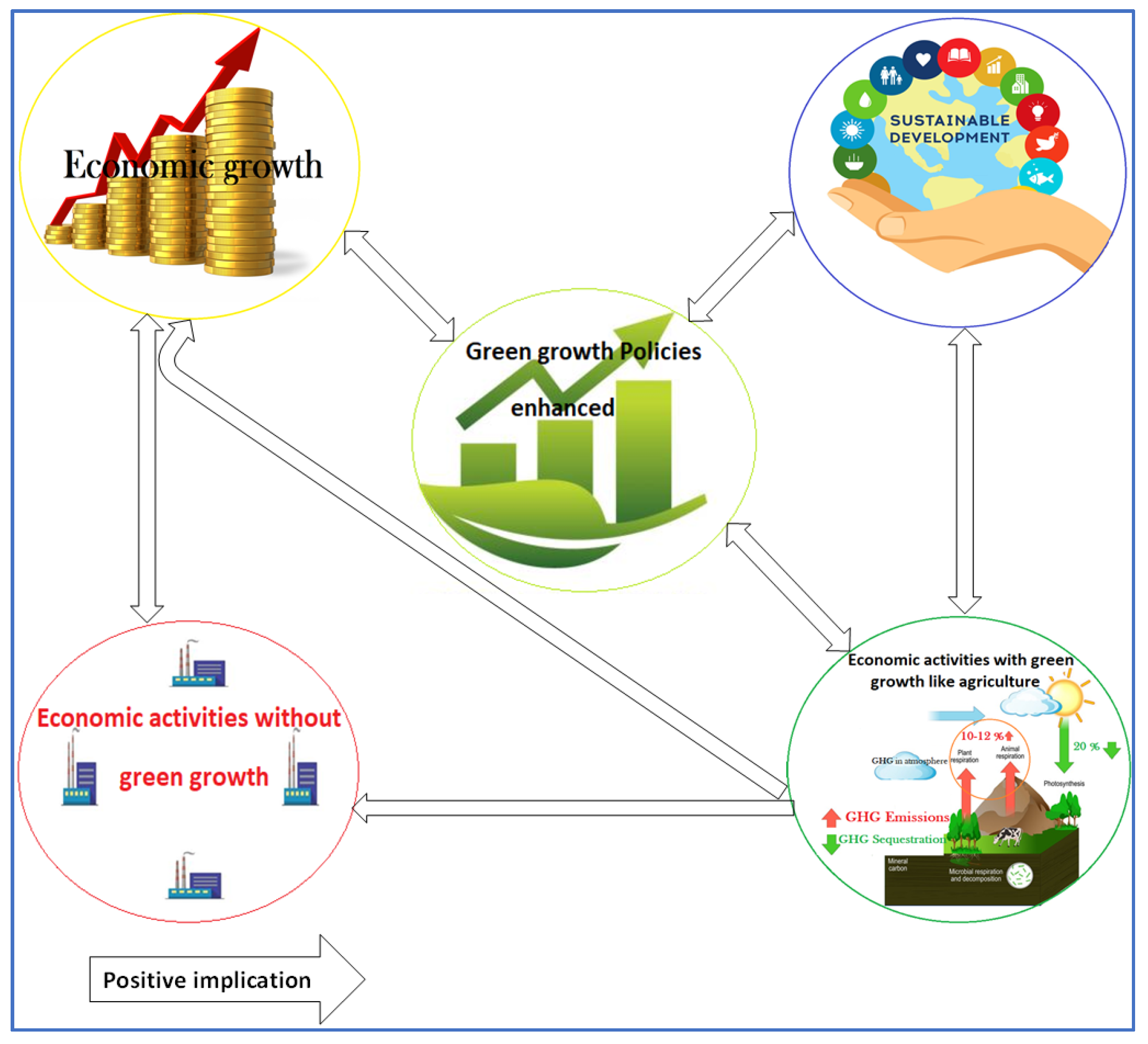
As of 2018, agriculture served only 3% of the world’s economy, dropping from 4% in 2010; despite that small portion, the sector employs almost 30% of the worldwide workers, especially in developing nations [25]. In Rwanda, agriculture contributes 28% of the GDP as of 2018. Thus, an improvement of that economic contributor is not only for social benefit but also for economic welfare [12]. The sector produces a series of environmental assistance necessary for green growth, including greenhouse gas mitigation. The Intergovernmental Panel on Climate Change (IPCC) shows that, although the total direct emissions of agriculture (including livestock and animal species) are about 10–12% of the total global emissions, vegetable, and soil carbon sequestration has the potential to neutralize around 20% of the global greenhouse gases, including CO₂ [26]. Thus, the sector mitigates globally at least 10% of the greenhouse gas emissions. The agriculture area estimates more than 37.7% of the global total land use; adding the forest cover, this rate becomes 68.4%. Moreover, some particular cases like Wang et al. (2015) on the carbon sequestration resulted from the black locust tree, also prove that sequestration scenario [27]. Therefore, the sector performs ecosystem conservation crucial role. The land sector coverage influences the universe by controlling the water and land resources, i.e., plant species, animal habitats, flood control, woodlands, biodiversity preservation, and landscape protection [28]. Figure 1 and the above statements enhance how green growth policies are the intercessor of economic growth, several economic activities, and sustainable development.

2.1.3. Status of Green and No Green Growth Sectors in Rwanda

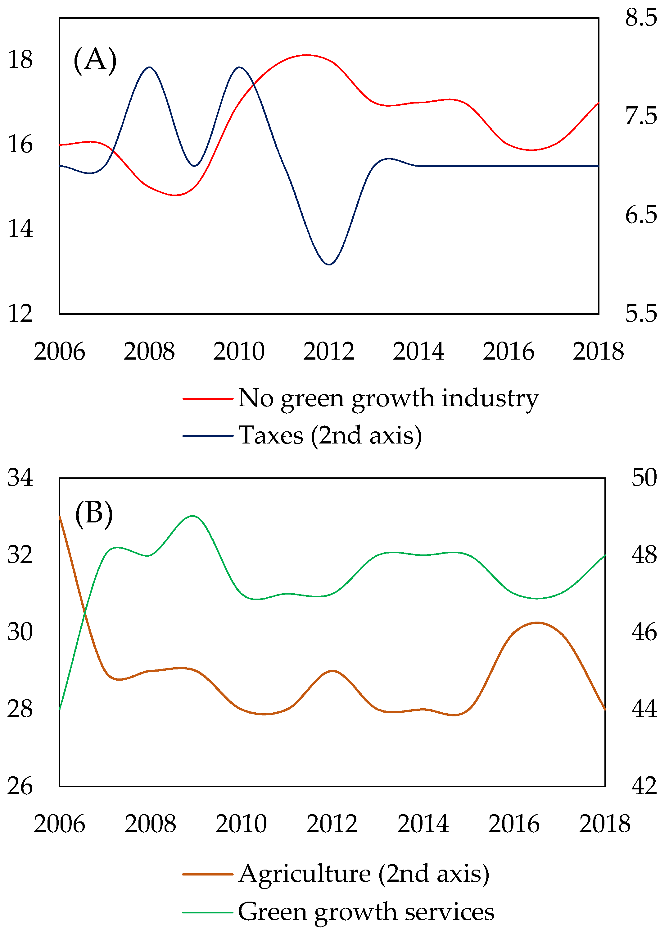
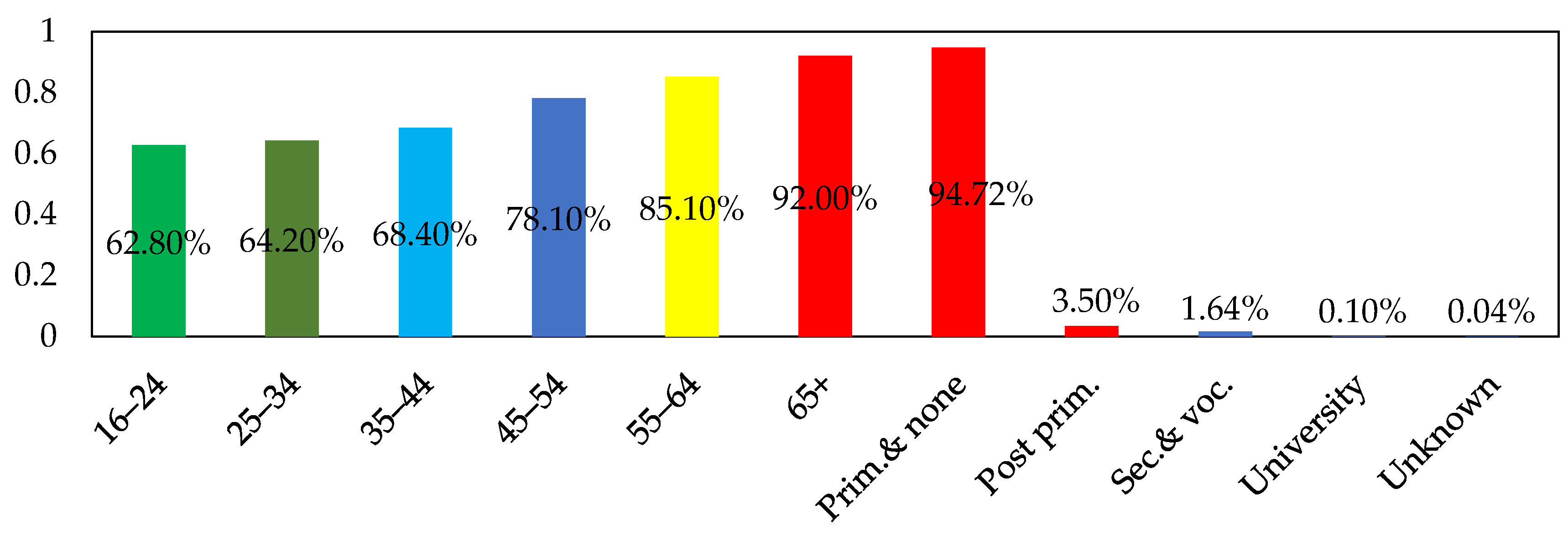
Green growth activities, including agriculture, are the country’s principal economic components offered on an average of 76.4% of the GDP, while the no green sectors gave on average 23.6% in 2006–2018. Only the agriculture sector share was averaging 29% and hired 75.1% of the workforce in that period (

Table 1. Economic contribution proportion by sector from 2006 to 2018.

Sector’s Shares (%)	2006	2008	2010	2012	2014	2016	2018	Average
Agriculture	33	29	28	29	28	30	28	29
Green growth services	44	48	47	47	48	47	48	47.4
No green growth industry	16	15	17	18	17	16	17	16.5
Taxes	7	8	8	6	7	7	7	7.1

Source: National Institute of Statistics of Rwanda (NISR) and author’s calculations.

and

Table 2. Agriculture employment, education levels, and age group proportions 2002–2018.

Years		2002	2006	2010	2014	2018	Average
Employment Proportion %		86.6	79	72.5	67.6	69.8	75.1
Highest level of education
Education levels %		2002	2006	2010	2014	2018	Average
Primary, unknown & none		96.1	96.6	96.6	90.1	94.4	94.76
Post primary		2.3	1.8	1.1	7	5.3	3.50
Secondary & vocational		1.6	1.5	2.1	2.7	0.3	1.64
University		0	0.1	0.2	0.2	0.0	0.10
Age group
Age group	16–24	25–34	35–44	45–54	55–64	65+	Average
percentages	62.8	64.2	68.4	78.1	85.1	92.0	75.1

Source: NISR and author’s calculations.

). However, the agricultural sector decreased from 33% to 28% in 2006–2018 (Figure 2) and mainly comprised of the elderly population with low education levels (Figure 3).

2.2. Description of Variables

This research applied data from the World Bank dataset 2019, the National Institute of Statistics of Rwanda (NISR), the Ministry of agriculture, and Rwanda Environmental Management Authority (REMA). It traced the 132 monthly CO₂, AGRc, and GDPc time series data for the January 2008−December 2018 period, as the green economy enhancement period. Variables structures are presented in Figure 4.

2.3. Model Specification

The aggregated functional form defining the relationship between CO₂, GDPc, and AGRc is:

$${\mathrm{LCO}}_2\left(000\right)=\mathrm{function}\left({\mathrm{LGCF}}_{\mathrm{c}},{ \mathrm{LAGR}}_{\mathrm{c}}\right)$$

(1)

Reflecting on the early analysis a decade ago of [29,30], and the recent with the improved algorithm, including [31,32,33], an appropriate model from Equation (1) is discovered with the following alternative equations:

$${\mathrm{LCO}}_2\left(000\right)={\mathsf{\alpha }}_0+{\mathsf{\alpha }}_1\mathrm{LGDPc}+{\mathsf{\alpha }}_3\mathrm{LAGRc}+{\mathrm{u}}_{\mathrm{i}}$$

(2)

$${\mathrm{LCO}}_2\left(000\right)={\mathsf{\alpha }}_0+{\mathsf{\alpha }}_1\mathrm{LGDPc}+{\mathsf{\alpha }}_{2 }{\mathrm{LGDPc}}^2+{\mathsf{\alpha }}_3\mathrm{LAGRc}+{\mathrm{u}}_{\mathrm{i}}$$

(3)

$${\mathrm{LCO}}_2\left(000\right)={\mathsf{\alpha }}_0+{\mathsf{\alpha }}_1\mathrm{LGDPc}+{\mathsf{\alpha }}_3\mathrm{LAGRc}+{\mathsf{\alpha }}_{4 }{\mathrm{LAGRc}}^2+{\mathrm{u}}_{\mathrm{i}}$$

(4)

$${\mathrm{LCO}}_2\left(000\right)={\mathsf{\alpha }}_0+{\mathsf{\alpha }}_1\mathrm{LGDPc}+{\mathsf{\alpha }}_{2 }{\mathrm{LGDPc}}^2+{\mathsf{\alpha }}_3\mathrm{LAGRc}+{\mathsf{\alpha }}_{4 }{\mathrm{LAGRc}}^2+{\mathrm{u}}_{\mathrm{i}}$$

(5)

LCO₂, LGDPc, and LAGRc are the natural log transform of CO₂, GDPc, and AGRc, respectively. α₁, α₂, α₃, and α₄ are the parameters indicating the CO₂ long and short-term elasticity the regressors. α₀ is the intercept, while u_i is the error term observed as independent and normally distributed with mean zero and constant variance.

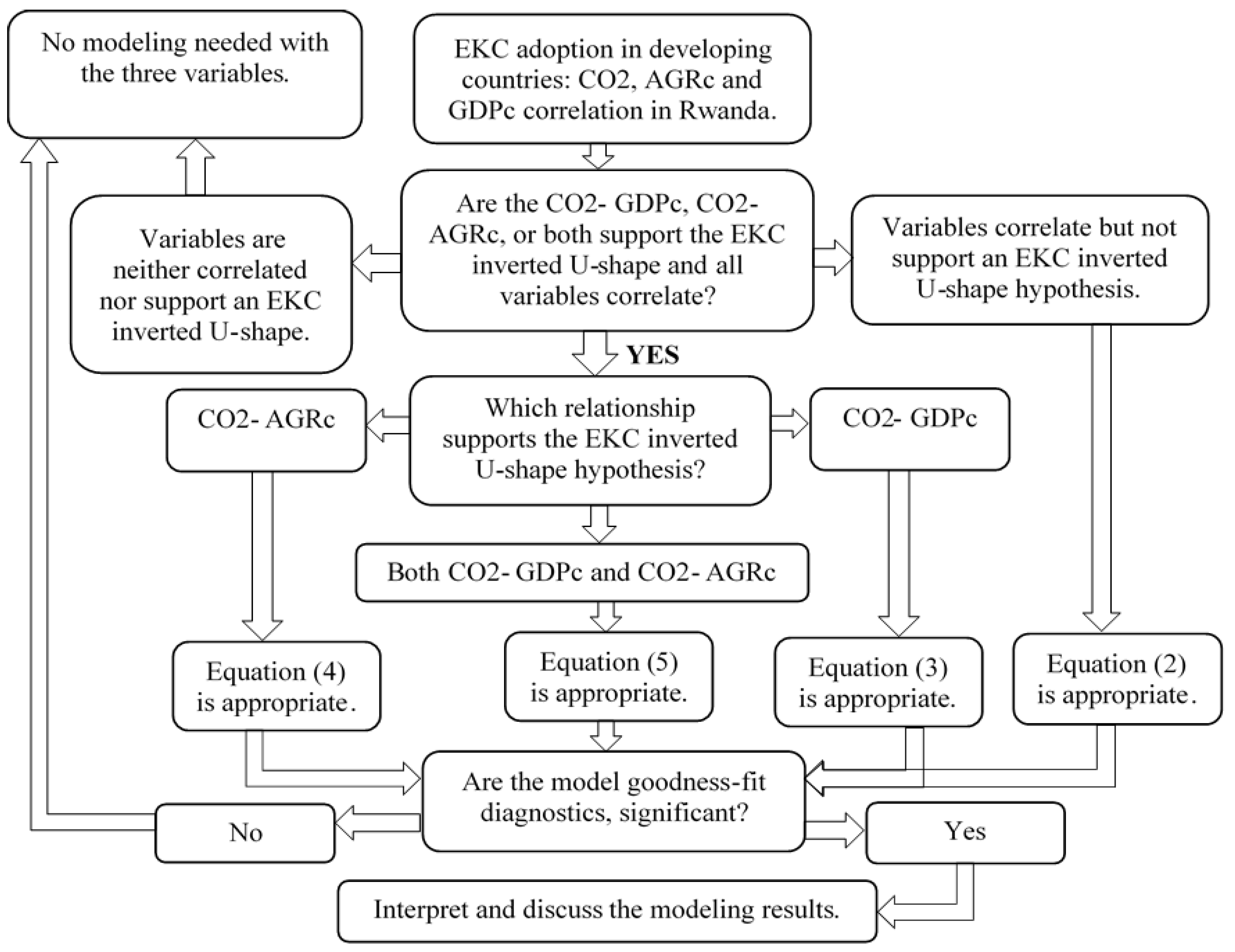
Following the EKC or GBMLQ hypothesis, the turning point occurs alternatively or simultaneously at the agriculture production level of α₃/2α₄ and/or income level of α₁/2α₂. It means that the CO₂ emissions level rise as country income and/or agriculture, then decline as rising income and/or agriculture output pass through the turning point. Figure 5 summarizes the model diagnostics, and testifies the EKC adoption in developing countries.

2.3.1. Tests for the EKC or GBMLQ Inverted U-Shape Hypothesis

Two tests were carried for an inverted U-shape pattern. First, the opposite signs of α₁ to α₂, and α₃ to α₄ or decoupling and coupling scenarios [34]. The coupling and decoupling concept were denoted in terms of CO₂ elasticity from GDPc, and AGRc. If one of the variables increase as the CO₂ goes up, it is a positive CO₂ elasticity. If that positive elasticity is less than unity, the variable increases lower quickly than CO₂, indicating a relative decoupling. For absolute coupling relationship, elasticity is positive and greater nor equal to unity, and regressors increases at the same or large rapidity as the CO₂ (Equation (6)).

$$\begin{gathered} \mathrm{Relative} \mathrm{decoupling}: \frac{{\mathsf{\delta }\mathrm{LCO}}_2}{\mathsf{\delta }\mathrm{LGDPc}}= {\mathrm{g}}^{\prime }\left(\mathrm{LGDPc}\right)<1 \\ \mathrm{Absolute} \mathrm{decoupling}: \frac{{\mathsf{\delta }\mathrm{LCO}}_2}{\mathsf{\delta }\mathrm{LGDPc}}= {\mathrm{g}}^{\prime }\left(\mathrm{LGDPc}\right)<0 \\ \mathrm{Relative} \mathrm{coupling}: \frac{{\mathsf{\delta }\mathrm{LCO}}_2}{\mathsf{\delta }\mathrm{LGDPc}}= {\mathrm{g}}^{\prime }\left(\mathrm{LGDPc}\right)>0 \\ \mathrm{Absolute} \mathrm{coupling}: \frac{{\mathsf{\delta }\mathrm{LCO}}_2}{\mathsf{\delta }\mathrm{LGDPc}}= {\mathrm{g}}^{\prime }\left(\mathrm{LGDPc}\right)>1 \end{gathered}$$

(6)

If the parameters’ signs of linear and quadratic terms are the same, they reveal a monotonic absolute decoupling or coupling relationship among variables, indicating a non-validity of the hypothesis. Otherwise with the optimization rules [33,35], at α₁/2α₂ GDPc level, and/or α₃/2α₄ AGRc level; the turning points occurred when:

$$\begin{gathered} \frac{{\mathsf{\delta }\mathrm{LCO}}_2}{\mathsf{\delta }\mathrm{LGDPc}}=0 \mathrm{iff} \mathrm{LGDPc}=\raisebox{1ex}{${\mathsf{\alpha }}_{1 }$}\!\left/ \!\raisebox{-1ex}{$2{\mathsf{\alpha }}_{2 }$}\right. \\ \frac{{\mathsf{\delta }\mathrm{LCO}}_2}{\mathsf{\delta }\mathrm{LAGRc}}=0 \mathrm{iff} \mathrm{LAGRc}=\raisebox{1ex}{${\mathsf{\alpha }}_{3 }$}\!\left/ \!\raisebox{-1ex}{$2{\mathsf{\alpha }}_{4 }$}\right. \end{gathered}$$

(7)

Second, the R²-adjusted significance produced from the added quadratic terms: To avoid overeating, counterfeit, or both in the regression results, if adding the quadratic term resulted in an adjusted R² that is less than the one in a monotonic equation, it implied a non-validity of the hypothesis. Otherwise, the hypothesis is appropriate [31]. Thus, the modeling analysis was used to define the appropriate Equation either (2), (3), (4), or (5).

2.3.2. ARDL Method for Cointegration

The cointegration precondition is the presence of unit root. Unit roots and variables integration order tests were applied, including Peron Phillips (PP) [36] and Augmented dickey fuller (ADF) [37]. ARDL model contains the lagged value (s) of the dependent variable and the regressors’ current and lagged values as independent variables. If variables are cointegrated from the bounds test, both the long run-VECM and short-run-ARDL models are designated; otherwise, only the short run-ARDL. The long-term and cointegration between variables is the regular OLS regression with the lags of explained and explanatory variables, expressed as ARDL (p, k1, k2… ki). Where p is the explained variable lags number and ki the number of the explanatory variables. A magnetic error correction term is generated in cointegration, connecting the short-run causality in the long run without latter information loss.

The cointegration, EKC, ECM and ARDL approaches have been used by several researchers on economic and green growth variables, including [38], and the recent [39,40]. ARDL is superior to the classical methods, considering its convenience of not reflecting on the variable’s integration of the same order as it can be fitted when variables are at I (0), I (1), or jointly, but not at I (2) or more. It is also more effective in the small and limited sample sizes [32], as is in this research. Thus, the research results from this study could be unbiased. However, as other methods analyzed the secondary data, our methodology’s features could not capture or specify the population or stakeholders’ suggestions and perceptions on the green sector’s investments.

2.3.3. Model Estimation

The generalized ARDL (P, q) is displayed as vectors in Equation (8):

$${\mathrm{Y}}_{\mathrm{t}}={\mathsf{{\rm Y}}}_0+{\displaystyle {\displaystyle \sum }_{\mathrm{i}=1}^{\mathrm{p}}}{\mathsf{\delta }}_{\mathrm{i}}{\mathrm{Y}}_{\mathrm{t}-\mathrm{i}}+{\displaystyle {\displaystyle \sum }_{\mathrm{i}=1}^{\mathrm{q}}}{\mathsf{\beta }}_{\mathrm{i}}{\mathrm{X}}_{\mathrm{t}-\mathrm{i}}+{\mathsf{\epsilon }}_{\mathrm{it}}$$

(8)

where: Y_t and X_i the dependent and independent variables, δ and β the variables coefficients, Υ₀ the intercept, p and q the dependent and independent variables lag, and ε_it the error terms. The explained variable depends on its lagged values, and the current and lagged values of explanatory variables. Thus, the ARDL (p, q₁, q₂, q₃, q₄) cointegration bounds test is:

$$\begin{array}{ll}\mathrm{LC}{\mathrm{O}}_2\left(000\right)=& {\mathrm{a}}_{01}+{\mathrm{b}}_{11}\mathrm{LC}{\mathrm{O}}_2{\left(000\right)}_{\mathrm{t}-\mathrm{i}}+{\mathrm{b}}_{12}\mathrm{L}\mathrm{G}\mathrm{D}\mathrm{P}{\mathrm{c}}_{\mathrm{t}-\mathrm{i}}+{\mathrm{b}}_{13}\mathrm{LGDP}{\mathrm{c}}^2{}_{\mathrm{t}-\mathrm{i}}+{\mathrm{b}}_{14}\mathrm{LAGR}{\mathrm{c}}_{\mathrm{t}-\mathrm{i}}\\ & +{\mathrm{b}}_{15}\mathrm{AGR}{\mathrm{c}}^2{}_{\mathrm{t}-\mathrm{i}}+{\displaystyle {\displaystyle \sum }_{\mathrm{i}=1}^{\mathrm{p}}}{\mathrm{a}}_{\mathrm{i}1}\mathrm{LC}{\mathrm{O}}_{2\mathrm{t}-\mathrm{i}}+{\displaystyle {\displaystyle \sum }_{\mathrm{i}=1}^{\mathrm{q}}}{\mathrm{a}}_{\mathrm{i}2}\mathrm{LGDP}{\mathrm{c}}_{\mathrm{t}-\mathrm{i}}\\ & +{\displaystyle {\displaystyle \sum }_{\mathrm{i}=1}^{\mathrm{q}}}{\mathrm{a}}_{\mathrm{i}3}\mathrm{LGDP}{\mathrm{c}}^2{}_{\mathrm{t}-\mathrm{i}}+{\displaystyle {\displaystyle \sum }_{\mathrm{i}=1}^{\mathrm{q}}}{\mathrm{a}}_{\mathrm{i}4}\mathrm{LAGR}{\mathrm{c}}_{\mathrm{t}-\mathrm{i}}+{\displaystyle {\displaystyle \sum }_{\mathrm{i}=1}^{\mathrm{q}}}{\mathrm{a}}_{\mathrm{i}5}\mathrm{LAGR}{\mathrm{c}}^2{}_{\mathrm{t}-\mathrm{i}}+{\mathrm{e}}_{\mathrm{t}1}\end{array}$$

(9)

The no cointegration null hypothesis is revealed if b_i1 = b_i2 = b_i3 = b_i4 = b_i5, the alternative of cointegration occurs if b_i1 ≠ b_i2 ≠ b_i3 ≠ b_i4 ≠ b_i5, where I = 1 to 5. Equation (8) expresses Y_t as a vector; thus, to test the cointegration, each of the five variables is used as the dependent.

If no cointegration, only the short-term ARDL (p, q₁, q₂, q₃, q₄) model is specified as:

$$\begin{array}{ll}∆\mathrm{LC}{\mathrm{O}}_2\left(000\right)=& {\mathrm{a}}_{01}+{\displaystyle {\displaystyle \sum }_{\mathrm{i}=1}^{\mathrm{p}}}{\mathrm{a}}_{\mathrm{i}1}∆\mathrm{LC}{\mathrm{O}}_2{\left(000\right)}_{\mathrm{t}-\mathrm{i}}+{\displaystyle {\displaystyle \sum }_{\mathrm{i}=1}^{\mathrm{q}1}}{\mathrm{a}}_{\mathrm{i}2}∆\mathrm{LGDP}{\mathrm{c}}_{\mathrm{t}-\mathrm{i}}\\ & +{\displaystyle {\displaystyle \sum }_{\mathrm{i}=1}^{\mathrm{q}2}}{\mathrm{a}}_{\mathrm{i}3}∆\mathrm{LGDP}{\mathrm{c}}^2{}_{\mathrm{t}-\mathrm{i}}+{\displaystyle {\displaystyle \sum }_{\mathrm{i}=1}^{\mathrm{q}3}}{\mathrm{a}}_{\mathrm{i}4}∆\mathrm{LAGR}{\mathrm{c}}_{\mathrm{t}-\mathrm{i}}+{\displaystyle {\displaystyle \sum }_{\mathrm{i}=1}^{\mathrm{q}4}}{\mathrm{a}}_{\mathrm{i}5}∆\mathrm{LAGR}{\mathrm{c}}^2{}_{\mathrm{t}-\mathrm{i}}+{\mathrm{e}}_{\mathrm{t}}\end{array}$$

(10)

If cointegration exists, the ARDL long and short run respectively estimates are:

$$\begin{array}{ll}\mathrm{LC}{\mathrm{O}}_2\left(000\right)=& {\mathrm{a}}_{01}+{\displaystyle {\displaystyle \sum }_{\mathrm{i}=1}^{\mathrm{p}}}{\mathrm{a}}_{\mathrm{i}1}\mathrm{LC}{\mathrm{O}}_2{\left(000\right)}_{\mathrm{t}-\mathrm{i}}+{\displaystyle {\displaystyle \sum }_{\mathrm{i}=1}^{\mathrm{q}1}}{\mathrm{a}}_{\mathrm{i}2}\mathrm{LGDP}{\mathrm{c}}_{\mathrm{t}-\mathrm{i}}+{\displaystyle {\displaystyle \sum }_{\mathrm{i}=1}^{\mathrm{q}2}}{\mathrm{a}}_{\mathrm{i}3}\mathrm{LGDP}{\mathrm{c}}^2{}_{\mathrm{t}-\mathrm{i}}\\ & +{\displaystyle {\displaystyle \sum }_{\mathrm{i}=1}^{\mathrm{q}3}}{\mathrm{a}}_{\mathrm{i}4}\mathrm{LAGR}{\mathrm{c}}_{\mathrm{t}-\mathrm{i}}+{\displaystyle {\displaystyle \sum }_{\mathrm{i}=1}^{\mathrm{q}4}}{\mathrm{a}}_{\mathrm{i}5}\mathrm{LAGR}{\mathrm{c}}^2{}_{\mathrm{t}-\mathrm{i}}+{\mathrm{e}}_{\mathrm{t}1}\end{array}$$

(11)

$$\begin{array}{ll}∆\mathrm{LC}{\mathrm{O}}_2={\mathrm{a}}_{01}+& {\displaystyle {\displaystyle \sum }_{\mathrm{i}=1}^{\mathrm{p}}}{\mathrm{a}}_{\mathrm{i}1}∆\mathrm{LC}{\mathrm{O}}_2{\left(000\right)}_{\mathrm{t}-\mathrm{i}}+{\displaystyle {\displaystyle \sum }_{\mathrm{i}=1}^{\mathrm{q}1}}{\mathrm{a}}_{\mathrm{i}2}∆\mathrm{LGDP}{\mathrm{c}}_{\mathrm{t}-\mathrm{i}}+{\displaystyle {\displaystyle \sum }_{\mathrm{i}=1}^{\mathrm{q}2}}{\mathrm{a}}_{\mathrm{i}3}∆\mathrm{LGDP}{\mathrm{c}}^2{}_{\mathrm{t}-\mathrm{i}}\\ & +{\displaystyle {\displaystyle \sum }_{\mathrm{i}=1}^{\mathrm{q}3}}{\mathrm{a}}_{\mathrm{i}4}∆\mathrm{LAGR}{\mathrm{c}}_{\mathrm{t}-\mathrm{i}}+{\displaystyle {\displaystyle \sum }_{\mathrm{i}=1}^{\mathrm{q}4}}{\mathrm{a}}_{\mathrm{i}5}∆\mathrm{LAGR}{\mathrm{c}}^2{}_{\mathrm{t}-\mathrm{i}}+\mathsf{\lambda }\mathrm{EC}{\mathrm{T}}_{\mathrm{t}-1}+{\mathrm{e}}_{\mathrm{t}2}\end{array}$$

(12)

where ECT_t−1: the error correction term from the cointegrated Equation (9), showing the variables quickness convergence to the equilibrium, λ: the adjustment speed for every shock attempting the long-term equilibrium deviation (λ comes with a negative sign to prove the model convergence in the long term; otherwise, the model is explosive). e_t: serial uncorrelated error term. From Equations (11) and (12) we have:

$$\begin{array}{ll}\mathrm{EC}{\mathrm{T}}_{\mathrm{t}}=\mathrm{LC}{\mathrm{O}}_2-& {\mathrm{a}}_{01}-{\displaystyle {\displaystyle \sum }_{\mathrm{i}=1}^{\mathrm{p}}}{\mathrm{a}}_{\mathrm{i}1}\mathrm{LC}{\mathrm{O}}_2{\left(000\right)}_{\mathrm{t}-\mathrm{i}}-{\displaystyle {\displaystyle \sum }_{\mathrm{i}=1}^{\mathrm{q}1}}{\mathrm{a}}_{\mathrm{i}2}\mathrm{LGDP}{\mathrm{c}}_{\mathrm{t}-\mathrm{i}}- {\displaystyle {\displaystyle \sum }_{\mathrm{i}=1}^{\mathrm{q}2}}{\mathrm{a}}_{\mathrm{i}3}\mathrm{LGDP}{\mathrm{c}}^2{}_{\mathrm{t}-\mathrm{i}}\\ & -{\displaystyle {\displaystyle \sum }_{\mathrm{i}=1}^{\mathrm{q}3}}{\mathrm{a}}_{\mathrm{i}4}\mathrm{LAGR}{\mathrm{c}}_{\mathrm{t}-\mathrm{i}}-{\displaystyle {\displaystyle \sum }_{\mathrm{i}=1}^{\mathrm{q}4}}{\mathrm{a}}_{\mathrm{i}5}\mathrm{LAGR}{\mathrm{c}}^2{}_{\mathrm{t}-\mathrm{i}}\end{array}$$

(13)

The VECM is established if all the alternative equations are cointegrated. Cointegration exists if the bound test F-statistic is greater than the upper critical bound value for the test. If the value is between the minimum and maximum values, there is no conclusion. There is no cointegration in the model if the F-statistic is less than the lower critical bound [41].

2.3.4. Causality

Causality analysis is based on the ARDL-VECM; lagged forms define the variables short term, long term, and joint causality. The short-run explanatory variables t and χ² statistics perform the short-run causal, λ captures the long-run causality, while the regressors F-statistic and t-statistic of the ECT are for joint causal [32]. Cointegration indicates the existence of the causality at least one direction. Once confirmed, the next step is to determine the causality direction, using the ECT identified by the long run VECM.

$$\begin{gathered} \left[\begin{array}{c}∆\mathrm{L}\mathrm{C}{\mathrm{O}}_{2\mathrm{t}}\\ ∆\mathrm{LGDP}{\mathrm{c}}_{\mathrm{t}}\\ ∆\mathrm{LGDP}{\mathrm{c}}^2{}_{\mathrm{t}}\\ ∆\mathrm{LAGR}{\mathrm{c}}_{\mathrm{t}}\\ ∆\mathrm{LAGR}{\mathrm{c}}^2{}_{\mathrm{t}}\end{array}\right]=\left[\begin{array}{l}{\mathsf{\alpha }}_1\\ {\mathsf{\alpha }}_2\\ {\mathsf{\alpha }}_3\\ {\mathsf{\alpha }}_4\\ {\mathsf{\alpha }}_5\end{array}\right]+\left[\begin{array}{ccccc}{\mathsf{\delta }}_{11,1}& {\mathsf{\delta }}_{12,1}& {\mathsf{\delta }}_{13,1}& {\mathsf{\delta }}_{14,1}& {\mathsf{\delta }}_{15,1}\\ {\mathsf{\delta }}_{21,1}& {\mathsf{\delta }}_{22,1}& {\mathsf{\delta }}_{23,1}& {\mathsf{\delta }}_{24,1}& {\mathsf{\delta }}_{25,1}\\ {\mathsf{\delta }}_{31,1}& {\mathsf{\delta }}_{32,1}& {\mathsf{\delta }}_{33,1}& {\mathsf{\delta }}_{34,1}& {\mathsf{\delta }}_{35,1}\\ {\mathsf{\delta }}_{41,1}& {\mathsf{\delta }}_{42,1}& {\mathsf{\delta }}_{43,1}& {\mathsf{\delta }}_{44,1}& {\mathsf{\delta }}_{45,1}\\ {\mathsf{\delta }}_{51,1}& {\mathsf{\delta }}_{52,1}& {\mathsf{\delta }}_{53,1}& {\mathsf{\delta }}_{54,1}& {\mathsf{\delta }}_{55,1}\end{array}\right]\left[\begin{array}{c}∆\mathrm{L}\mathrm{C}{\mathrm{O}}_{2\mathrm{t}-1}\\ ∆\mathrm{LGDP}{\mathrm{c}}_{\mathrm{t}-1}\\ ∆\mathrm{LGDP}{\mathrm{c}}^2{}_{\mathrm{t}-1}\\ ∆\mathrm{LAGR}{\mathrm{c}}_{\mathrm{t}-1}\\ ∆\mathrm{LAGR}{\mathrm{c}}^2{}_{\mathrm{t}-1}\end{array}\right]+\dots \\ +\left[\begin{array}{ccccc}{\mathsf{\delta }}_{11,\mathrm{k}}& {\mathsf{\delta }}_{12,\mathrm{k}}& {\mathsf{\delta }}_{13,\mathrm{k}}& {\mathsf{\delta }}_{14,\mathrm{k}}& {\mathsf{\delta }}_{15,\mathrm{k}}\\ {\mathsf{\delta }}_{21,\mathrm{k}}& {\mathsf{\delta }}_{22,\mathrm{k}}& {\mathsf{\delta }}_{23,\mathrm{k}}& {\mathsf{\delta }}_{24,\mathrm{k}}& {\mathsf{\delta }}_{25,\mathrm{k}}\\ {\mathsf{\delta }}_{31,\mathrm{k}}& {\mathsf{\delta }}_{32,\mathrm{k}}& {\mathsf{\delta }}_{33,\mathrm{k}}& {\mathsf{\delta }}_{34,\mathrm{k}}& {\mathsf{\delta }}_{35,\mathrm{k}}\\ {\mathsf{\delta }}_{41,\mathrm{k}}& {\mathsf{\delta }}_{42,\mathrm{k}}& {\mathsf{\delta }}_{43,\mathrm{k}}& {\mathsf{\delta }}_{44,\mathrm{k}}& {\mathsf{\delta }}_{45,\mathrm{k}}\\ {\mathsf{\delta }}_{51,\mathrm{k}}& {\mathsf{\delta }}_{52,\mathrm{k}}& {\mathsf{\delta }}_{53,\mathrm{k}}& {\mathsf{\delta }}_{54,\mathrm{k}}& {\mathsf{\delta }}_{55,\mathrm{k}}\end{array}\right]+\left[\begin{array}{l}{\mathsf{\lambda }}_1\\ {\mathsf{\lambda }}_2\\ {\mathsf{\lambda }}_3\\ {\mathsf{\lambda }}_4\\ {\mathsf{\lambda }}_5\end{array}\right]\mathrm{EC}{\mathrm{T}}_{\mathrm{t}-1}+\left[\begin{array}{c}{\mathrm{e}}_{\mathrm{t}1}\\ {\mathrm{e}}_{\mathrm{t}2}\\ {\mathrm{e}}_{\mathrm{t}3}\\ {\mathrm{e}}_{\mathrm{t}4}\\ {\mathrm{e}}_{\mathrm{t}5}\end{array}\right] \end{gathered}$$

(14)

Equations (9) and (12) generate an expanded causal test concerning ECT by the combined VECM, where e_t1 to e_t5 are residual, and δ the short-run elasticity parameters (Equation (14)).

2.4. Model Diagnostics

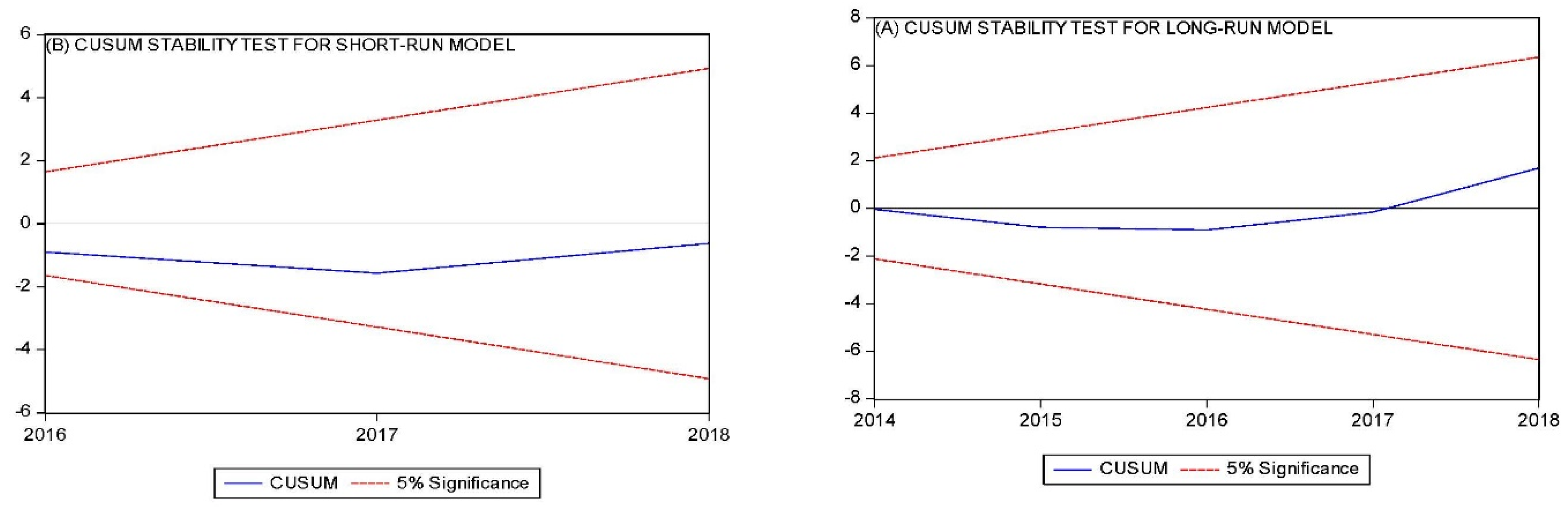
Using the Jarque–Bera (JB) test, the goodness–fit was verified through the heteroscedasticity, serial correlation, Ramsey function, and residuals normality tests. The model stability was tested based on residuals recursive, verified by the Cumulative Sum of Recursive Residuals (CUSUM), represented graphically by two straight lines bounded by the significance level. If the plots slump within the critical significance bounds, the generated regression coefficients are stable, and the null hypothesis of stable coefficients is accepted [4].

3. Data Analysis and Discussion

3.1. Data Analysis

3.1.1. Summary Statistics

This research used annual data on agriculture production, CO₂ emissions, and the real GDP from 2008 to 2018. CO₂ emissions are calculated in metric tons, while the GDPc and agriculture production are in US dollars at 2010 prices (

Table 3. Statistics of variables in summary, 2008–2018.

Variables Statistics	GDPc	AGRc	CO2 (000)
Mean	671.2521	175.2087	66.0352
Standard deviation	93.9015	15.3508	6.1827
Coefficient of variation CV (%)	13.9890	8.7614	9.3627

Source: author’s calculations.

).

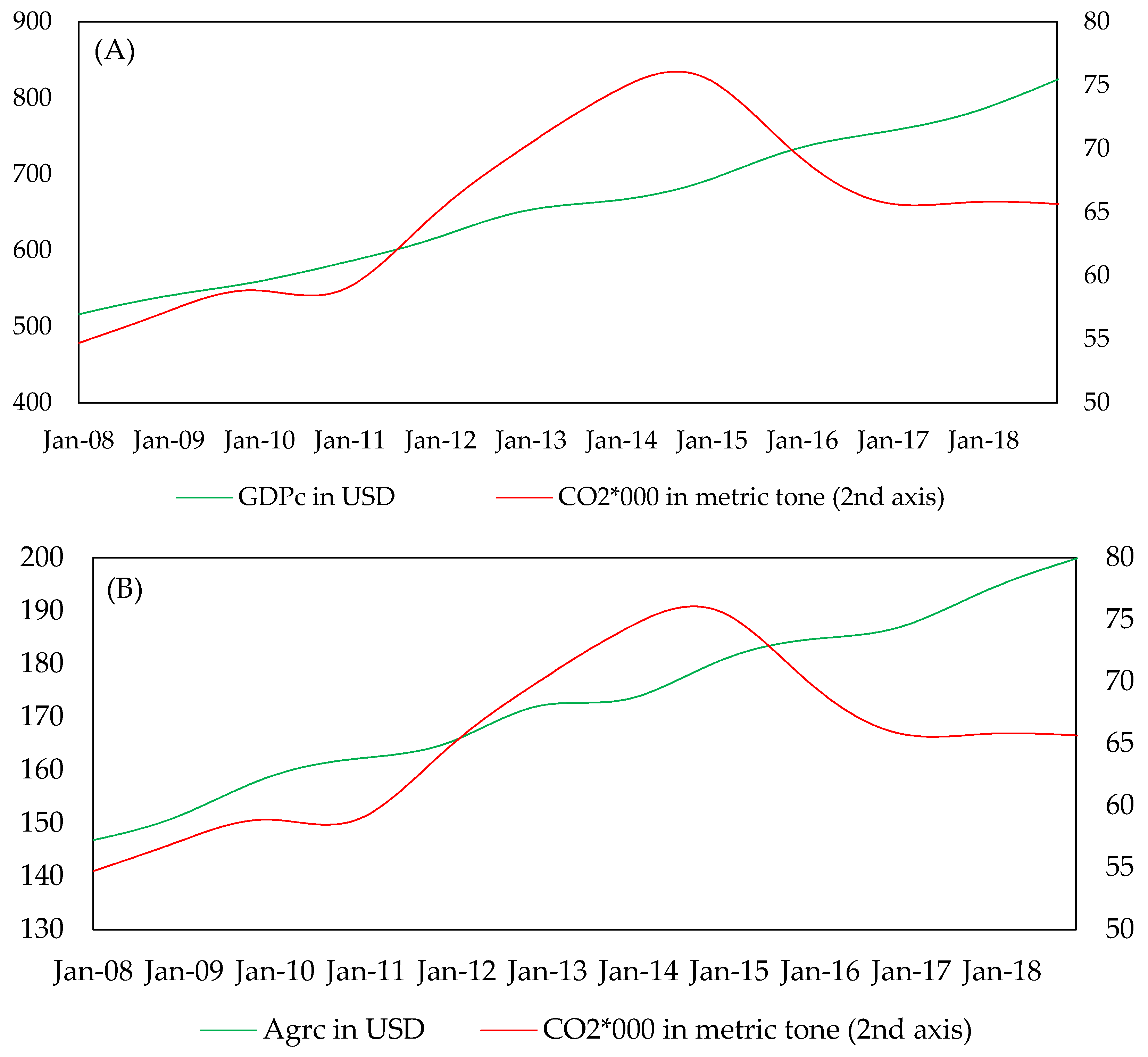
Figure 4 shows the change in Rwanda’s GDPc-CO₂ and AGRc-CO₂ trends. GDPc and AGRc variables increased with CO₂ up to the EKC turning point, then CO₂ trends negatively. However, the agriculture sector’s coefficient of variation (CV) is at a low rate (Table 3).

Table 4. Variable average and compound annual growth rates in East African Community (EAC) 2008–2018.

Country	Years	Variables	Average Annual Growth Rates (AAGR in %)	Compound Annual Growth Rates (CAGR %)
Rwanda	(2008–2013)	GDPc	4.30	4.29
		AGRc	2.79	2.78
		CO2 (000)	5.50	5.45
	(2013–2018)	GDPc	4.42	4.41
		AGRc	2.90	2.89
		CO2 (000)	−2.31	−2.38
Burundi	(2008–2013)	GDPc	1.17	1.17
		AGRc	−1.29	−1.35
		CO2 (000)	5.48	5.29
	(2013–2018)	GDPc	−2.76	−2.79
		AGRc	−4.18	−4.20
		CO2 (000)	18.80	17.59
Kenya	(2008–2013)	GDPc	2.85	2.84
		AGRc	0.97	0.90
		CO2 (000)	3.04	2.62
	(2013–2018)	GDPc	3.09	3.09
		AGRc	2.02	2.01
		CO2 (000)	2.09	1.92
Tanzania	(2008–2013)	GDPc	3.04	3.04
		AGRc	0.21	0.21
		CO2 (000)	9.79	9.45
	(2013–2018)	GDPc	3.22	3.21
		AGRc	2.64	2.64
		CO2 (000)	5.69	5.59
Uganda	(2008–2013)	GDPc	2.53	2.51
		AGRc	−0.86	−0.87
		CO2 (000)	5.73	5.41
	(2013–2018)	GDPc	1.31	1.31
		AGRc	−0.97	−0.97
		CO2 (000)	1.68	1.60

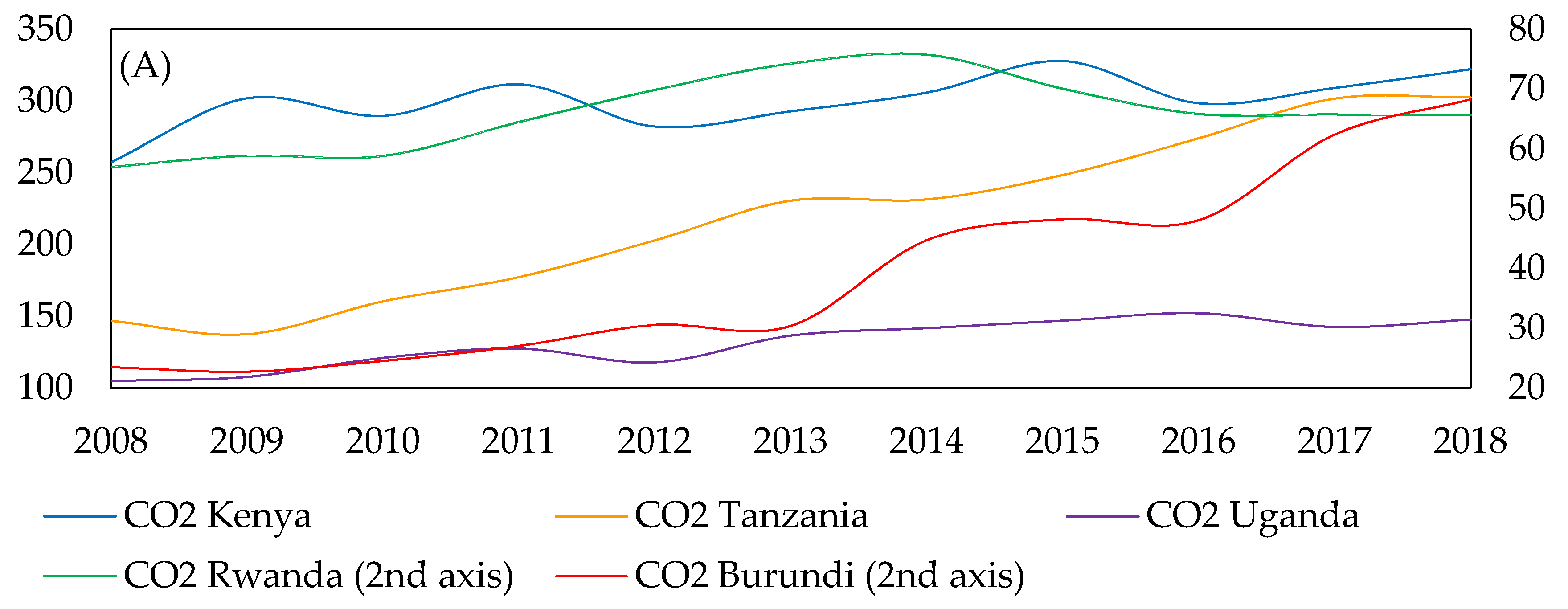
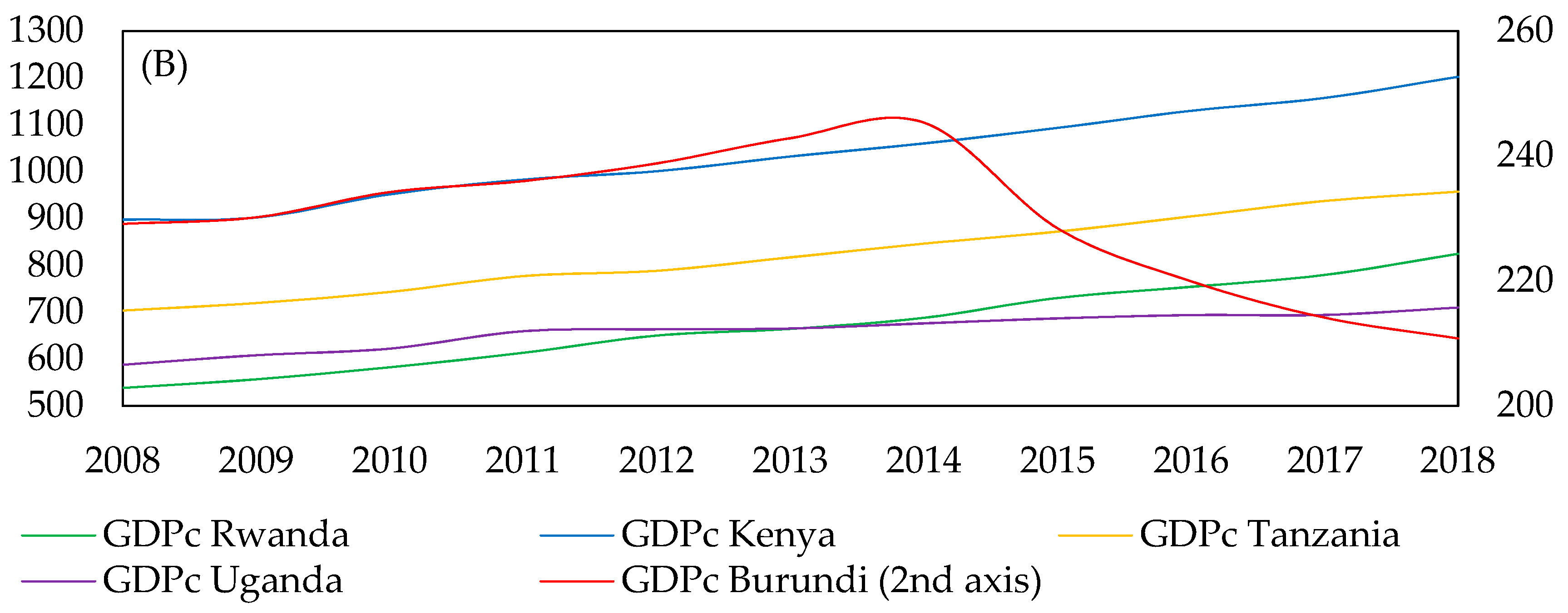
Source: author’s calculations.

compares Rwanda with the neighboring developing nations in the same East African Community (EAC) regional integration, where green growth is not yet adopted (Figure 6).

In (2013–2018) period, the Rwandese AAGR and CAGR of GDPc rounded 4.4%, almost 1.42 times higher than the Kenyan, the best economic performer in EAC, the AAGR, and CAGR rates of AGRc were 2.9%, approximately 1.45 times higher than the regional best performer country. Moreover, Rwanda’s CO₂ growth rate was reduced by around 2.3%, while, in all other EAC countries, it raised by around 18%, 2%, 6%, and 2% for Burundi, Kenya, Tanzania, and Uganda, respectively. Despite the Rwandese GDPc growth with emission reduction (Figure 6), the AGRc growth rates remained almost 1.5 times less than the GDPc. Therefore, for the last 10 years, the increase of Rwandese green growth activities made significant gains in CO2 emissions reduction with a high increment of the GDPc than AGRc (Table 4).

3.1.2. Lag Selection

The variables interdependency is rarely immediate; X reacts to Y with a lapse of time called lag. Extra lags cause degrees of freedom loss, leading to statistically insignificant and can cause multicollinearity. Few lags lead to misspecification errors. Randomly: for annual data, the lag is 1 to 2, quarterly 1 to 8, and monthly 1 to 24 [42]. In this research, the preferred lag length is one. The chosen lag in this paper is one (

Table 5. Variables lag length.

Lag	LogL	LR	FPE	AIC	SC	HQ
0	232.1130	NA	0.001799	−3.482642	−3.394849	−3.446968
1	554.3840	619.9412 *	1.33 × 10−5 *	−8.387543 *	−8.277802 *	−8.342950 *
2	156.0872	65.3826	2.64 × 10−17	−27.2174	−26.6123	−27.8813

Source: author’s calculations.

) (* shows the chosen lag by HQ: Hannan-Quinn information criterion, LR: sequentially modified LR test statistic, FPE: Final prediction error, AIC: Akaike information criterion, and SC: Schwarz information criterion).

3.1.3. Cointegration Test

The bounds test ARDL is appropriate if the descriptive variables are at I (0), I (1) or mutually, and notably none of the variables is at I (2) or above.

ADF and PP tests are consistent with no stationary variables (unit root) at the level, and stationary at I (1). Hence, the ARDL bounds test for cointegration could proceed (

Table 6. The variables unit-roots tests.

Tests	ADF		PP
	Level	1st Diff.	Level	1st Diff.
LCO2 (000)	−2.19	−1.54 *	0.61	−1.62 *
LGDPc	−0.0026	−4.51 **	0.40	−4.77 ***
LGDPc2	0.18	−4.87 ***	0.91	−5.05 ***
LAGRc	0.06	−6.48 ***	−1.24	−14.13 ***
LAGRc2	0.21	−6.51 ***	−0.93	−13.00 ***

***, **, * indicates the H₀ rejection of a unit root in the series at 1%, 5%, and 10%, respectively. Source: author’s calculations.

).

3.1.4. Relevant Equation for the Model

The appropriated equation among (2)–(5) is established through the verification of EKC inverted U-shape hypothesis and cointegration bounds test (Figure 6).

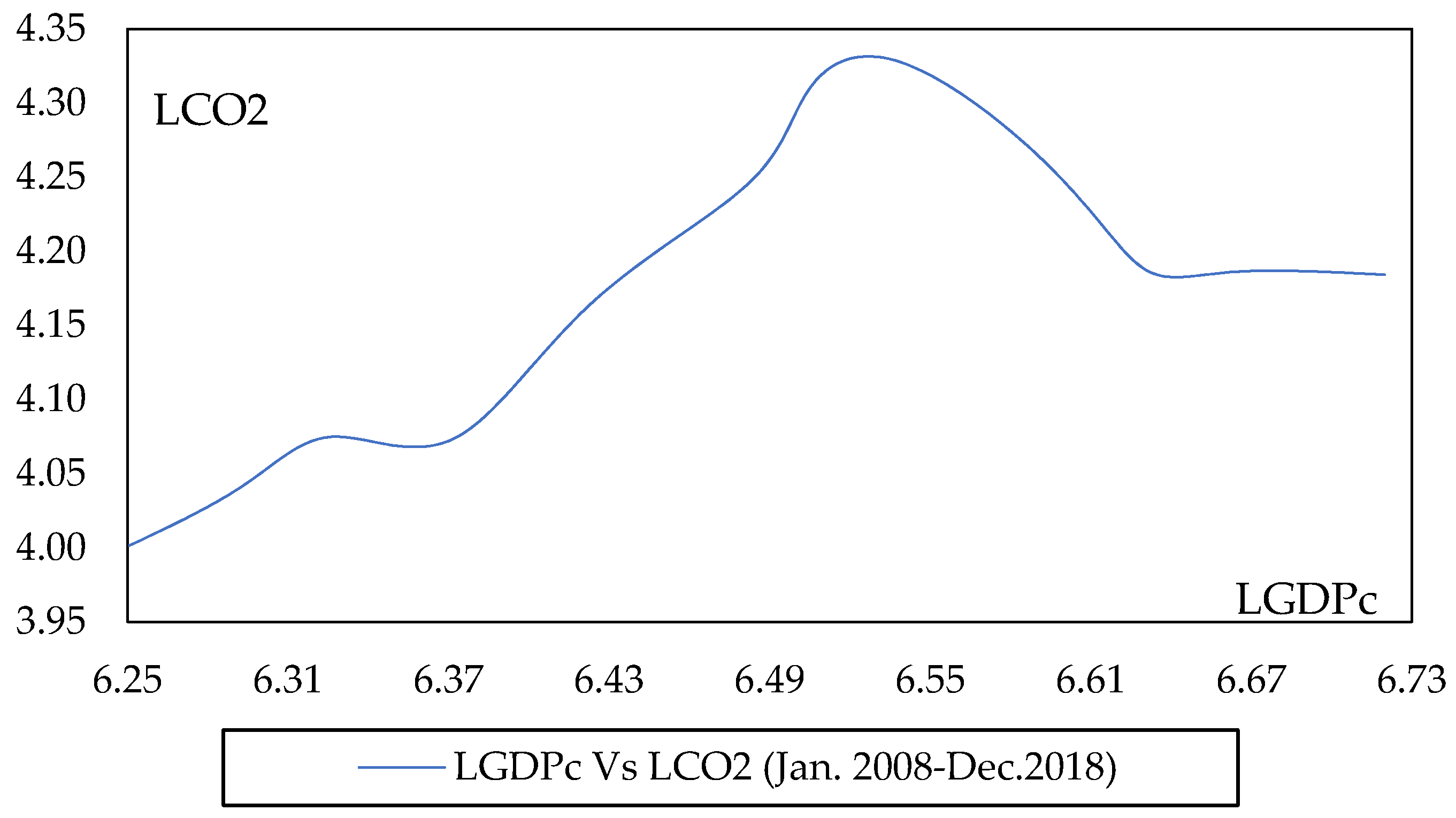
Adding a quadratic term LGDPc² on the linear form results on an adjusted R² greater than 10% and higher than other alternatives options in differences; thus, Equation type (3) is (

Table 7. CO₂ relevant equation type selection.

Equation	Independent Variables				Intercept	Test Statistic
	LGDPc (−1)	LGDPc2 (−1)	LAGRc (−1)	LAGRc2 (−1)		R2-Adjusted	R2-Adjusted Comparison
Equation (2)	0.145659		0.516941		0.575084	0.425584
Equation (3)	50.65348	−3.842931	−0.667313		−159.1832	0.885569	(3)-(2) = 39%
Equation (4)	1.131848		79.42100	−7.821303	−204.6764	0.737725	(4)-(2) = 31.21%
Equation (5)	149.9745	−11.57183	−183.8918	17.92589	−10.06670	0.882306	(5)-(3) = 6.67%

Source: author’s calculations.

). The turning point of inverted U-shape is at around an income level of 6.59 in natural logarithm (=50.65348/(2 × 3.842931) in December 2015. Therefore, only the CO₂-GDPc relationship describes an EKC inverted U-shape (Figure 7), while the CO₂–AGRc relationship presents a monotonic, where the AGRc increases at the expenses of CO₂.

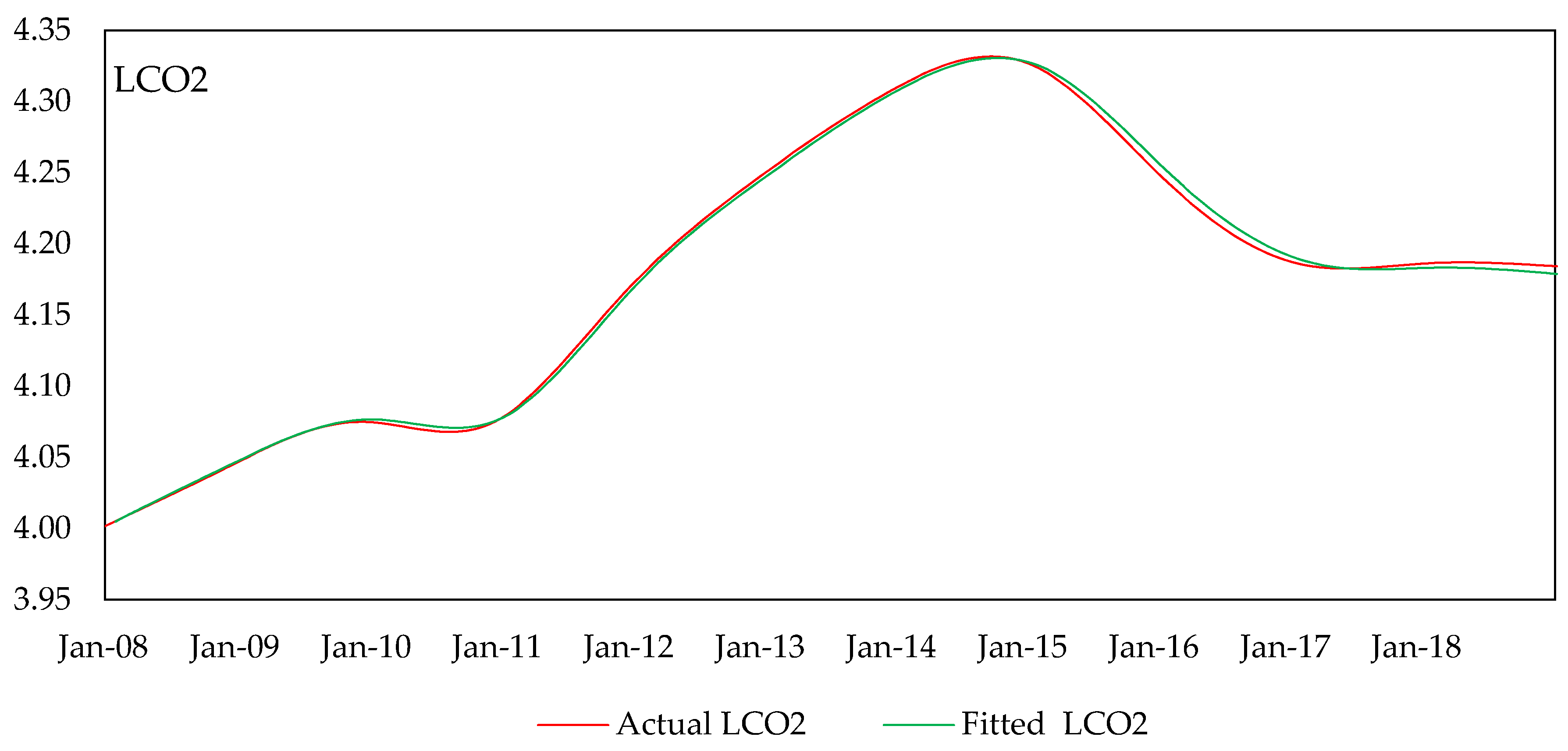
Results show that the F-statistic equal to 11.3278 is higher than the upper bound values at 1%, 5%, and 10% levels, respectively, and alternatives functions are also cointegrated (

Table 8. Bounds test for cointegration with relevant equation.

Function	F-Statistic Value	Lags	Significance Levels			Cointegrated
			Levels	Lower Bound I (0)	Upper Bound I (1)
LCO2(000) = F (LGDPc, LGDPc2, LAGRc)	11.3278	1, 1, 1, 1	10%	2.72	3.77	Yes
			5%	3.23	4.35
			1%	4.29	5.61
LGDPc = F(LCO2(000), LGDPc2, LAGRc)	916.1651	1, 1, 1, 1	10%	2.72	3.77	Yes
			5%	3.23	4.35
			1%	4.29	5.61
LGDPc2 = F(LCO2(000), LGDPc, LAGRc)	921.6545	1, 1, 1, 1	10%	2.72	3.77	Yes
			5%	3.23	4.35
			1%	4.29	5.61
LAGRc = F(LCO2(000), LGDPc, LGDPc2)	6.0842	1, 1, 1, 1	10%	2.72	3.77	Yes
			5%	3.23	4.35
			1%	4.29	5.61

Source: author’s calculations.

). Thus, the no cointegration null hypothesis is rejected at all those levels. The model’s R2 is 99.8% (

Table 9. Results of the model diagnostic tests.

Long-Run Model Diagnostic Tests					Short-Run Model Diagnostic Tests
Residual diagnostics	Serial Correlation	Breusch-Godfrey LM test	R2 observed	3.0980 ** (0.0784)	Serial Correlation	Breusch-Godfrey LM test	R2 observed	7.0933 (0.0077)
		Q-statistic probability	Q-stat.	0.3570 ** (0.5500)		Q-statistic probability	Q-stat.	4.7167 * (0.0300)
	Heteroskedasticity	Breusch-Pagan test	R2 observed	5.2116 ** (0.3654)	Heteroskedasticity	Breusch-Pagan test	R2 observed	6.0445 *** (0.3018)
Stability diagnostics	Miss specification test	Ramsey’s test	t-statistic	1.9555 *** (0.1222)	Miss specification test	Ramsey’s test	t-statistic	0.5397 *** (0.6435)
			F-statistic	3.8243 *** (0.1222)			F-statistic	0.2912 *** (0.6435)
	Recursive estimation	CUSUM	5% level	Results within 5% level	Recursive estimation	CUSUM	5% level	Results within 5% level

*, **, and *** are the no rejection of the null hypothesis of no serial correlation, no heteroskedasticity, or no model miss specification presence at 10%, 5%, and 1% levels of significance, respectively, where the () values are the p-values. Source: author’s calculations.

), indicating that 99.8% of the dependent variable is explained by the regressors. The fitted and actual graphs are closely related (Figure 8).

With the EKC hypothesis, LGDPc and LGDPc² are with parameters α1 > 0 and α2 < 0 in both long term and short-term connections. Thus, the ARDL (1, 1, 1, 1) long-run cointegrated equation is:

$$\begin{gathered} {\mathrm{LCO}}_2\left(000\right)=-5.9431+0.9778{\mathrm{LCO}}_2\left(000\right)\left(-1\right)+2.0075 {\mathrm{LGDP}}_{\mathrm{c}}\left(-1\right) \\ -0.1486{\mathrm{LGDP}}_{\mathrm{c}}^2\left(-1\right)-0.1414{\mathrm{LAGR}}_{\mathrm{c}}\left(-1\right)+{\mathrm{u}}_{\mathrm{i}} \end{gathered}$$

(15)

Thus;

$$\begin{gathered} {\mathrm{LCO}}_2=-0.0059431+0.9972{\mathrm{LCO}}_2\left(-1\right)+0.0020075{\mathrm{LGDP}}_{\mathrm{c}}\left(-1\right) \\ -0.0001486{\mathrm{LGDP}}_{\mathrm{c}}^2\left(-1\right)-0.0001414{\mathrm{LAGR}}_{\mathrm{c}}\left(-1\right)+{\mathrm{u}}_{\mathrm{i}} \end{gathered}$$

(16)

While the ARDL (1, 1, 1, 1) short-run equation is:

$$\begin{gathered} ∆{\mathrm{LCO}}_2{\left(000\right)}_{\mathrm{t}}=0.000491+0.9972∆{\mathrm{LCO}}_2{\left(000\right)}_{\left(-1\right)}+0.8673∆{\mathrm{LGDPc}}_{\left(-1\right)} \\ -0.671∆{\mathrm{LGDPc}}_{\left(-1\right)}^2-0.2178∆{\mathrm{LAGRc}}_{\left(-1\right)}+{\mathrm{u}}_{\mathrm{i}} \end{gathered}$$

(17)

Thus;

$$\begin{gathered} ∆{\mathrm{LCO}}_{2\mathrm{t}}=0.000000491+0.9972∆{\mathrm{LCO}}_2{\left(000\right)}_{\left(-1\right)}+0.0008673∆{\mathrm{LGDPc}}_{\left(-1\right)} \\ -0.000671∆{\mathrm{LGDPc}}_{\left(-1\right)}^2-0.0002178∆{\mathrm{LAGRc}}_{\left(-1\right)}+{\mathrm{u}}_{\mathrm{i}} \end{gathered}$$

(18)

3.1.5. Residual Diagnostics

The process includes the serial correlation and residual heteroskedasticity tests. The serial correlation explains the relationship between the same variable perceptions across precise periods. If it is zero, there is no serial correlation, and the observations are independent of each other. Otherwise, there is a serial correlation where future observations are affected by past values, and the model is not entirely accurate. It occurs if the errors affiliated with a given period move over toward the coming periods [4]. As in Table 9, the no serial correlation hypothesis is accepted, confirming the independence of each observation.

Heteroskedasticity occurs when the variable’s standard errors observed over a specific time are not constant, which is a violation of the regression modeling theories. In this paper, the no heteroskedasticity null hypothesis in both long term and short-term models is accepted. Thus, the variance residual is the same in the model (Table 9).

3.1.6. Stability Diagnostic

Stability diagnostic includes the test for model misspecification and recursive estimation. In this research, it is done through Ramsey’s test to verify whether the fitted combination values explain the dependent variable correctly. The model is mis-designated if another function form might be better to approximate the model. The null hypothesis of no misspecification is not rejected for both long and short-run models (Table 9), reinforcing our choice of Equation (3) type. On the recursive estimation, coefficients are checked for recursive estimates through the CUSUM test (Table 9); the intuition is that the series changes in structural data may be subjected to one or more structural splits [4]. The model stabilities results are within the two straight lines bounded by the 5% level, indicating the model recursive stability (Figure 9). Thus, the given regression ensures the best model fit.

3.1.7. Causality

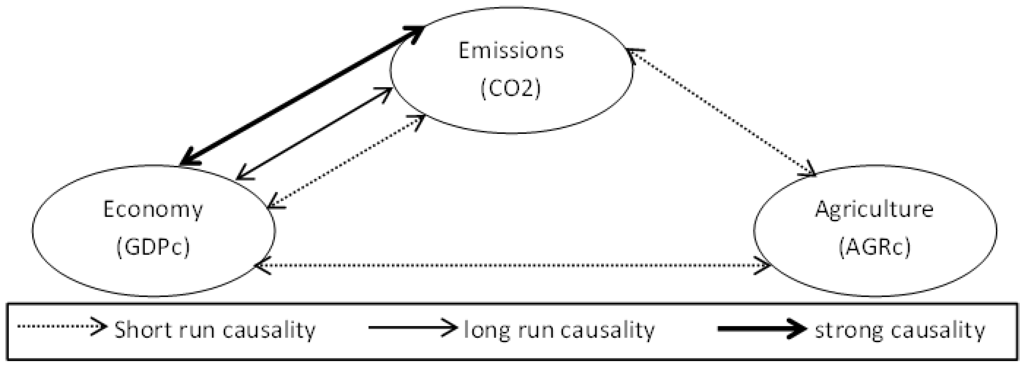
Causality means that the occurrence of X makes an occurrence of Y or vice versa. Thus, the cointegration indicates a causality presence in one direction, at least. It does not make a precision on its direction [33]. The ECM obtained from the long term cointegration is used for causality direction (Figure 10,

Table 10. Long-term, short-term, and VECM estimates.

Variables	Coefficients	Std. Error	t-Statistic	p	R-Squared
Long-run estimates
LCO2(000) (−1)	0.977798	0.007480	130.7264 ***	0.0000	0.9987
LGDPc (−1)	2.007458	0.456357	4.398879 ***	0.0000
LGDPc2 (−1)	−0.148602	0.034636	−4.290376 ***	0.0000
LAGRc (−1)	−0.141488	0.036465	−3.880119 ***	0.0002
Intercept	−5.943106	1.438350	−4.131891 ***	0.0001
Short-run estimates
∆LCO2(000) (−1)	0.997164	0.008312	119.9664 ***	0.0000	0.9939
∆LGDPc (−1)	0.867327	0.480245	1.806010 *	0.0733
∆LGDPc2 (−1)	−0.067058	0.036874	−1.818578 *	0.0714
∆LAGRc (−1)	−0.217765	0.028477	−7.647130 ***	0.0000
Intercept	0.000491	0.000114	4.294216 ***	0.0000
VECM estimates
∆LCO2(000) (−1)	0.983190	0.027120	36.25342 ***	0.0000	0.9939
∆LGDPc (−1)	1.319094	0.963334	1.369301 **	0.0334
∆LGDPc2 (−1)	−0.101936	0.074272	−1.372482 **	0.0324
∆LAGRc (−1)	−0.223091	0.030204	−7.386247 ***	0.0000
ECTt−1	−0.016356	0.030205	0.541490 **	0.0291
Intercept	0.000523	0.000129	4.041930 ***	0.0001

*, **, *** are the significance of values at 1% levels. Source: author’s calculations.

).

3.2. Discussion

Green growth policy allowed Rwanda to mitigate CO₂ emissions considerably while striving with economic emergence. Lighting from the EKC fundamental theory, the CO₂-GDPc short and long-run relations described are on an inverted-U shape curve, where the coefficient associated with the linear term of CO₂ is positive, while its associated on the quadratic term CO₂ is negative. Thus, the Rwandese CO₂-GDPc relationship supports the EKC theory [43], mostly applicable for developed countries, where the CO₂ would increase within the income growth first phase and decrease after achieving a specific point (Figure 7).

Agricultural sector, as one of the green economy alternative sectors, is not only an economic growth contributor but also a green growth promoter for the ecosystem conservation scenarios, including the sequestration of around 10% of the greenhouse gases. Outcomes reveal that the EKC adoption in developing countries with green growth policy like in Rwanda where the agriculture sector is among the principal economic components is feasible, despite its several weaknesses, including shares decrement to GDP, and workforce weaknesses (Table 2).

From 2013 to 2018, the Rwandese, growth rates compared to the neighboring countries in GDPc and AGRc occurred almost 1.42 and 1.45 times higher, respectively, than the region economic best performer. Emissions growth rate reduced by around 2.3%, while in all other regional integrated EAC countries, that growth rates increased. Thus, with a green growth policy, Rwanda shows income growth and environmentally protected significantly (Figure 6). The 2008–2018 Rwandese GDPc coefficient of variation (CV) was 14%, greater than the ones for all other EAC countries with no reinforced green policies (Table 3). It means that the green policy reinforcement in developing countries does not imply a decrease in income. Instead, when it is well managed with alternative green economy activities, it generates an economic boosting.

With lag one, data structure, and cointegration conditions (Table 6), the ARDL is the appropriate model for this research with variables short-run and short-run long-run correlations. Furthermore, the elaborated tests reveal that the estimated values support an EKC hypothesis at the CO₂-GDPc relationship, where the respective long run and short run appropriate equations are (16) (18). Explained as holding other terms constant: In both long and short-run relationships, the GDPc provides a positive and negative elasticity, to the CO₂, while the AGRc-CO₂ is a monotonic negative relationship (Table 10). In the long run, before the EKC turning point, the 1% rose in GDPc results on 0.0020075% increment of the per capita CO₂. After the EKC turning point, the per capita CO₂ declined at 0.0001486% as the GDPc increased at 1%. For monotonic AGRc-CO₂ relationship, a 1% increase in AGRc resulted in a decline of the per capita CO₂ by 0.0001414%. In the short-run, the interpretation is the same using Equation (18). The ECT_t−1 coefficient is −0.016356 interpreted as the previous period (month) deviation from the long-run equilibrium is corrected in the current period at an adjustment speed of 1.64%. The model R² is 99.8% (Table 9), indicating that 99.8% of the dependent variable is explained by the regressors. The fitted and actual graphs are closely related (Figure 8).

The GDPc-CO₂, GDPc-AGRc, and CO₂-AGRc short-run bidirectional causals occurred. In the long run, only the GDPc-CO₂ bidirectional and strong causals exist (

Table 11. Causality tests.

Causal Source (Indep. var.)	Dep. Variables
	Short-Run Causal			Long Run Causal			Joint (Short & Long Run)
	LCO2	LGDPc LGDPc2	LAGRc	LCO2 ECT	LGDPc ECT	LAGRc ECT	LCO2, ECT	LGDPc, ECT	LAGRc, ECT
	χ2-Statistic			t-Statistic	t-Statistic	t-Statistic	F-Statistic
LCO2		52.14 ***	11.98 **		22.40 ***	1.62		26.07 **	5.99
LGDPc	74.29 ***		13.5 ***	22.52 ***		−1.63	37.2 **		6.73
LAGRc	17.92 **	13.06 **		1.26	−1.28		8.96	6.53

Notes: **, and *** indicate that the null hypothesis is rejected at 5% and 1% levels, respectively. Source: author’s calculations.

). Thus, if no reforms are elaborated, the current agriculture green economic situation could be inefficient in the long run not only on economic growth but also on green growth, calling for more improvements as one of the key economic and green growth sectors.

Similar to the literature, our results also reveal a greenhouse gas emission mitigation and economic growth improvement resulted from the green policies adopted [16,17], notably for the agricultural promotion [26,27], it occurred without even overtaken any maturity level. For the CO₂-GDPc relationship, after the EKC turning point, the GDPc contribute to the decline of the CO₂ emission, strengthening the positive outcomes of the Rwandese green policy. Nevertheless, after that point, the GDPc had a higher CO₂ reduction effect compared to AGRc, implying that, with the national development, the government improved facilities for the agriculture sector as other green growth activities [11]; however, contrary to other green activities, the sector’s effective requirements, including investments and workforce, were still inadequate (Table 2, Figure 3). Results are also supported by Niyigaba and Peng (2020) ’s outputs, where the agriculture shares to the GDP and future growth rate are decreasing [12].

4. Conclusions and Policy Implication

As this research showed, the EKC mostly adopted by the developed countries could also be adopted by developing nations with a green economy policy without adverse economic growth effects, and Rwanda is a leading example. The Rwandese agriculture sector is a significant alternative economic growth sector in coherence with the green growth; however, with the current situation, the sector’s future performance on the economy and green growth could be inefficient.

Focusing on the research results, despite being a learning example as a developing country, the agro-economy and climate change mitigation should be reinforced, where government and partners in the sector should support the agriculture towards a sustainable status. With transformation strategies, including investment promotion, investment attractions targeting the youths through financial facilitation, appropriated farmers’ training to overcome the skills gaps, and awareness of the sector’s opportunities. The paper was able to identify the EKC adoption in developing countries using Rwanda’s scenario. Rwandese instructions concerned with green and economic growth, especially the agriculture sector, could use the paper’s results to adjust some policies and attract green investors, as the results approved its economic competitiveness. Moreover, several researchers could also base the paper’s combined methodology and empirical results to verify other countries’ situations or case studies to develop more robust methodologies and academic contributions. Thus, the paper could be a building block to fill the gaps discovered by [20], using a systematic review of the green economy empirical studies that could convince and engage investors in green sectors.

The study has also identified the agriculture sector’s green growth competitiveness, the issues facing the sector, and then proposed some measures to overcome those issues. Despite that, findings could neither capture the reasons for no adoption of environmental conservation policies in other developing countries, especially in the same region with Rwanda, nor the reasons for agriculture workforce abdication in Rwanda. However, such fine-grained research is beyond this paper’s scope and provides research lines for further studies.

References

- Falcone, P.M.; González García, S.; Imbert, E.; Lijó, L.; Moreira, M.T.; Tani, A.; Tartiu, V.E.; Morone, P. Transitioning towards the bio-economy: Assessing the social dimension through a stakeholder lens. Corp. Soc. Responsib. Environ. Manag. 2019, 26, 1135–1153. [Google Scholar] [CrossRef] [Green Version]
- Sarkar, S.F.; Poon, J.S.; Lepage, E.; Bilecki, L.; Girard, B. Enabling a sustainable and prosperous future through science and innovation in the bioeconomy at Agriculture and Agri-Food Canada. N. Biotechnol. 2018, 40, 70–75. [Google Scholar] [CrossRef] [PubMed]
- Balogh, J.M.; Jámbor, A. Determinants of CO2 emission: A global evidence. Int. J. Energy Econ. Policy 2017, 7, 217–226. [Google Scholar]
- Gessesse, A.T.; He, G. Analysis of carbon dioxide emissions, energy consumption, and economic growth in China. Agric. Econ. 2020, 2020, 183–192. [Google Scholar] [CrossRef]
- Timilsina, G.R. Will global convergence of per-capita emissions lead the way to meeting the UNFCCC goal? Carbon Manag. 2016, 7, 125–136. [Google Scholar] [CrossRef] [Green Version]
- Government of Rwanda Law N° 16/2006 of 03/04/2006 Determining the Organization, Functioning and Responsibilities of Rwanda Environment Management Authority. Available online: https://primature.gov.rw (accessed on 30 June 2020).
- Republic of Rwanda Five Years Strategic Plan for the Environment and Natural Resources Sector (2009–2013). Available online: https://www.rema.gov.rw/rema_doc/Planing_Dpt/Five%20years%20Strategic%20plan%20for%20the%20Environment%20and%20Natural%20Resources%20Sector%20(2009%20-%202013).pdf (accessed on 12 May 2020).
- Republic of Rwanda Review of Environment and Natural Resources Sector Policies. Available online: http://www.gicumbi.gov.rw/fileadmin/templates/document/ENR_Policy_Review_1_.pdf (accessed on 8 July 2020).
- Maniriho, A.; Bizoza, A. Financial Benefit-Cost Analysis of Agricultural Production in Musanze District, Rwanda. Acad. Arena 2013, 3, 92–99. [Google Scholar]
- Republic of Rwanda Rwandan Gross Gomestic Product Fiscal Year 2018_19. Available online: https://www.statistics.gov.rw/statistical-publications/subject/gross-domestic-product-%28gdp%29 (accessed on 2 April 2020).
- Republic of Rwanda Annual Report 2009/2010. Available online: https://www.minagri.gov.rw/publications/reports (accessed on 2 August 2020).
- Niyigaba, J.; Peng, D. Analysis and Forecasting the Agriculture Production Sector in Rwanda. Int. J. Econ. Financ. 2020, 12, 91. [Google Scholar] [CrossRef]
- UNEP. Green Economy. Available online: https://www.unenvironment.org/regions/asia-and-pacific/regional-initiatives/supporting-resource-efficiency/green-economy (accessed on 30 July 2020).
- Bagstad, K.J.; Ingram, J.C.; Lange, G.; Masozera, M.; Ancona, Z.H.; Bana, M.; Kagabo, D.; Musana, B.; Nabahungu, N.L.; Rukundo, E.; et al. Towards ecosystem accounts for Rwanda: Tracking 25 years of change in flows and potential supply of ecosystem services. People Nat. 2020, 2, 163–188. [Google Scholar] [CrossRef]
- Nishimwe, G.; Rugema, D.M.; Uwera, C.; Graveland, C.; Stage, J.; Munyawera, S.; Ngabirame, G. Natural capital accounting for land in Rwanda. Sustainability 2020, 12, 70. [Google Scholar] [CrossRef]
- Republic of Rwanda Updated Nationally Determined. Available online: https://www.environment.gov.rw (accessed on 3 November 2020).
- Green Fund of Rwanda Investing in a Green and Climate Resilient Rwanda. Available online: http://www.fonerwa.org/publications (accessed on 3 November 2020).
- Weatherspoon, D.D.; Miller, S.; Ngabitsinze, J.C.; Weatherspoon, L.J.; Oehmke, J.F. Stunting, food security, markets and food policy in Rwanda. BMC Public Health 2019, 19, 1–13. [Google Scholar] [CrossRef] [Green Version]
- Marcello, P.; Tani, A.; Elena, V.; Imbriani, C.; Sapienza, U.; Elena, V.R. Towards a sustainable forest-based bioeconomy in Italy: Findings from a SWOT analysis. For. Policy Econ. 2020, 110, 101–110. [Google Scholar] [CrossRef]
- Esteban, E.; Garrido, P.; Sanz-hern, A. Transition to a bioeconomy: Perspectives from social sciences. J. Clean. Prod. 2019, 224, 107–119. [Google Scholar] [CrossRef] [Green Version]
- Food and Agriculture Organization (FAO). Greening the Ecomomy with Agriculture. Available online: http://www.fao.org/3/a-ar585e.pdf (accessed on 3 September 2020).
- Eniko Artim, E.B. Investing in the Environment as a Way to Stimulate Economic Growth and Employment. Available online: https://ec.europa.eu/environment/archives/integration/pdf/LisbonReport.pdf (accessed on 12 March 2020).
- Stockholm Environment Institute. Economics of Climate Change in Rwanda. Available online: https://www.rema.gov.rw/fileadmin/templates/Documents/rema_doc/CCdepart/EconomicsofCCinRwanda.pdf (accessed on 11 February 2020).
- REMA. State of Environment and Outlook Report. Available online: https://www.rema.gov.rw/fileadmin/templates/Documents/rema_doc/SoE/RwandaSOE2017.pdf (accessed on 2 August 2020).
- Howmuch Visualizing the Importance of Agriculture in the World’s Economy. Available online: https://howmuch.net/articles/role-agriculture-around-the-world (accessed on 15 March 2020).
- IPCC. Agriculture, Forestry and Other Land Use (AFOLU). In Climate Change 2014 Mitigation of Climate Change; Cambridge University Press: Cambridge, UK, 2015; pp. 811–922. [Google Scholar] [CrossRef] [Green Version]
- Wang, J.J.; Hu, C.X.; Bai, J.; Gong, C.M. Carbon sequestration of mature black locust standson the loess plateau, China. Plant Soil Environ. 2015, 61, 116–121. [Google Scholar] [CrossRef] [Green Version]
- FAO. Forests and Agriculture: Land-Use Challenges and Opportunities; Food and Agriculture Organization of the United Nations: Rome, Italy, 2016; Volume 45, pp. 1545–2050. ISBN 1543-5938. [Google Scholar]
- Acaravci, A.; Ozturk, I. On the relationship between energy consumption, CO2 emissions and economic growth in Europe. Energy 2010, 35, 5412–5420. [Google Scholar] [CrossRef]
- Menyah, K.; Wolde-Rufael, Y. Energy consumption, pollutant emissions and economic growth in South Africa. Energy Econ. 2010, 32, 1374–1382. [Google Scholar] [CrossRef]
- Pao, H.T.; Fu, H.C.; Tseng, C.L. Forecasting of CO2 emissions, energy consumption and economic growth in China using an improved grey model. Energy 2012, 40, 400–409. [Google Scholar] [CrossRef]
- Bădîrcea, R.M.; Florea, N.M.; Manta, A.G.; Puiu, S.; Doran, M.D. Comparison between Romania and Sweden Based on Three Dimensions: Environmental Performance, Green Taxation and Economic Growth. Sustainability 2020, 12, 3817. [Google Scholar] [CrossRef]
- Niyigaba, J.; Peng, D. Developing countries economic growth, causality and convergence: Rwanda and peru. Russ. J. Agric. Socio-Econ. Sci. 2020, 103, 92–102. [Google Scholar] [CrossRef]
- Mikayilov, J.I.; Hasanov, F.J.; Galeotti, M. Decoupling of CO2 emissions and GDP: A time-varying cointegration approach. Ecol. Indic. 2019, 95, 615–628. [Google Scholar] [CrossRef]
- Bony, J.M. Solutions globales bornées pour les modèles discrets de l’équationde Boltzmann en dimension 1 d’espace. Journées Équations aux dérivées partielles 2018, 16, 1–10. [Google Scholar]
- Peter, P. Testing for a unit root in time series regression. Biometrika 1988, 75, 335–346. [Google Scholar]
- Dickey, F. Likelihood Ratio Statistics for Autoregressive Time Series with a Unit Root. Econometrica 1981, 49, 1057–1072. [Google Scholar] [CrossRef]
- Martínez-Zarzoso, I.; Bengochea-Morancho, A. Pooled mean group estimation of an environmental Kuznets curve for CO2. Econ. Lett. 2004, 82, 121–126. [Google Scholar] [CrossRef]
- Rahman, M.M. Environmental degradation: The role of electricity consumption, economic growth and globalisation. J. Environ. Manag. 2020, 253, 109742. [Google Scholar] [CrossRef] [PubMed]
- Wang, Q.; Xiao, K.; Lu, Z. Does Economic Policy Uncertainty Affect CO2 Emissions? Empirical Evidence from the United States. Sustainability 2020, 12, 9108. [Google Scholar] [CrossRef]
- Pesaran, M.H.; Shin, Y.; Smith, R.J. Bounds testing approaches to the analysis of level relationships. J. Appl. Econom. 2001, 16, 289–326. [Google Scholar] [CrossRef]
- Widodo, A.; Budi, I.; Widjaja, B. Automatic lag selection in time series forecasting using multiple kernel learning. Int. J. Mach. Learn. Cybern. 2016, 7, 95–110. [Google Scholar] [CrossRef]
- Kuznets, S. Economic Growth and Income Inequality. Am. Econ. Rev. 1955, 45, 1–28. [Google Scholar]
Figure 1.
Sustainability, economic activities, economy, and green growth harmony.
Figure 2.
Shares to GDP of no green growth (A), and green growth (B) economic activities.
Figure 3.
Agriculture employment age and education level proportions.
Figure 4.
Time series plots: GDPc-CO2 (A), and AGRc-CO2 (B) January 2008−December 2018.
Figure 5.
Model summary processes testifying the environmental Kuznets curve (EKC) adoption and diagnostics.
Figure 6.
Time series plots 2008–2018; EAC countries CO2 (000) (A), and GDPc (B).
Figure 7.
LGDPc-LCO2 (000) emissions plot January 2008–December 2018.
Figure 8.
Relevant model: actual and fitted LCO2 plots January 2008–December 2018.
Figure 9.
ARDL long-run (A) and short-run (B) models, CUSUM stability test results.
Figure 10.
Causality relations for variables.