Numerical Study on Indoor Environmental Quality in a Room Equipped with a Combined HRV and Radiator System


Department of Industrial Engineering—DIN, Alma Mater Studiorum-University of Bologna, Viale Risorgimento 2, 40136 Bologna, Italy
*
Author to whom correspondence should be addressed.
Sustainability 2020, 12(24), 10576; https://doi.org/10.3390/su122410576
Submission received: 13 November 2020
/
Revised: 12 December 2020
/
Accepted: 13 December 2020
/
Published: 17 December 2020
(This article belongs to the Special Issue Air Circulation and Indoor Air Quality)
Abstract
:Heat recovery ventilation (HRV) systems can be integrated with an additional air heater in buildings with low energy demand in order to cover space heating demand. The employment of coupled HRV-heater systems is, therefore, gaining increasing interest for the improvement of the indoor environmental quality (IEQ), as well as the reduction of ventilation energy loss. The present paper analyses the efficacy of a HRV system, coupled with a low-temperature radiator, in satisfying the IEQ indices inside a retrofitted dormitory room. A computational fluid dynamic (CFD) model based on the finite volume method is established to investigate IEQ characteristics including indoor air quality and thermal comfort condition. The presented CFD code provides a practical tool for a comprehensive investigation of the IEQ indices in spaces employing a coupled HVAC system. In an analysis of indoor air quality, parameters such as age of the air, air change efficiency, and ventilation efficiency in removal of gaseous contaminants, namely VOCs and CO2, are evaluated. The results obtained by the numerical model allow addressing the interaction between HRV and radiator systems and its effects on airflow field. The results show the decrease of the indoor operative temperature with increment of the supply air flow rate, which is mainly due to the decreased thermal efficiency of the HRV system. The obtained results indicate that, while higher ventilation rates can significantly decrease the age of the air and gaseous contaminants level, at the same time, it would cause a local discomfort in some parts of the room.
1. Introduction
In the European Union, buildings across the public and private sectors account for the 40% of total primary energy consumption. In particular, almost half of the energy use by buildings is due to space heating. The European Parliament Directive 2010/31 [1] states that new buildings should consume insignificant amount of fossil-based energy by 2020 to meet the nearly zero-energy buildings (NZEBs) target. The introduction of NZEBs as the new building target force the building sector to simultaneously manage heat losses and indoor air quality issues. In such buildings, infiltration is low and mechanical ventilation systems are often used to achieve the adequate level of air circulation. In this context, an energy-efficient ventilation strategy is crucial to meet objectives of NZEBs and energy sustainability.
Indeed, the building ventilation system manages the quantity of fresh air required in an indoor space under specific environmental conditions. The effective distribution of the fresh air within an occupied space is of significant importance in ensuring the required level of the indoor environmental quality (IEQ), including air quality and thermal comfort condition. The importance of IEQ has been recently exacerbated by the spread of COVID-19, since strict air quality control can prevent airborne virus transmission in occupied spaces. Furthermore, the ventilation system has a significant impact on the energy performance of the building, accounting for 18–35% of the total energy used in non-industrial buildings [2]. In general, a higher ventilation rate ensures the required IEQ but, at the same time, entails further energy consumption. On the other hand, the reduction of the energy use should not compromise the recommended IEQ level. A balanced solution is, therefore, required to be considered in order to reduce the energy consumption associated with the required ventilation rate.
Several studies have been recently performed to analyse the effect of ventilation strategies on IEQ and energy consumption, both experimentally and numerically. For instance, Ye et al. [3] conducted a comparative study on performance of impinging jet and mixing ventilation systems in a large-height space. The numerical simulations were performed to predict the spatial distribution of aerosol particles concentration and indoor gaseous contaminants in heating mode. Based on experimental data, Franco and Schito [4] proposed a methodology to define the optimal ventilation rates for balancing the comfort and energy use in public indoor spaces. A correlation for the number of occupants, yielded from analysis of the variations of CO2 concentration, was presented as a general element for controlling the operation of HVAC systems.
The effects of variations in energy consumption and IEQ triggered by alteration of the air flow rates handled by a HVAC system were analysed in [5]. The analysis was carried out by means of both in-situ measurement campaign and dynamic simulations of a university class. The obtained results show that the energy consumptions may be strongly reduced by decreasing the air flow rate by 50%, with slight variations in the IEQ. In a similar study, IEQ of lecture classrooms in an institutional building in a cold climate was evaluated by Zhong et al. [6] through the artificial neural network method. They examined various parameters such as CO2 concentration, acoustics, illuminance and humidity in four classrooms. The obtained results indicated the importance of the sequence of covariates on indoor conditions, namely temperature, relative humidity and CO2 level as: air change rate > room operations > outdoor conditions.
Considering different air change rates, Mutlu [7] conducted a numerical study based on finite volume method to investigate the indoor air quality in a floor heated room. The results showed while the air change rate is a critical factor in obtaining desired indoor air quality, the outdoor air conditions may worsen the indoor quality due to air pollution. It was shown as the air change rate considerably alters the airflow inside the room, both particle concentrations and thermal comfort perception vary significantly.
A comparative numerical study was performed by Ganesh et al. [8] to investigate the efficacy of two different radiators, namely double-panel and ventilation radiators, in providing the required IEQ of an office building. They evaluated airflow, thermal conditions, radiation temperature and turbulence intensity for two different geometric models and configurations. The results showed that the ventilation radiator maintains a more stable and uniform thermal conditions than double-panel radiator.
Chiesa et al. [9] developed an experimental low-cost system to address indoor air quality issues by employing a distributed internet of things platform to monitor and control the IEQ in building spaces. The system was based on several real-time sensor data to control the ventilation system via algorithms in order to maintain a comfortable level of air quality by balancing indoor and outdoor pollutant concentrations using the indoor air quality index approach.
Indeed, in buildings with low energy demand, integration of the mechanical ventilation system with a heat emitter, such as a low-temperature radiator or a fan coil, is a promising method to cover space heating and to maintain the required IEQ level [10,11,12]. In this context, an energy-efficient solution is to employ mechanical ventilations with a heat recovery system, a device recovering part of the energy from the space exhaust air to temper the incoming ventilation air [13].
Heat recovery ventilation (HRV) technologies can be used to satisfy indoor air quality requirements while reducing building energy consumption. These systems are widely used in new and renovated buildings; in some approaches, mainly recommended for residential buildings, they are integrated into window frames or external façades. In retrofitted buildings, coupling of HRVs with a space heater has been gaining increasing interest since it can provide IEQ requirement as well as reduction of building energy consumption. However, the actual benefit depends on several parameters such as the mechanical system, climate conditions and building design. Hence, an accurate investigation of the interactions between HRV unit and the heat emitter is of great importance.
Although several studies in the literature have analysed the performance of HRV systems [14,15], fewer attempts have been made to assess the efficacy of a coupled HRV-heater system in providing desirable IEQ in residential buildings, including air quality and thermal comfort condition. The present study aims to fill this gap by investigating the performance of a HRV system integrated with a low-temperature radiator in terms of IEQ inside a retrofitted dormitory room. In fact, the low-temperature radiator is an appropriate choice to be coupled with HRV system as a heat emitter; low-temperature radiators create more stable and uniform thermal comfort condition and have shown a promising thermal performance [16,17].
In this study, a computational fluid dynamic (CFD) code based on the finite volume method is proposed rendering possibility of simultaneous analysis of the air quality and thermal comfort indices for a space conditioning with a combined HVAC system. The results yielded by the numerical model are validated against those obtained by an analytical model. The numerical model allows evaluating the IEQ indices such local age of the air, distribution and concentration of gaseous contaminants, including CO2 and VOCs (formaldehyde), as well as the ventilation efficiency in removal of gaseous contaminants. In addition, thermal interactions between HRV and radiator systems are investigated and its impact on IEQ parameters is addressed.
Section 2 presents the employed mathematical model including physical model, CFD code and its validation. Section 3 has been devoted to the obtained results for airflow and temperature distribution, indoor air quality and ventilation efficiency, and analysis of the thermal comfort condition. Finally, Section 4 concludes findings of the study.
2. Materials and Methods
2.1. Physical Model
The case under study is a retrofitted dormitory room located in a student house in the city of Athens, Greece. The room has dimensions of 5.31 m (x), 5.22 m (y) and 2.70 m (z), with the gross volume of 56.26 m3 and the net volume of 49.15 m3, obtainable by subtracting the bulk of furniture. The dormitory room consists of internal walls and an external wall with two large windows. Through the retrofitting process, the external wall of building has been insulated by the cross-laminated panels (X-LAM) with mineral wool insulation and the single glazed windows have been replaced by a triple glazed type with low-emittance coating (Low-E) and spectral selective characteristics. More information on retrofitting process can be found in [18]. The room has been furnished with two beds, two side-bed tables, a desk and chairs, and a large closet. Since the room under study is a double room, it is assumed that the room is occupied by two students. The plan of the room and its components are demonstrated in Figure 1.
The winter heating condition was considered with an external temperature equal to 5 °C, likely the minimum outdoor temperature of Athens for a typical winter day. The heating load inside the domain is affected by the heat gain from the radiator and metabolic heat emitted by occupants and by the heat loss through the walls, windows and HRV unit. The metabolic heat emission by occupants was regarded inside the computational domain as heat sources equal to 65 W for each occupant, which is almost 70% of the total heat generated by the human body [3].
The relative humidity for baseline simulations was adopted equal to 50%, whereas, for evaluation of the thermal comfort condition, various values of the relative humidity were considered, varying from 40% to 70%. The infiltration of outside air was ignored since the ventilation room has usually the positive pressure. Furthermore, since the most undesirable design condition is an overcast day in winter, the solar radiation was not taken into account.
The room is heated by means of a thin plane radiator with 1.0 m length, 0.6 m height and 0.03 m thickness, installed on the middle wall between two windows at a distance of 20 cm from the floor and 10 cm from the external wall. The radiator is a low-temperature radiator and has a temperature profile varying linearly from 35 °C at the top to 30 °C at the bottom.
The HRV system integrated to external façade at height of 1.35 m from the floor supplying the fresh air into the room. It consists of two lateral inlet and outlet vents with an identical cross-sectional area equal to 0.0026 m2, a filtering unit, and the heat exchanger. It features a multi-layer filter allowing to reduce the indoor level of gaseous contaminant, in particular CO2 and VOCs. The schematic of the employed HRV system are presented in Figure 2. The HRV inlets provide the fresh air perpendicular to inlet surfaces with various flow rates. The temperature of the air at supply inlet can be determined by taking into account the thermal efficiency of the HRV as well as the air temperature at outlet vents. Table 1 reports details of different working conditions of the HRV system.
2.2. CFD Modelling
2.2.1. Governing Equations
The airflow inside the room is a 3D turbulent flow which is driven by the buoyancy force and momentum. Due to the small gradient of the pressure as well as the rather low air velocity, the flow was supposed to be incompressible. The thermophysical properties were considered constant, except of the density. It was assumed that the indoor airflow is humid air, and the corresponding thermal properties were evaluated at relative humidity of 50%. The steady-state governing equations for mass, momentum and energy can be given by:
where is the effective stress tensor and e is the enthalpy defined as e = h − (p/ρ) + v2/2.
The RNG (renormalisation group) κ-ε model was employed to model the turbulent flow due to its higher precision and stability for internal flows [19]. The RNG κ-ε model is quite similar to the classic κ-ε model but includes some refinements, such as an additional term in ε to improve accuracy and an analytically derived differential formula for effective viscosity accounting for low-Reynolds number effects [20]. The governing equations for RNG κ-ε model are expressed by:
where Eij is the strain rate and values of μeff and μt can be given by:
At inlet vents, the value of the turbulence intensity was assumed to be 5% and the turbulent viscosity ratio was considered equal to 10. Furthermore, to model near-wall turbulent flow, the enhanced wall treatment method was adopted. This method is based on the turbulent Reynolds number, Rey = ρyκ0.5μ−1, combining a viscosity-affected layer and fully turbulent region with enhanced wall functions. The corresponding values of turbulence model’s constants are reported in Table 2.
In order to model radiation heat transfer inside the computational domain, the discrete ordinates (DO) radiation model was employed. It solves the radiative transfer equation for a finite number of discrete solid angles, each associated with a vector direction fixed in the global Cartesian system. The solid surfaces are assumed to be diffusive and grey and values of the internal emissivity were selected similar to those employed in [21].
The governing differential equations were solved by means of finite volume method through ANSYS Fluent software. A pressure-based solver was chosen as a solution method and second-order upwind scheme was adopted in order to convert the governing equations into a set of algebraic discretized equations. The semi-implicit method for pressure-linked equation (SIMPLE) was utilised to solve the pressure-velocity coupling.
The convergence of The CFD solutions was monitored by controlling the history of residuals, representing the differences in the value of the desired quantity between two iterations. In order to optimize the solution convergence, under-relaxation factors for momentum and turbulence terms were utilised. As a final check of the solution accuracy, the balance of heat flow through the boundaries was investigated.
2.2.2. The Local Age of the Air
The local mean age of the air is a statistical value addressing the time that all particles of fresh air require to move from supply inlet to an arbitrary point. The age of the air is an important parameter to identify the air quality which can be used not only to reflect the freshness of the breathing air, but also to indicate the allocation of the fresh air.
A transport model has been used in numerical model to analyse the age of the air. Indeed, the local mean age of the air is a passive quantity that is determined in steady-state condition by the solution of air flow equations and does not affect airflow patterns. To obtain the local mean age of the air, a user-defined scalar (UDS) has been incorporated into the CFD model in the pre-processing stage. In order to calculate transport of the arbitrary scalar , the additional convection–diffusion equation should be solved:
where is the diffusion coefficient and is the source term of the scalar . The latter was set equal to 1. The diffusion term has been compiled in CFD code through a user-defined function (UDF) to account for the turbulent diffusion. The diffusion term can be determined by knowing the effective viscosity of the air and the turbulent Schmidt number [22]:
2.2.3. Transport Model for Gaseous Contaminants
In the present study, CO2 generated from exhalation of occupants and indoor volatile organic compounds (VOCs), in particular formaldehyde, are regarded as representative of the indoor gaseous contaminants. VOCs are prevalent indoor air pollutants, with primary sources typically consumer and furnishing products and building materials. It was supposed that formaldehyde is emitted from the wooden furniture comprising the beds, bedside tables and desk. The emission rate of formaldehyde from furniture was considered equal to 0.01 mg/(m2h) as suggested in [23], with total emitting area equal to 5.84 m2.
The CO2 released from occupants is introduced inside the domain via two small elliptical holes above beds representing the occupants’ mouth with the temperature equal to 34 °C. To determine the emission rate of CO2 from each source, the concept of minute ventilation in humans has been taken into account, defined as total volume of gas entering/leaving the lung per minute and is equal to the tidal volume multiplied by the respiratory rate. This parameter is between 5 to 8 L/min for a healthy adult. Considering this range and the fact that the CO2 level in exhaled air is about 3.8%, the emission rate of CO2 was set to 0.01 g/s for each occupant, which is slightly higher than that employed in [24]. The background level of CO2 was considered equal to 0.70 g/m3, i.e., 350 ppm, and the filtering efficiency of the HRV unit in reducing the CO2 level is 10%.
In CFD model, the species transport model was applied in order to simulate the emission and transport of gaseous contaminants inside the room. This model can predict the mixing and transport of chemical species by solving conservation equations describing convection, diffusion, and reaction sources for each component species. The conservation equation for species transport takes the following form:
where Yi is the local mass fraction of each species and Si is the source term including the net rate of production by chemical reaction of species as well as the rate of creation. In Equation (9), is the diffusion flux of species i and in turbulent flows it can be determined via the equation below:
where is the diffusion coefficient for species i in the mixture.
For the mixture species, the density was determined by considering the mixture as an incompressible ideal gas, whereas the specific heat at constant pressure was estimated by mixing-law theory. It was also assumed that species undergo no chemical reaction or transformation during the diffusion process and move along with the indoor air at the same velocity.
2.2.4. Thermal Comfort Analysis
A number of measuring parameters are currently available in the literature for evaluation of the thermal comfort condition. However, the most common parameters are the predicted mean vote (PMV) and the corresponding percent person dissatisfied (PPD) indices. The PMV index predicts the mean value of the subjective ratings of a group of occupants exposed to the same environment, and is expressed by a seven points thermal sensation scale between −3 and +3 from cold to hot. The PPD quantitatively predicts the percentage of thermally dissatisfied occupants.
The PMV–PPD model has been adopted by various guidelines or international standards, e.g., ASHRAE Standard 55 [25] and ISO 7730 [26]. PMV index can be assessed as a function of four environmental variables, namely the air velocity, air temperature, mean radiant temperature, and air humidity, and two personal parameters, i.e., the clothing insulation and metabolic rate. The equations and relevant parameters to calculate the PMV index are not reported here for the sake of brevity. The PPD can be calculated through an empirical expression based on experimental studies in which participants voted on their thermal sensation:
The ASHRAE Standard 55 [25] shows that the operative temperature range for an indoor relative humidity of 50% is approximately from 20 °C, i.e., winter lower limit, to over 27 °C, i.e., summer upper limit. The operative temperature, Topr, is function of the air temperature, Tair, the mean radiant temperature, Trad, and the air velocity. It can be calculated as [25]:
where ψ is a weight factor between 0.4 and 0.5 depending on the air velocity. In this study, it was considered equal to 0.5.
A MATLAB code has been developed to evaluate values of PMV and PPD. After acquiring the required data form the CFD model, namely the velocity, air temperature and mean radiant temperature, this code utilises an iterative method to solve the heat balance equation for determining the temperature of occupants’ clothing surface and, accordingly, solves the corresponding equations of thermal comfort indices. In addition, contours of PMV and PPD have been generated by interpreting the Costume Field Functions in the CFD code.
The local thermal discomfort caused by the vertical air temperature difference, radiant temperature asymmetry, floor temperature, and draught rate have been addressed. For the baseline analysis, the relative humidity, clothing insulation and metabolic rate were considered equal to 50%, 1.0 clo and 1.2 met, respectively. However, variations in the thermal comfort indices triggered by changes in the relative humidity and clothing insulation values have been taken into account.
2.2.5. Grid Generation
In the present study, polyhedral cells were used to generate the mesh of the computational domain. A non-uniform grid strategy was applied, with a higher mesh density around the vents (inlets and outlets) and solid walls, and a lower mesh density with expansion rate for far-field regions. The computational domain was preliminary meshed with tetrahedral elements, containing 2,351,992 cells, converted then to polyhedral mesh in order to enhance the grid quality. The polyhedral mesh is a grid generation strategy combining the advantages of rapid semi-automatic generation (tetrahedral mesh) and low numerical diffusion (hexahedral mesh). The major benefit of polyhedral grid is that the gradients can be much better estimated due to the fact that each individual cell has many neighbours and, therefore, the numerical diffusion caused by non-perpendicular flows is diminished.
The final polyhedral mesh chosen for simulation has 491,945 elements and 2,623,359 nodes. The mesh independence of the numerical results was checked by comparing results obtained by four different grids. Mean values of the air velocity magnitude and the operative temperature on a diagonal line connecting two corners of the room were compared. The maximum discrepancy for the velocity magnitude and operative temperature was 0.94% and 0.58%, respectively, implying the mesh independence of the results. Figure 3 illustrates the monochromic view of the mesh employed for computational domain surfaces.
2.2.6. Boundary Conditions
As boundary conditions, the non-slip condition was imposed on all solid walls. The internal walls were assumed to be isothermal, with wall temperature varying linearly with height from 19 to 21 °C, while the boundary condition of the third kind was imposed at the external wall and windows, having thermal transmittance equal to Uwall = 0.33 W m−2 K−1 and Uwin = 0.81 W m−2 K−1. Wall surfaces of the floor and ceiling were assumed as adiabatic. The furniture and other existing solid walls were also regarded as adiabatic.
The radiator surface was considered as isothermal with temperature profile varying linearly from 35 °C (top) to 30 °C (bottom). The temperature gradient profile on the radiator surface has been incorporated into the CFD code through a UDF.
The velocity inlet condition was applied at supply inlet vents of the HRV system and the temperature of inlet supply air is determined by means of a UDF code. It calculates the supply air temperature in (i + 1)th iteration by reading the outlet air temperature in ith iteration as well as thermal efficiency of the HRV system.
The boundary conditions for the transport model of age of the air, i.e., the solution of Equation (7), are a zero value at fresh air supply inlets and a zero gradient at air outlets and solid wall surfaces.
A zero gradient boundary condition was assumed at outlets and all wall surfaces for equations of the mixture species model, namely Equation (9). At inlets of the supply air, it was assumed a zero value for formaldehyde concentration in transport equation while that of the CO2 was calculated by taking into account the outdoor CO2 concentration, Cout (background CO2), and the filtering efficiency of the HRV system.
2.3. Validation of the Numerical Model
In order to validate the CFD model, the mean values of the indoor CO2 concentration for various ventilation rates obtained by the CFD code were compared with those obtained by an analytical expression based on the mass balance of CO2. Assuming constant value of outdoor CO2 concentration and a uniform indoor CO2 distribution, one can write the increase rate of the indoor CO2 concentration as follows [27]:
where C and Cext are the indoor and outdoor CO2 concentrations, n is the number of occupants, r is the CO2 generation rate per person, Gf is the air flow rate due ventilation (m3/s), and V is the volume of the room (m3). Equation (13) can be expressed in explicit form as:
where C0 is the initial indoor concentration of CO2. In Equation (14), if one calculates , the value of the CO2 concentration in steady-state can be determined.
Figure 4 illustrates variations in the mean CO2 concentration in steady-state condition triggered by alteration of the air flow rate. The figure compares values of the CO2 concentration obtained by the numerical model with those yielded by Equation (14). The figure shows a good agreement between numerical results and analytical ones. Although the difference between the results is insignificant, it is evident that this difference is higher for lower values of the air flow rate, namely 15 and 20 m3/h, which is probably due to the assumption of uniform CO2 distribution in the analytical model. The root-mean-square-deviation (RMSD) of the numerical results from those obtained by analytical model is 54.6 PPM; in other words, it is equal to the normalized RMSD of 4.6%.
3. Results and Discussions
3.1. Airflow and Temperature Distribution
Investigation of the air velocity and temperature inside a domain under study is of great importance since it allows better understanding of the physical behaviour of the indoor airflow. The air temperature contours and streamlines coloured by the velocity magnitude on the horizontal plane are illustrated in Figure 5 and Figure 6, respectively, for cases 1 and 5, namely the minimum and maximum air flow rates. The height 1.1 m from the floor has been selected in accordance with the requirements of the standards ASHRAE 55 [25] and ISO 7730 [26].
Figure 5 shows that increase of the supply air flow rate can significantly affect the temperature distribution inside the room. The mean air temperature on the horizontal surface for Case 1 is equal to 20.85 °C while this value for Case 5 decreases to 20.28 °C, which is due to the higher air flow rate and the lower thermal efficiency of the HRV system. For both cases, the zone in vicinity of the radiator has the highest temperature value, whereas the near-windows region shows the lowest temperature value which is more dominant in Case 5.
The streamlines of Figure 6 demonstrate rather similar profiles and velocity magnitudes for both cases, except of the near-wall zones; due to an intensive forced convection condition, Case 5 shows a higher velocity magnitude and more uniform streamlines in vicinity of the lateral walls. Furthermore, the figure shows that the higher air flow rate (Case 5) leads to formation of small vortexes. The mean velocity magnitude on the horizontal surface for cases 1 and 5 are equal to 0.022 and 0.041 m/s, respectively.
Figure 7 shows contours of the air temperature and the velocity magnitude for an intermediate air flow rate, namely Case 3, on vertical sectional planes at distances of 1 and 3 m from the external wall. The figure shows a rather similar stratification of the air temperature from floor to ceiling for both vertical planes, ranging from 18.6 to 22.5 °C. On the other hand, velocity magnitude contours demonstrate a distinct distribution for each vertical plane; since the vertical plane at y = 1 m is closer to the air supply inlet and radiator, it shows a higher mean velocity, particularly for near-wall zones, where the velocity magnitude reaches 0.1 m/s. At y = 3 m, distribution of the air velocity is rather uniform with a velocity magnitude varying between 0.01 and 0.04 m/s.
Airflow field and temperature distribution in vicinity of the HRV radiator system on vertical plane, at distance of 10 cm from the external wall, are shown in Figure 8 and Figure 9, respectively. Streamlines of the Figure 8 coloured by the velocity magnitude, for the maximum air flow rate, apparently demonstrate impact of the radiator on the distribution of fresh air discharged from the HRV unit; the air heated by the radiator flows upwards due to the buoyancy force and affects the airflow field.
Figure 9 shows two distinct distributions of the air temperature: a temperature stratification due to the radiator heating, varying from 32.2 °C above the radiator to 23.7 °C near the ceiling, and a rather cool air pathline, with temperature around 18.5 °C, discharged from the HRV system moved towards the wall before reaching to the floor due to the higher density.
Table 3 reports volume-averaged values of the air temperature, operative temperature, air velocity, and turbulence intensity under different working conditions. By increasing the air flow rate, the thermal efficiency of the HRV system decreases and, consequently, the mean air temperature and operative temperature of the room decrease to some extent. In addition, table shows that the value of turbulence intensity increases significantly with increase of air flow rate. The difference between the mean operative temperature of maximum and minimum flow rates, namely cases 5 and 1, is around 0.3 °C. However, it should be noted that the presented value is a volume-averaged value and this difference on the horizontal plane at height 1.1 m is even higher.
3.2. Air Quality Indices and Ventilation Efficiency
The local age of the air is an important parameter in investigation of the indoor air quality; the younger the age of the air; the better quality of the breathing air. The mean age of the air is defined as the average time that air has spent in an indoor zone. Figure 10 compares the local mean age of the air with streamlines on a horizontal plane of the room between two extreme scenarios, namely cases 1 and 5. The distribution of the local mean age of the air shows that, while Case 5 demonstrates a rather uniform distribution of the fresh air with a mean value around 4000 s, Case 1 renders an non-uniform allocation of the fresh air through the domain with a mean value exceeding 12,000 s. This uniformity in Case 5 can mainly be due to a higher velocity of the air and larger vortices resulting in a better mixing and distribution of the fresh air inside the room. For both scenarios, if one follows the streamlines, it is apparent that regions along the pathline of discharged fresh air, i.e., near lateral walls, have much lower values of the local age of the air compared with central and entrance corridor area.
Figure 11 shows variations of the mean age of the air , age of the air at exhaust outlet , and the air change efficiency (ACE) with alterations in the fresh air flow rate. The ACE is an indicator of the efficiency of the fresh air exchange inside the room, employing the theoretical piston flow model. It can be defined as a ratio between the shortest possible air change time and the actual air change time:
The figure shows that the mean age of the air is decreasing function of the air flow rate; the higher the air flow rate, the younger age of the air. While the minimum air flow rate (Case 1) yields a value equal to 11,996 s for the mean age of the air, by employing the maximum ventilation rate (Case 5), this value can be decreased to 4362 s. The same trend can be exactly observed for the age of the air at exhaust outlet with almost 8% lower values in respect with the mean age of the air.
It is evident from the figure that the ACE increases to some extent with fresh air flow rate. However, this insignificant increase is non-linear with the air flow rate and is not as one expects according to the definition of air change efficiency. Indeed, concept of the piston flow for the air change efficiency is ideal for geometries that all the molecules of air go from one end of the space (age zero) directly to the other side to be evacuated (maximum age). Moreover, the figure shows that the value of ACE for intermediate and high ventilation rates meets the recommended value, i.e., 50%.
Although CO2 is not inherently a hazardous gaseous contaminant, it is a useful indicator of the indoor air quality. In an IAQ analysis through CO2 measurement, an excessive value of the CO2 can be an indication of undesirable ventilation system. Figure 12 demonstrates contours of the CO2 concentration in ppm for the minimum and maximum ventilation rates. For the case of Gf = 15 m3/h, except of upper-right corner of the domain, figure shows a rather uniform concentration of the CO2, varying between 1621 and 1732 ppm, which is higher than the recommended value by ASHRAE [28] for an acceptable indoor environment, namely 700 ppm above the outdoor CO2 concentration level (equal to 1050 ppm for this case).
Contours of the CO2 concentration for Case 5 shows a desirable CO2 level for a room with two occupants; the CO2 concentration in major part of the room is between 800 and 840 ppm. Nonetheless, the dark red zones, namely zones inside and in vicinity of the corridor, show almost 100–150 ppm higher level of the CO2 concentration.
The volume-averaged value of the CO2 concentration for the minimum air flow rate, i.e., Case 1, is 1638 ppm. This value for Case 2, i.e., Gf = 20 m3/h, decreases to 1298 ppm. On the other hand, for the ventilation flow rates higher than 20 m3/h, namely cases 3, 4 and 5, the obtained volume-averaged values of the CO2 concentration are always lower than 1000 ppm and, hence, satisfy the recommended criterion.
Another indoor air quality index to be addressed is the distribution and concentration of VOCs, particularly formaldehyde—CH2O. Figure 13 shows the distribution of formaldehyde concentration on the horizontal section at height 1.1 m for two different air flow rates. In order to have a better interpretation and comparison of the indoor formaldehyde concentration, a dimensionless concentration is defined as follows:
where and are the local concentration of formaldehyde (kg/m3) and its emission rate (kg/s), respectively.
A comparison between distributions of dimensionless formaldehyde concentration shows the significant impact of the higher air flow rate on removal of the VOCs; a major part of the domain for Case 1 has a concentration value above 0.80 while this value decreases more than 15% for Case 5. For both cases, it is apparent that zones near the lateral walls have a much lower level of contaminant due to a better delivery of the fresh air. However, entrance corridor area contains the maximum level of the formaldehyde inside the room, namely 0.83, equal to 0.0049 μg/L. This trend was also observed for the age of the air and concentration of the CO2. It is noticeable from the Figure 12 and Figure 13 that alteration of the fresh air velocity can thoroughly change the distribution pattern of the gaseous contaminants.
To assess how effective the ventilation system is, values of the ventilation efficiency and ACPH (air change per hour) are plotted versus values of the air flow rate in Figure 14. The ventilation efficiency ξ in removal of the gaseous contaminant is determined as:
where Cin is the contaminant concentration at inlet vents and Cmean is the mean value of the concentration in steady-state throughout the room. In addition, the ACPH is the ratio of the volume (m3) to the air flow rate (m3/h).
The figure shows that ACPH is a linear function of the flow rate, as expected; when the flow rate doubles, the ACPH increase 200%. Indeed, the value of ACPH is the reciprocal value of the age of the air expressing the number of times the volume of the air is changed in an hour under fully mixed conditions. For both gaseous contaminants, i.e., CO2 and CH2O, the ventilation efficiency is always close to 1.0, varying between 0.986 and 1.023, showing a high removal efficiency of the HRV system. The values of ξCH2O is slightly higher than ξCO2 for all flow rates which might be due to the fact that the CO2 source has been located far from the ventilation vents, whereas formaldehyde is emitted rather evenly throughout the domain.
3.3. Analysis of Thermal Comfort Condition
In fact, the range of operative temperatures outlined in the comfort zones that may be acceptable to 80% of the building occupants is based on a PPD of 10% (i.e., −0.5 < PMV < +0.5) and an additional 10% dissatisfaction due to local thermal discomfort (partial body). The operative temperature range for an indoor relative humidity of 50% is approximately from 20 °C (winter lower limit) to over 27 °C (summer upper limit).
In order to investigate the thermal comfort condition inside the room, contours of PMV and PPD indices have been generated on the horizontal surface at height 1.1 m, as recommend by ISO 7730 [26]. Figure 15, Figure 16 and Figure 17 evaluate the PMV and PPD indices for three different cases: Case1 (low flow rate), Case 3 (intermediate flow rate) and Case 5 (high flow rate).
Contours of PMV in Figure 15 shows that a “neutral” condition is prevalent in whole domain. Accordingly, it can be seen that the value of the PPD is always lower than 9% and both indices satisfy the desirable range of the thermal comfort condition. The same trend can be evidenced in Figure 16 for Case 3. However, in vicinity of the external wall the value of the PMV is around −0.5 and, therefore, the PPD in this area exceed 10% which is not favourable.
The most critical situation can be observed in Figure 17, where the near-windows area and the zone along the path line of the discharged fresh air show the “slightly cool” condition, namely −2 < PMV < −1. Consequently, values of the PPD in these regions exceed 18%. Nonetheless, the PMV and PPD indices take a rather acceptable values in the central part of the room. Indeed, this situation for Case 5 was predictable since in Figure 5 we observed a 0.7 °C temperature difference between cases 1 and 5, which was mainly because of the weakened thermal performance of the HVR system.
To guarantee the thermal comfort condition, it is essential also to investigate local thermal discomfort parameters such as the vertical air temperature difference, radiant asymmetry, floor temperature and draught rate (DR). For the present study, evaluation of the probable local discomfort caused by the vertical air temperature difference and radiant asymmetry is irrelevant; firstly, the vertical temperature stratification in the domain is insignificant (Figure 7) and certainly below the recommended limit, i.e., 3 °C between heights 0.1 and 1.1 m. For the case of radiant asymmetry, since the case under study is a retrofitted building with low thermal transmittance and the heating system is a low-temperature radiator, the radiant temperature asymmetry is by far lower than allowed value, i.e., 10 °C (Table 3). In addition, the mean floor surface temperature satisfies the required range in all scenarios, namely 19 °C < T < 29 °C.
The last parameter to be addressed is the draught rate (DR) which is defined as an undesirable local cooling of the body caused by air movements. This percentage is meaningful for values of the local mean air velocity, vm, higher than 0.05 m/s and the DR percentages lower than 15% are considered as acceptable. The DR can be estimated by the following expression [26]:
Figure 18 presents profiles of the draught rate on two sectional planes at height 1.1 and 1.5 m for Case 5. Since values of vm for cases 1–4 are always lower than 0.05 m/s on the sectional plane at 1.1 m, here profiles of DR are presented only for Case 5. It should be noted that the hollow regions (colourless) in figures represent the zone having mean air velocity lower than 0.05 m/s, where the concept of DR is meaningless. A comparison between two planes shows that the draught rate increases with the height. The figure, at both heights, shows that the pathline of discharged fresh air can cause a local discomfort in vicinity of the external and lateral walls. Nevertheless, no evident local discomfort can be observed in the central zone.
The sensitivity of thermal comfort indices to alteration of the indoor relative humidity, RH, was reported in Table 4. The table shows mean values of the PMV and PPD on horizontal plane at z = 1.1 m for various values of RH, ranging from 40% to 70%, in three different working conditions, namely minimum, intermediate and maximum air flow rates. The table implies that the high air flow rates and low relative humidity level, at the same time, may result into the “slightly cool” condition in the room.
Figure 19 shows variations in the mean value of PPD on horizontal surface at height 1.1 m triggered by alterations in the clothing insulation value, Icl. Plots show that the PPD decreases exponentially with increase of the clothing insulation. For a given Icl, by increasing the air flow rate, the value of the PPD increases. The figure indicates that, regardless of the air flow rate, clothing insulation values lower than 0.80 clo lead to PPD values higher than 10%.
4. Conclusions
The present study dealt with investigation of the efficacy of a combined HRV-radiator HVAC system in providing the required level of indoor environmental quality (IEQ) inside a retrofitted dormitory room. A Computational Fluid Dynamic (CFD) model based on the finite volume method was established in order to analyse simultaneously IEQ characteristics, including thermal comfort and air quality indices. The proposed numerical model provides a practical approach for comprehensive assessments of the IEQ indices in spaces employing a coupled HVAC system. The CFD code was validated by comparing the numerical results with those obtained by an analytical method. The thermal interaction between HRV and radiator systems was investigated and its effect on airflow field was addressed. In analysis of indoor air quality, parameters such as age of the air, air change efficiency, and ventilation efficiency in removal of gaseous contaminants, namely VOCs and CO2, were taken into account. Furthermore, effects of the alterations in ventilation rate on IEQ indices were comparatively studied.
The results yielded by numerical simulations allowed analysis of the turbulent airflow and temperature fields as well as a precise assessment of indoor air quality and thermal comfort condition. The obtained results showed decrease of the indoor operative temperature with increment of the supply fresh air, caused by decrease of the thermal efficiency of the HRV system. In addition, the results indicated that the distribution pattern of gaseous contaminants may affect the ventilation efficiency to some extent.
It was shown while higher ventilation rates can significantly improve the indoor air quality in terms of age of the air and concentrations of gaseous contaminants, at the same time, it can be cause of the local discomfort at some zones. For the case under examination, the results suggested employing an intermediate fresh air flow rate in order to satisfy both indoor air quality and thermal comfort parameters.
Author Contributions
Conceptualization: A.J. and G.S.; Data curation: A.J.; Formal analysis: A.J.; Funding acquisition: G.S.; Investigation: A.J.; Methodology: A.J.; Project administration: G.S.; Resources: A.J.; Software: A.J.; Supervision: G.S.; Validation: A.J.; Visualization: A.J., G.S.; Writing—Original draft: A.J.; Writing—Review and editing: A.J., G.S. All authors have read and agreed to the published version of the manuscript.
Funding
This research received no external funding.
Conflicts of Interest
The authors declare no conflict of interest.
Nomenclature
| ACPH | air change per hour (h−1) | Greek symbols | |
| ACE | air change efficiency (%) | ε | turbulence dissipation (m2 s−3) |
| cp | heat capacity of air (J kg−1 K−1) | κ | turbulence kinetic energy (m2 s−3) |
| C | contaminant concentration (kg m−3) | μ | dynamic viscosity (kg m−1 s−1) |
| dimensionless contaminant concentration | diffusion coefficient (m2 s−1) | ||
| D | diffusion coefficient (m2 s−1) | ρ | air density (kg m−3) |
| DR | draught rate (%) | age of the air (s) | |
| e | energy per unit mass (J kg−1) | room-averaged age of the air (s) | |
| emission rate of contaminants (kg s−1) | shear stress (Pa) | ||
| E | strain rate (s−1) | ventilation efficiency | |
| g | magnitude of the acceleration (m s−2) | arbitrary scalar | |
| Gf | volumetric fresh air (m3 s−1) | ψ | factor related to air velocity |
| h | specific enthalpy (J kg−1) | ||
| I | turbulence intensity | Subscripts | |
| J | diffusion flux (kg m−2 s−1) | air | refers to air |
| k | thermal conductivity (W m−1 K−1) | ave | average value |
| n | number of occupants | CO2O | refers to carbon dioxide |
| r | CO2 generation rate per person | CH2O | refers to formaldehyde |
| p | pressure (Pa) | eff | effective value |
| PMV | predicted mean vote | ext | external |
| PPD | percent person dissatisfied (%) | i | i-th |
| Re | Reynolds number | in | inlet |
| S | source term | mix | mixture |
| Sc | Schmidt number | opr | operative |
| t | time (s) | out | outlet |
| temperature (K) | rad | refers to radiation | |
| volume-averaged temperature (K) | t | refers to turbulence | |
| U | thermal transmittance (W m−2 K−1) | wall | refers to wall |
| velocity magnitude (m s−1) | win | refers to window | |
| local mean velocity magnitude (m s−1) | y | refers to distance from wall | |
| volume-averaged velocity (m s−1) | refers to arbitrary scalar | ||
| V | volume (m3) | 0 | reference value |
| x | horizontal coordinate (m) | ||
| y | horizontal coordinate/distance from wall (m) | ||
| Y | local mass fraction of species | ||
| z | vertical coordinate (m) |
References
- European Parliament. The Directive 2010/31/EU of the European Parliament and of the Council of 19 May 2010 on the Energy Performance of Buildings (EPDB); European Parliament: Brussels, Belgium, 2010. [Google Scholar]
- Omer, A. Renewable building energy systems and passive human comfort solutions. Renew. Sustain. Energy Rev. 2008, 12, 1562–1587. [Google Scholar] [CrossRef]
- Ye, X.; Kang, Y.; Yang, F.; Zhong, K. Comparison study of contaminant distribution and indoor air quality in large-height spaces between impinging jet and mixing ventilation systems in heating mode. Build. Environ. 2020, 160, 106159. [Google Scholar] [CrossRef]
- Franco, A.; Schito, E. Definition of optimal ventilation rates for balancing comfort and energy use in indoor space using CO2 concentration data. Buildings 2020, 10, 135. [Google Scholar] [CrossRef]
- Mancini, F.; Nardecchia, F.; Groppi, D.; Ruperto, F.; Romeo, C. Indoor environmental quality analysis for optimizing energy consumptions varying air ventilation rates. Sustainability 2020, 12, 482. [Google Scholar] [CrossRef] [Green Version]
- Zhong, L.; Yuan, J.; Fleck, B. Indoor environmental quality evaluation of lecture classrooms in an institutional building in a cold climate. Sustainability 2019, 11, 6591. [Google Scholar] [CrossRef] [Green Version]
- Mutlu, M. Numerical investigation of indoor air quality in a floor heated room with different air change rates. Build. Sim. 2020, 13, 1063–1075. [Google Scholar] [CrossRef]
- Ganesh, G.; Sinha, S.; Verma, T. Numerical simulation for optimization of the indoor environment of an occupied office building using double-panel and ventilation radiator. J. Build. Eng. 2020, 29, 101139. [Google Scholar] [CrossRef]
- Chiesa, G.; Cesari, S.; Garcia, M.; Issa, M.; Li, S. Multi sensor IoT platform for optimising IAQ levels in buildings through a smart ventilation system. Sustainability 2019, 11, 5777. [Google Scholar] [CrossRef] [Green Version]
- Dodoo, A.; Gustavsson, L.; Sathre, R. Primary energy implications of ventilation heat recovery in residential buildings. Energy Build. 2011, 43, 1566–1572. [Google Scholar] [CrossRef]
- Bayoumi, M. Method to integrate radiant cooling with hybrid ventilation to improve energy efficiency and avoid condensation in hot, humid environments. Buildings 2018, 8, 69. [Google Scholar] [CrossRef] [Green Version]
- Zhang, C.; Pomianowski, M.; Heiselberg, P.; Yu, T. A review of integrated radiant heating/cooling with ventilation systems—Thermal comfort and indoor air quality. Energy Build. 2020, 223, 110094. [Google Scholar] [CrossRef]
- Li, B.; Wild, P.; Rowe, A. Performance of a heat recovery ventilator coupled with an air-to-air heat pump for residential suites in Canadian cities. J. Build. Eng. 2019, 21, 343–354. [Google Scholar] [CrossRef]
- White, J.; Gillott, M.; Wood, J.; Loveday, D.; Vadodaria, K. Performance evaluation of a mechanically ventilated heat recovery (HRV) system as part of a series of UK residential energy retrofit measures. Energy Build. 2016, 110, 220–228. [Google Scholar] [CrossRef]
- Foda, E.; El-Hamalawi, A.; Dréau, J.L. Computational analysis of energy and cost efficient retrofitting measures for the French house. Build. Environ. 2019, 175, 106792. [Google Scholar] [CrossRef]
- Calisir, T.; Yazar, H.; Baskaya, S. Thermal performance of PCCP panel radiators for different convector dimensions—An experimental and numerical study. Int. J. Therm. Sci. 2019, 137, 375–387. [Google Scholar] [CrossRef]
- Ferrantelli, A.; Võsa, K.V.; Kurnitski, J. Optimization of radiators, underfloor and ceiling heater towards the definition of a reference ideal heater for energy efficient buildings. Appl. Sci. 2018, 8, 2477. [Google Scholar] [CrossRef] [Green Version]
- Assimakopoulos, M.; Masi, R.D.; Fotopoulou, A.; Papadaki, D.; Ruggiero, S.; Semprini, G.; Vanoli, G. Holistic approach for energy retrofit with volumetric add-ons toward NZEB target: Case study of a dormitory in Athens. Energy Build. 2020, 207, 109630. [Google Scholar] [CrossRef]
- Chen, Q. Comparison of different k-ε models for indoor airflow computations. Num. Heat Trans. Part B Fundam. 1999, 28, 4391–4409. [Google Scholar]
- Jahanbin, A.; Zanchini, E. Effects of position and temperature-gradient direction on the performance of a thin plane radiator. Appl. Therm. Eng. 2016, 105, 467–473. [Google Scholar] [CrossRef]
- Semprini, G.; Jahanbin, A.; Pulvirenti, B.; Guidorzi, P. Evaluation of thermal comfort inside an office equipped with a fan coil HVAC system: A CFD approach. Future Cities Environ. 2019, 5, 1–10. [Google Scholar] [CrossRef]
- Chanteloup, V.; Mirade, P. Computational fluid dynamics (CFD) modelling of local mean age of air distribution in forced-ventilation food plants. J. Food Eng. 2009, 90, 90–103. [Google Scholar] [CrossRef]
- Salthammer, T. Data on formaldehyde sources, formaldehyde concentrations and air exchange rates in European housings. Data Brief 2019, 22, 400–435. [Google Scholar] [CrossRef] [PubMed]
- Tian, L.; Lin, Z.; Wang, Q. Comparison of gaseous contaminant diffusion under stratum ventilation and under displacement ventilation. Build. Environ. 2010, 45, 2035–2046. [Google Scholar] [CrossRef]
- ASHRAE. Thermal Environmental Conditions for Human Occupancy; ASHRAE STANDARD 55; ASHRAE: Atlanta, GA, USA, 2013. [Google Scholar]
- ISO 7730. Moderate Thermal Environment—Determination of the PMV and PPD Indices and Specification of the Conditions for Thermal Comfort; International Organization for Standardization: Geneva, Switzerland, 2005. [Google Scholar]
- Johnson, D.L.; Lynch, R.A.; Floyd, E.L.; Wang, J.; Bartels, J.N. Indoor air quality in classrooms: Environmental measures and effective ventilation rate modeling in urban elementary schools. Build. Environ. 2018, 136, 185–197. [Google Scholar] [CrossRef]
- ASHRAE. Ventilation for Acceptable Indoor Air Quality; ASHRAE Standard 62.1; ASHRAE: Atlanta, GA, USA, 2016. [Google Scholar]
Figure 1.
Plan of the dormitory room under study.

Figure 2.
Schematic of the heat recovery ventilation (HRV) system under study.

Figure 3.
The monochromic view of the employed mesh for computational domain: The surface mesh for walls and furniture (left) and part of the grid around the HRV system (right).
Figure 3.
The monochromic view of the employed mesh for computational domain: The surface mesh for walls and furniture (left) and part of the grid around the HRV system (right).
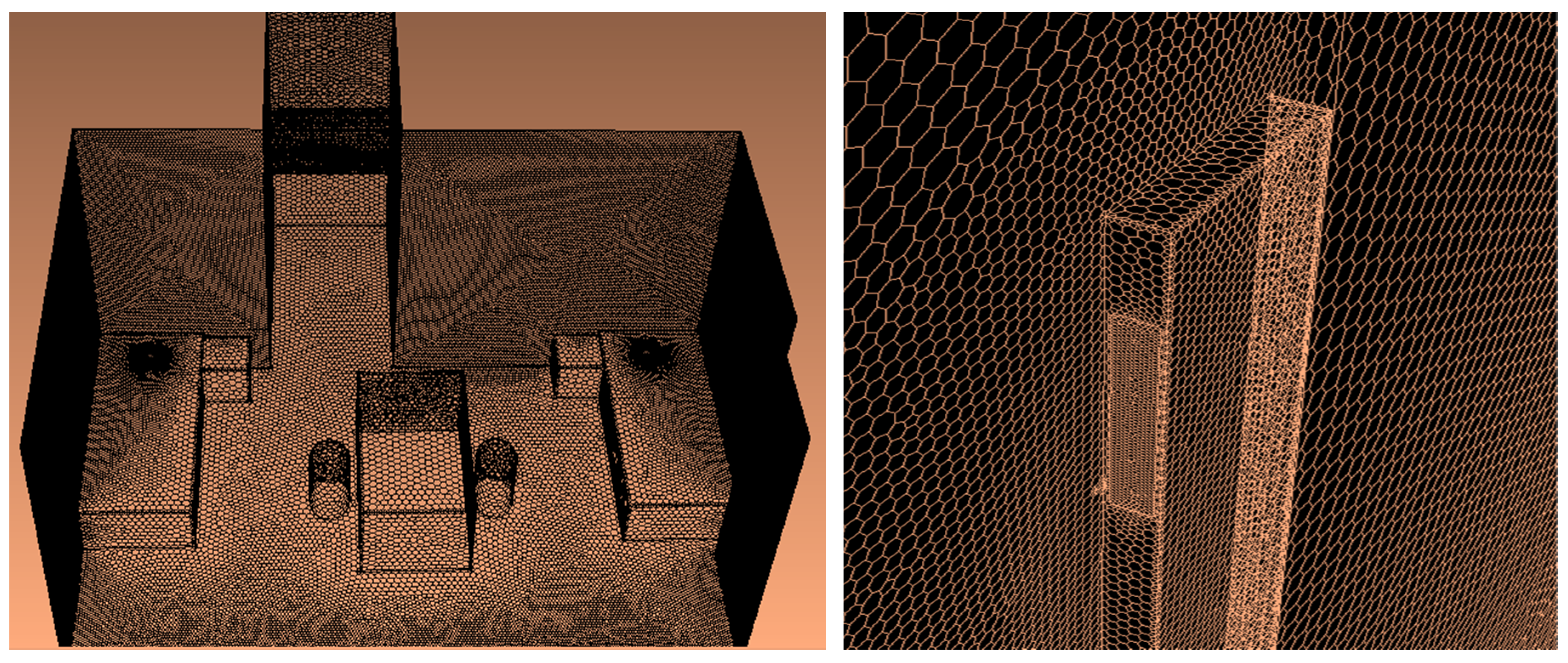
Figure 4.
Comparison of the mean indoor CO2 concentration for different air flow rates: Numerical model vs. analytical method.
Figure 4.
Comparison of the mean indoor CO2 concentration for different air flow rates: Numerical model vs. analytical method.
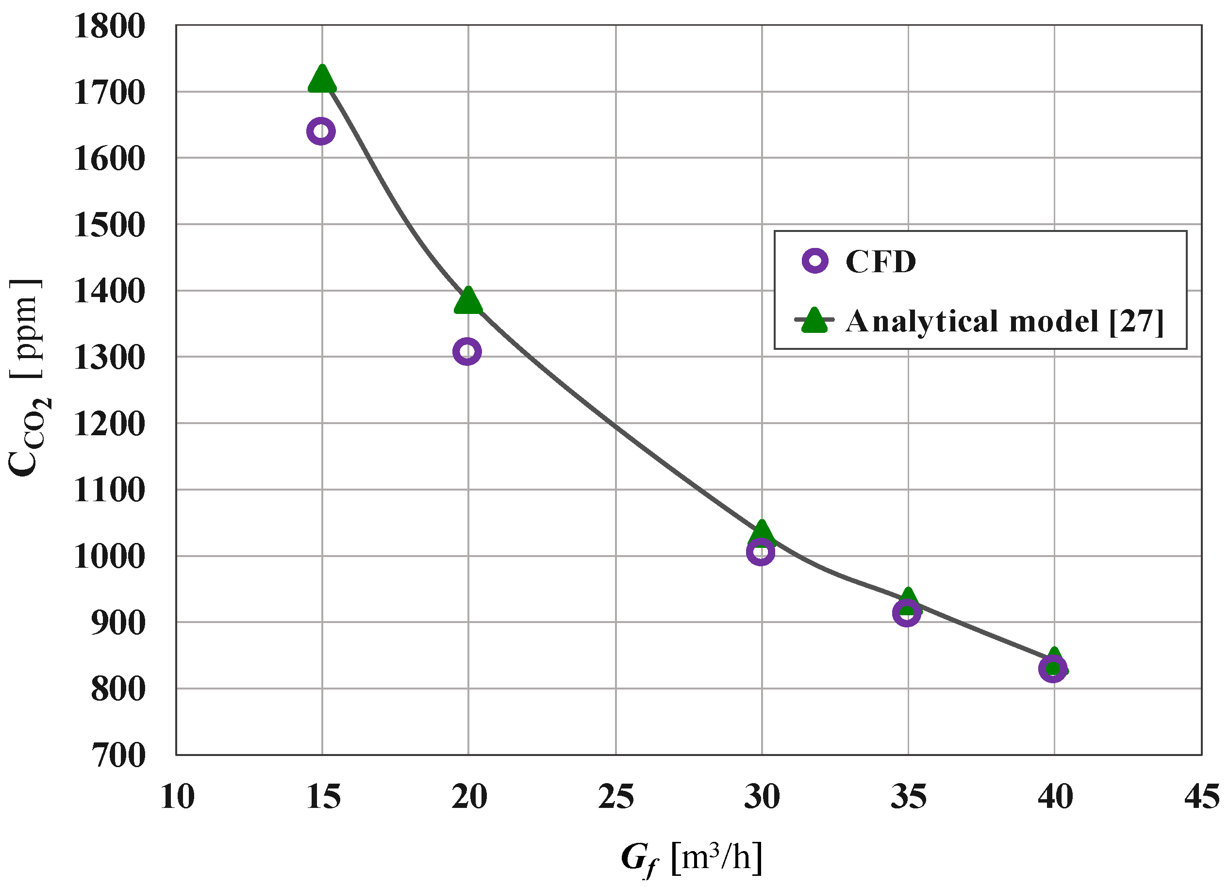
Figure 5.
Air temperature distribution on the horizontal plane at z = 1.1 m for cases 1 (left) and 5 (right).
Figure 5.
Air temperature distribution on the horizontal plane at z = 1.1 m for cases 1 (left) and 5 (right).

Figure 6.
Streamlines coloured by the velocity magnitude on the horizontal plane at z = 1.1 m for cases 1 (left) and 5 (right).
Figure 6.
Streamlines coloured by the velocity magnitude on the horizontal plane at z = 1.1 m for cases 1 (left) and 5 (right).

Figure 7.
Contours of the air temperature (left) and velocity magnitude (right) on vertical planes at y = 1 and 3 m for Case 3.
Figure 7.
Contours of the air temperature (left) and velocity magnitude (right) on vertical planes at y = 1 and 3 m for Case 3.
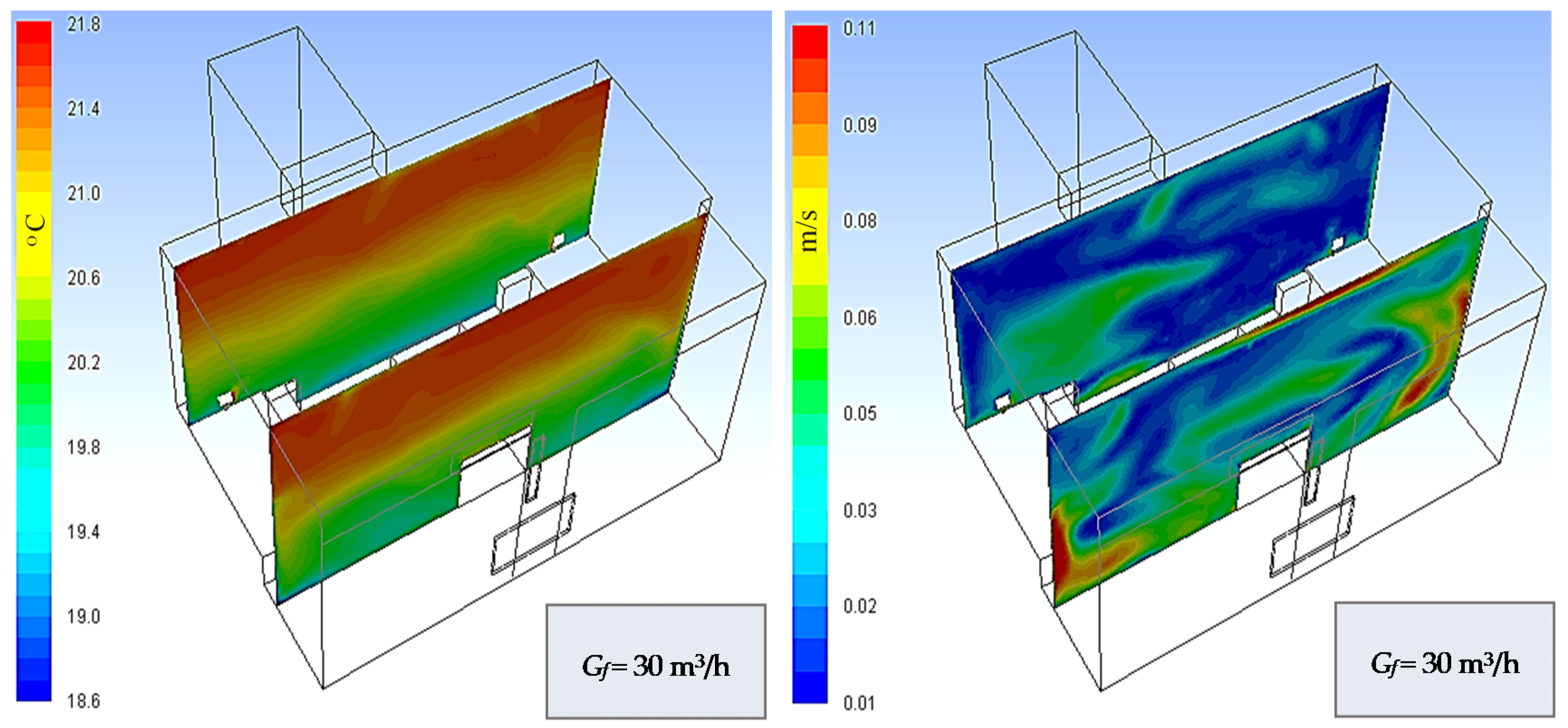
Figure 8.
Airflow field in vicinity of the HRV and radiator on the vertical plane at y = 0.1 m for the maximum air flow rate.
Figure 8.
Airflow field in vicinity of the HRV and radiator on the vertical plane at y = 0.1 m for the maximum air flow rate.

Figure 9.
Temperature distribution in vicinity of the HRV and radiator on the vertical plane at y = 0.1 m for the maximum air flow rate.
Figure 9.
Temperature distribution in vicinity of the HRV and radiator on the vertical plane at y = 0.1 m for the maximum air flow rate.

Figure 10.
Distribution of the local mean age of the air with streamlines on horizontal plane at z = 1.1 m for cases 1 (left) and 5 (right).
Figure 10.
Distribution of the local mean age of the air with streamlines on horizontal plane at z = 1.1 m for cases 1 (left) and 5 (right).
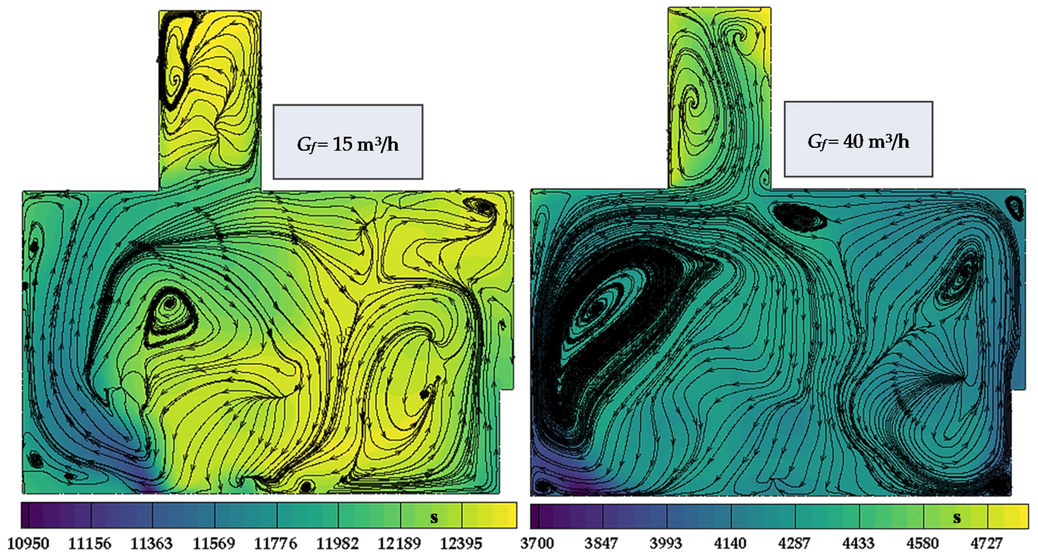
Figure 11.
Variations of the age of the air and air change efficiency (ACE) with the air flow rate.

Figure 12.
Contours of the CO2 concentration in ppm on the horizontal surface at z = 1.1 m.

Figure 13.
Distribution of the dimensionless Formaldehyde concentration at height 1.1 m.

Figure 14.
Ventilation efficiency and air change per hour (ACPH) for various air flow rates.
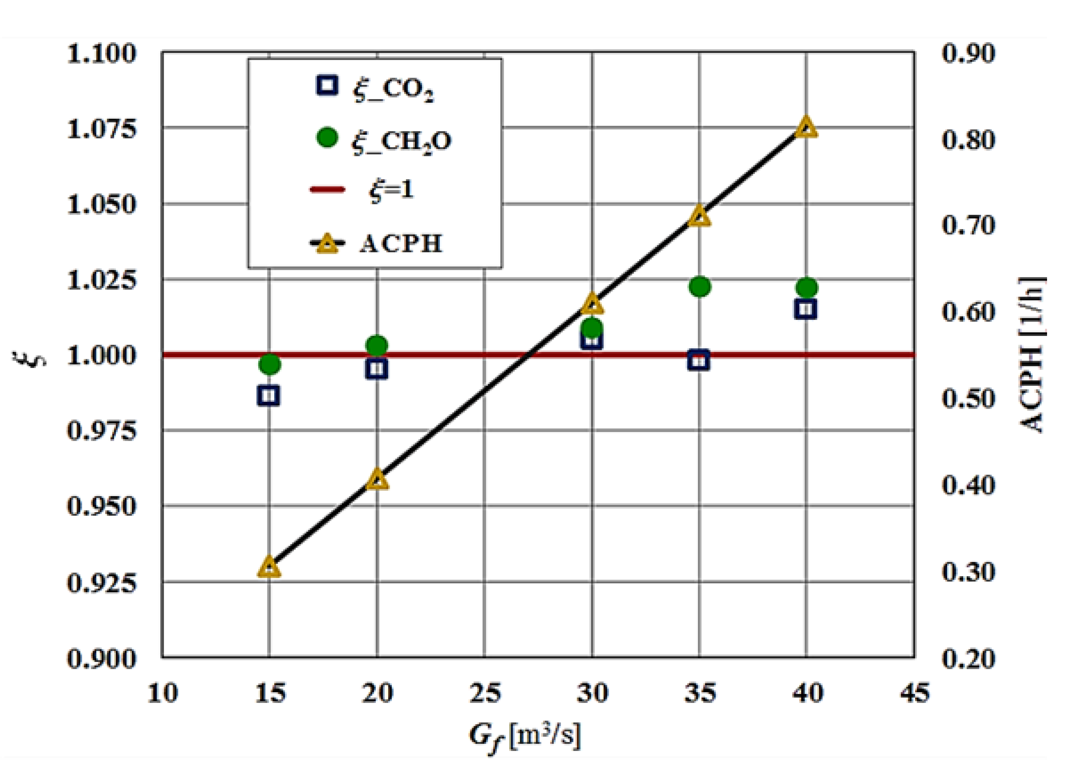
Figure 15.
Contours of the thermal comfort indices on the horizontal plane at height 1.1 m for Case 1.
Figure 15.
Contours of the thermal comfort indices on the horizontal plane at height 1.1 m for Case 1.

Figure 16.
Contours of the thermal comfort indices on the horizontal plane at height 1.1 m for Case 3.
Figure 16.
Contours of the thermal comfort indices on the horizontal plane at height 1.1 m for Case 3.
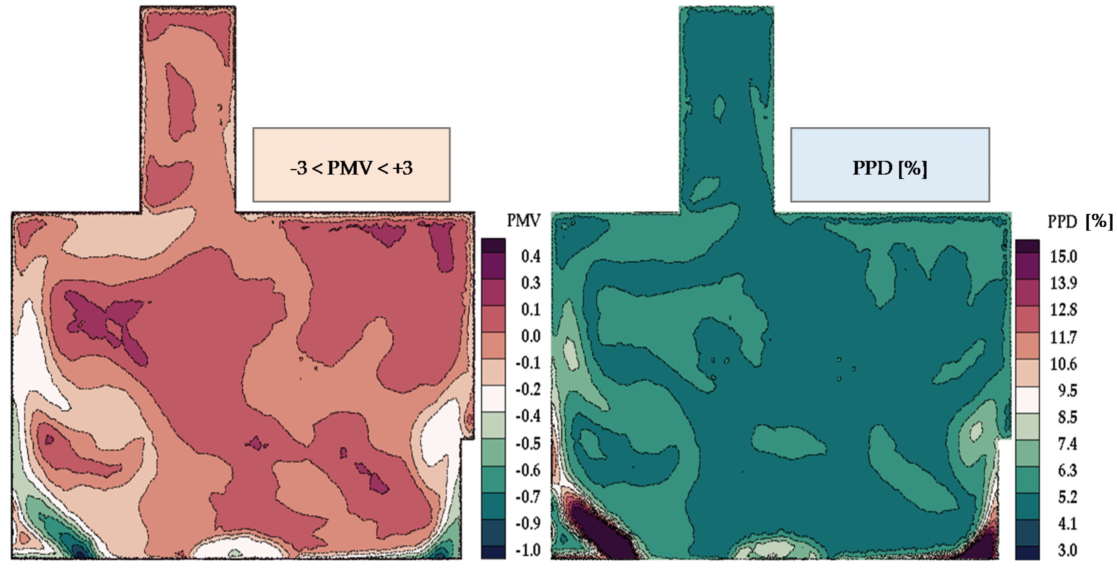
Figure 17.
Contours of the thermal comfort indices on the horizontal plane at height 1.1 m for Case 5.
Figure 17.
Contours of the thermal comfort indices on the horizontal plane at height 1.1 m for Case 5.
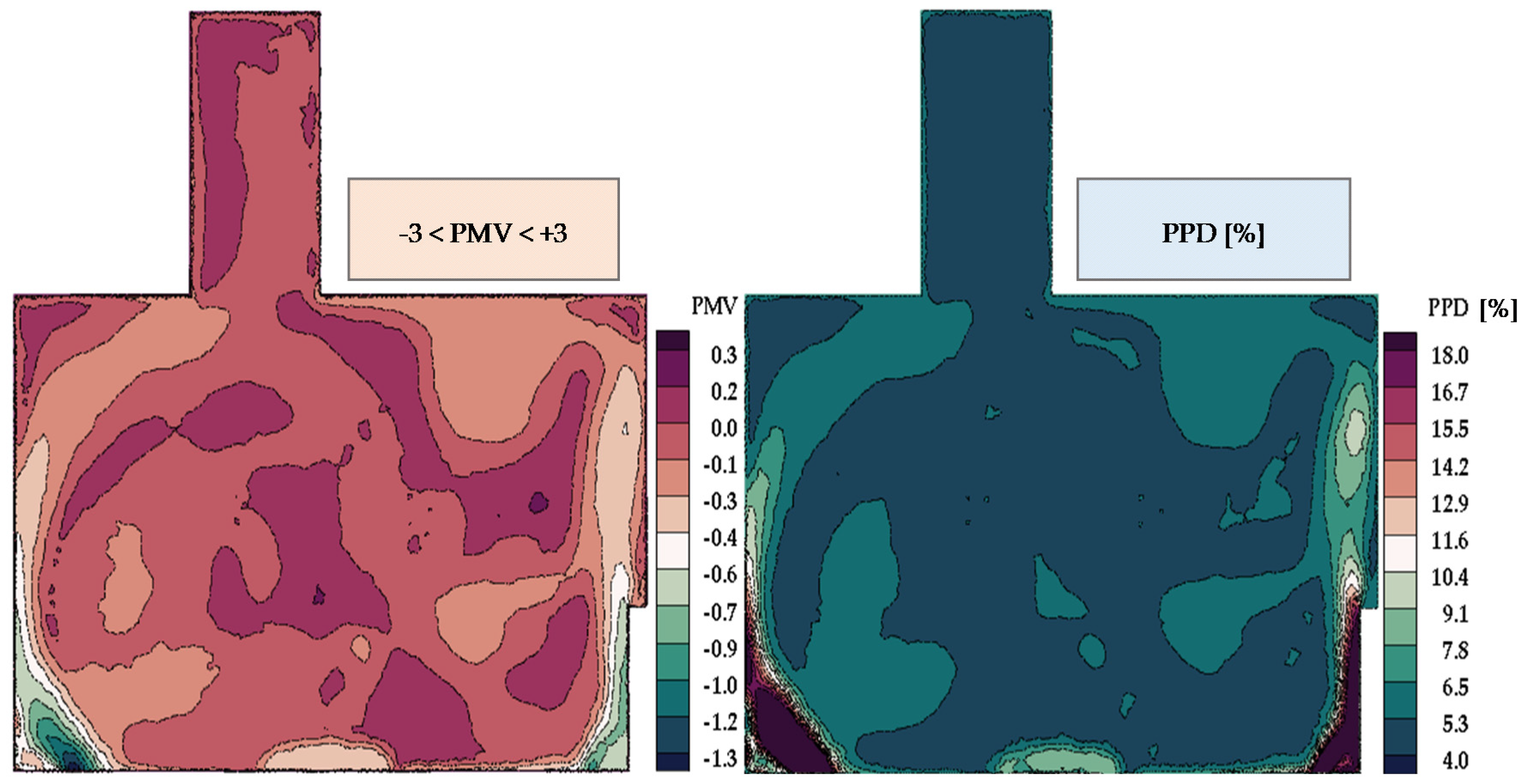
Figure 18.
Profiles of the draught rate (DR) on the horizontal surface at heights 1.1 m (left) and 1.5 m (right) for Case 5.
Figure 18.
Profiles of the draught rate (DR) on the horizontal surface at heights 1.1 m (left) and 1.5 m (right) for Case 5.

Figure 19.
Variations in the PPD with alterations in the clothing insulation for different air flow rates.
Figure 19.
Variations in the PPD with alterations in the clothing insulation for different air flow rates.


Table 1.
Details of the HRV system’s working conditions.
| Case | Air Flow Rate (Gf) [m3/h] | Mass Flow Rate [kg/s] | Air Velocity at Inlet [m/s] | Thermal Efficiency [%] |
|---|---|---|---|---|
| 1 | 15 | 0.005 | 0.80 | 82 |
| 2 | 20 | 0.007 | 1.07 | 78 |
| 3 | 30 | 0.010 | 1.61 | 74 |
| 4 | 35 | 0.012 | 1.87 | 72 |
| 5 | 40 | 0.014 | 2.19 | 69 |
Table 2.
Turbulence model’s constants.
| αk, αε | C1ε | C2ε | C*1ε | η | η0 | γ | Cμ |
|---|---|---|---|---|---|---|---|
| 1.39 | 1.42 | 1.68 | 4.377 | 0.012 | 0.0845 |
Table 3.
Mean values of the air temperature, operative temperature, velocity and turbulence intensity for various air flow rates.
Table 3.
Mean values of the air temperature, operative temperature, velocity and turbulence intensity for various air flow rates.
| Case | Gf [m3/h] | [°C] | [°C] | [m s−1] | I [%] |
|---|---|---|---|---|---|
| 1 | 15 | 20.97 | 20.64 | 0.026 | 0.92 |
| 2 | 20 | 20.91 | 20.60 | 0.029 | 0.97 |
| 3 | 30 | 20.78 | 20.51 | 0.034 | 1.06 |
| 4 | 35 | 20.69 | 20.46 | 0.037 | 1.13 |
| 5 | 40 | 20.58 | 20.36 | 0.041 | 1.22 |
Table 4.
Effect of the indoor relative humidity on thermal comfort indices.
| RH [%] | 40 | 50 | 60 | 70 | ||||||||
| Gf [m3/h] | 15 | 30 | 40 | 15 | 30 | 40 | 15 | 30 | 40 | 15 | 30 | 40 |
| PMV | −0.25 | −0.29 | −0.33 | −0.19 | −0.24 | −0.28 | −0.14 | −0.19 | −0.22 | −0.08 | −0.13 | −0.17 |
| PPD [%] | 6.27 | 6.80 | 7.25 | 5.77 | 6.20 | 6.59 | 5.39 | 5.73 | 6.03 | 5.14 | 5.37 | 5.60 |
Publisher’s Note: MDPI stays neutral with regard to jurisdictional claims in published maps and institutional affiliations. |
© 2020 by the authors. Licensee MDPI, Basel, Switzerland. This article is an open access article distributed under the terms and conditions of the Creative Commons Attribution (CC BY) license (http://creativecommons.org/licenses/by/4.0/).
Share and Cite
MDPI and ACS Style
Jahanbin, A.; Semprini, G. Numerical Study on Indoor Environmental Quality in a Room Equipped with a Combined HRV and Radiator System. Sustainability 2020, 12, 10576. https://doi.org/10.3390/su122410576
AMA Style
Jahanbin A, Semprini G. Numerical Study on Indoor Environmental Quality in a Room Equipped with a Combined HRV and Radiator System. Sustainability. 2020; 12(24):10576. https://doi.org/10.3390/su122410576
Chicago/Turabian StyleJahanbin, Aminhossein, and Giovanni Semprini. 2020. "Numerical Study on Indoor Environmental Quality in a Room Equipped with a Combined HRV and Radiator System" Sustainability 12, no. 24: 10576. https://doi.org/10.3390/su122410576
Note that from the first issue of 2016, this journal uses article numbers instead of page numbers. See further details here.