Greenhouse Gas Emissions Growth in Europe: A Comparative Analysis of Determinants

Abstract

Understanding the underlying reasons for greenhouse gas (GHG) emissions trends in different countries is fundamental for climate change mitigation. This paper identifies the main determinants that affect GHG emissions growth and assesses their impact and differences among countries in Europe. Previous studies have produced inconclusive results and presented several limitations, such as the lack of quality of the data used, the reduced identification of determinants and the use of methods that did not enable hypothesis testing. Conversely, this research identifies an extended list of determinants of GHG emissions, performs an in-depth statistical analysis and contrasts the significance of determinants using panel data and multiple linear regression models for the period 1990–2017 for the main Eurozone countries. The study found that GDP and final energy intensity are the main drivers for the reduction of GHG emissions in Europe. Furthermore, energy prices are not significant and heterogeneous results are found for the renewable energy, fuel mix and carbon intensity determinants, pointing to a different behavior at the country level. The uneven impact of the main determinants of GHG emission growth suggest that a differentiated application of European policies at country level will enhance the efficiency of mitigation efforts in Europe.

1. Introduction

According to the latest greenhouse gas (GHG) emissions inventory of the European Union (EU), the total GHG emissions (excluding Land Use and Land Use Change and Forest—LULUCF—emissions) for the 28 EU countries (EU28) decreased by 23.45% from 1990 to 2017. The EU attributes this decrease in GHG emissions to a combination of factors, such as improved energy efficiency, the growing share of renewables, the use of less intensive carbon fuels and the economic recession [1].

The main contributor to EU28 GHG emissions at the sector level in the period 1990–2017 is the energy sector, with a contribution that ranges from 77.0% in 1990 to 77.9% in 2017. The second largest contributor to EU28 GHG emissions is the agriculture sector, with a participation in national total emissions that ranged from 9.6% in 1990 to 10.2% in 2017. The third and the fourth highest emitting sectors in the EU28 were the industrial processes and product use (IPPU) and waste sectors, with contribution ranges for the period 1990–2017 of 9.2–8.7% and 4.3–3.2%, respectively. The temporal evolution of the GHG emissions for EU28 is illustrated in Figure 1.

Within the energy sector, the major GHG emitting activities for this period were the energy industries and transport, which were jointly responsible for approximately 50% of total emissions reported for 2017 (27% energy industries and 22% transport). Most emitting activities reported in [1] significantly reduced their emission levels in the inventoried period, except for transport, which increased its emissions by 19.24%.

At the country level, the change in GHG emissions in the period 1990–2017 ranged between the 57.65% decrease in Lithuania to the 58.33% increase in Cyprus. In the most developed economies in Europe, this rate also shows a wide range, including a 27.53% decrease in Germany, a 17.39% decrease in Italy, a 9.61% increase in Ireland, a 17.93% increase in Spain or a 4.56% increase in Austria. In the same period, the changes in GDP and population ranged from 21.23% to 320.72% and from −26.91% to 55.73%.

Table 1. EU28 GHG emissions growth. Percentage of change 1990–2017.

Country	% of Change 1990–2017			Country	% of Change 1990–2017
	GHG	GDP	Pop		GHG	GDP	Pop
Austria	4.56%	66.32%	14.76%	Italy	−17.39%	21.23%	6.87%
Belgium	−21.86%	59.26%	14.11%	Latvia	−56.94%	131.91%	−26.91%
Bulgaria	−39.75%	66.20%	−19.00%	Lithuania	−57.65%	146.57%	−22.90%
Croatia	−21.31%	66.20	−12.96%	Luxemburg	−19.76%	163.34%	55.73%
Cyprus	58.33%	71.38	49.27%	Malta	0.00%	80.37%	30.61%
Czech Republic	−34.81%	66.78%	2.09%	Netherlands	−12.47%	73.04%	14.70%
Denmark	−30.19%	56.89	11.94%	Poland	−12.75%	165.13%	−0.17%
Estonia	−48.36%	148.23%	−16.23%	Portugal	19.56%	43.43%	3.14%
Finland	−22.21%	56.75%	10.63%	Romania	−54.14%	94.14%	−15.37%
France	−14.52%	51.77%	2.52%	Slovakia	−40.96%	51.77%	2.79%
Germany	−27.53%	51.20%	31.66%	Slovenia	−6.36%	71.56%	3.48%
Greece	−7.45%	25.44%	6.40%	Spain	17.93%	72.91%	19.75%
Hungary	−31.89%	67.23%	−5.56%	Sweden	−26.15%	77.09%	17.22%
Ireland	9.61%	320.72%	36.42%	United Kingdom	−39.40%	72.44%	15.20%

Source: GHG emissions [2], GDP [3], Population [4].

shows the change in GHG emissions, GDP and population for EU28 countries.

The differences between countries in the GHG emissions change for the period 1990–2017 are explained by the diverse economic, demographic, climatic, and behavioral characteristics of each country, which involve different drivers for GHG emissions growth [5].

The understanding of both the main factors determining GHG emissions growth and the differences in the impact of these factors at country level are of the utmost importance for enhancing the design and implementation of nationally appropriate mitigation actions to reduce, as effectively as possible, GHG emissions worldwide [6,7]. The recently signed Paris Agreement will require additional and cost-effective mitigation efforts by its signatories to achieve its objective of limiting global warming to well below 2 °C and pursuing efforts to limit it to 1.5 °C [6].

The factors effecting the GHG emissions trend and the differences between countries have been analyzed broadly. A large part of the research uses decomposition analysis, a statistical technique in which the economy is broken down into predetermined factors of interest for analyzing the impact of each of them on GHG emissions growth. However, decomposition analysis does not allow for hypothesis testing, impeding the ability to obtain reliable empirically tested conclusions. Relevant examples of this type of studies are [8,9,10,11,12,13,14].

The authors in [15,16,17] improved the decomposition analysis using regression techniques for assessing the inequality of GHG emissions and emission intensity. These analyses, however, did not aim at analyzing the reasons for the GHG emissions growth, and contained a limited identification and assessment of determinants of GHG emissions. The limited identification of determinants is also found in other studies, such as [18,19,20,21].

Other deficiencies found in the research of determinants of GHG emissions are the non-inclusion of variables with high explanatory power in stochastic models (such as fuel mix, the structure of the economy or the fleet of vehicles), the use of own estimations and heterogeneous data sources (as [21]); multicollinearity among variables (as in [19,20,22]) and non-stationary data series (as [23,24,25]).

The objective of this paper is to overcome the limitations found in previous studies to identify the main determinants that affect national GHG emissions growth and assess their impact and differences among countries in Europe. For this, we use a panel data model on a consistent dataset (which includes data from Eurostat, OCDE and the United Nations Framework Convention on Climate change (UNFCCC)) for the years 1990–2017 on the main Eurozone countries. We identify an extended list of determinants of GHG emissions, assessing the compatibility of the variables selected through an in-depth statistical analysis and contrasting the significance of each determinant for explaining GHG emissions growth. Furthermore, we explore whether there are significant differences between countries regarding the impact of each determinant in the GHG emission growth.

Extended Literature Review and Hypothesis Development

In previous research, the studies on determinants of GHG emissions growth are categorized within three methodological categories: Kaya identity, IPAT identity and decomposition analysis. [18,23] provide an exhaustive bibliography review of the studies encompassed in each of these categories and have therefore not been reproduced in this study.

As pointed out by [25], most of the research included in these three categories presented two main limitations: (i) they do not allow hypothesis testing and (ii) they assume that the functional relationships between factors are proportional. These limitations are a consequence of the statistical methods used in the empirical research. Studies suffering from these limitations are not included in this paper.

The following paragraphs provide a description of the most relevant studies found in the bibliography relevant to the objectives of this study—the identification of determinants of GHG emission growth, the assessment of their impact and the analysis of differences between countries.

Among the most recent empirical research, [23] is the most exhaustive identification of GHG emission determinants found in the literature, with nine determinants of GHG emissions growth being identified and analyzed. The authors in [23] concluded that energy prices are the main variable explaining differences in GHG emissions among countries. Several areas of improvement were identified in the study: (i) from an extended list of potential determinants identified, only three factors are selected as predictors for explaining differences between countries—energy prices, economic output per capita and environmental governance; (ii) the trend is not considered in the analysis and, (iii) the list of determinants identified, even it is a good approximation, could be enhanced.

The authors in [24] analyzed the impact on GHG emissions of GDP per capita, population, renewable energy, energy intensity and the economic crisis in Spain for years 2000–2011, finding that GDP per capita and the penetration of renewable energy sources are the main drivers of GHG emissions growth. The coefficient of determination (R2) obtained in [24] ranged from 0.96 to 0.99, depending on the specification of the model. However, the variables used could be non-stationary, as a unit root test of the sample was not reported. The results of this study are therefore questionable.

The authors in [19] evaluated the impact of economic growth, energy consumption and renewable energy sources on GHG emissions using fixed and random effect panel regression models to analyze data from the 28 EU member states from 1990 to 2012. This study found that GDP and primary energy consumption are the main variables affecting GHG emissions growth. However, while the methodology used was more consistent than previous approaches, the scarcity of variables considered in the analysis was the main limitation of this study. Following a similar approach, the authors in [20] analyzed the impact of economic growth, energy consumption, energy taxes and research and development during 1995–2014 for 22 EU countries, using a fixed effect panel data. This study carried out an extensive literature review of studies based on panel-data regression models addressing the relationship between GDP (or economic growth), GHG emissions and energy consumption. The results of the model reach a R2 of 0.9577, with all the variables tested being significant for explaining the evolution of GHG emissions.

The authors of [22] analyzed CO₂ emission growth in China using panel data econometric models for the years 1995–2012. The variables tested in this study were GDP per capita, industry share of GDP, population, energy consumption and a set of qualitative variables (policy, government effectiveness and location). This study concluded that economic growth and the industry’s share of GDP are the key drivers of CO₂ emissions. In view of the scope of our study, the limitations of [22] were related to the gases considered (only CO₂ instead of all greenhouse gases accounted by [26]) and the different geographical scope.

The authors in [21] analyzed the trend of changes in GHG emissions in ten countries over 40 years (1971–2012) using multiple linear regression model based on the Kaya identity. This study found that different factors are critical for explaining GHG emission evolution in different countries (carbon intensity for China, GDP for US, Canada and India, etc.). However, the GHG emissions data used in this study were a combination of heterogeneous data sources and own estimations, making the data used for different countries not comparable and the results questionable.

The authors in [25] studied the driving factors of GHG emissions in the EU28 during the period 1990–2014, focusing in the transport sector, one of the key contributors to national total GHG emissions [27]. Using panel data techniques, this study concluded that population, real GPD per capita, transport volume, transport energy intensity, and changes in modal share and in energy source mix are the main drivers of greenhouse gas emissions in the EU transport sector. Nevertheless, the scope of the study was not national total GHG emissions, and therefore the results need to be taken into account with caution.

Aiming at improving the identification of the determinants of GHG emissions, National Inventory Reports submitted to the United Nations Framework Convention of Climate Change (UNFCCC) in 2019 by the countries within the scope of the research have been analyzed [2]; this analysis was mainly focused on the energy and Industrial processes and Product use sectors, responsible for more than 80% of emissions in all European countries [27]. As we expected, not all countries identified the same determinants for the GHG emission evolution by emission source. Nevertheless, energy efficiency, production levels (GDP), renewable energy sources, energy efficiency, the fuel mix (substitution of fuels with high carbon contents), and technology factors were identified as key determinants in most countries’ reports.

Given the scope of the research, the identification of determinants performed in this bibliography review relies on the previous recognition of factors by other studies, which in turn depends on (i) the relative importance of these factors to explain national total GHG emissions; and (ii) the availability of data. The determinants not fulfilling these two criteria fall outside the scope of this exercise. Nevertheless, there might be potential determinants which are either not previously identified in the bibliography or are not quantitative in nature that might be of interest for explaining the evolution of GHG emissions. This is the case for circular economy practices and ecosystem valuation [28].

In short,

Table 2. Summary of determinants identified in the more relevant studies found in the bibliography review.

Study	Factors Affecting GHG Emission Growth
[1]	Fuel mix, energy efficiency, renewables, structural changes in the economy, temperature, production levels (GDP), emission reduction measures, carbon intensity, switch from gasoline to diesel and use of biofuels
[19]	Economic growth, energy consumption and renewable energy sources
[20]	Economic growth, energy consumption, energy taxes and research and development.
[21]	Carbon intensity, GDP, energy intensity, population.
[22]	GDP per capita, industry sector, population, energy consumption, among a set of qualitative variables (policy, government effectiveness and location).
[23]	Climate, population pressure, economic output, technological development, industrial structure, energy prices, environmental governance, environmental expenditure and environmental pricing.
[24]	GDP per capita, population, renewable energy, energy intensity and the economic crisis (dummy).
[25]	Population, economic activity, transport volume, transport energy intensity and transport activity composition in terms of modal share and of energy source mix.
[29]	Higher technical efficiencies due to the closure of plants (replacement of old lignite plants), increasing use of renewable and nuclear, electricity demand, production evolution (petroleum refining), production level (GDP), emission reduction measures, refueling in other countries (fuel prices), substitution of diesel fuel for gasoline, use of ad-mixtures with biodiesel, fuel changeovers (fuel mix), higher energy and technical efficiencies and temperature.
[30]	Contribution of renewable energy sources, substitution of solid and liquid fuels by natural gas and biomass, improvements in energy efficiency, abatement technologies, GDP (production levels), km driven, fuel prices, introduction of alternative vehicles in the fleet, shift in the fuel mix, temperature, modernization of heating systems.
[31]	Closure of six coke plants, GDP, technological improvements, increase of the number of combined heat-power installations and the switch from solid fuels (coal) to gaseous fuels (natural gas) and renewable fuels, energy efficiency (“rational energy use”), technological improvements, evolution of GDP (economic context), abatement technologies, number of vehicles, vehicles km, switch from petrol to diesel cars, population (number of dwellings), temperature (degree days), number of employees in the commercial and institutional sector, switch from liquid fuels to gaseous fuels, for F-gases: The growing consumption of HFC is directly linked to the implementation of the Montreal Protocol and EU Regulation 2037/2000.
[32]	GDP, changes in the fuel mix in the production of electricity in thermic plants, national carbon policies, renewable policies, production levels (GDP), fuel mix evolution, number of vehicles, vehicles km, temperature, income, from 2013: impact of national law for fluorinated gases.
[33]	Precipitation, electricity imports, renewable energy production, temperature, increased shares of forest-based fuels, high energy intensity, technical abatement measures, long distances, km driven (vehicles km), transition, from gasoline to diesel cars, growing share of biofuels used in road transport and improving fuel efficiency of vehicles (from 2010), substitution of ozone depleting substances (ODS) by F gases, changeover from oil heating to district or electric heating (this is not a proxy, but a change in the allocation of emissions).
[34]	As the country relies on the production of electricity using nuclear energy, the main contributor to emissions is the transport sector, total vehicles fleet, fuel changeovers (solid fuels decrease, natural gas increase), temperature, precipitation, import-export of electricity, fuel changeovers (solid fuels decrease, natural gas increase), several refineries have been closed, production levels (GDP), technological efficiency, carbon and energy efficiency, abatement technologies, vehicles fleet, biofuels (from 2005), increased fuel efficiency of new vehicles, fuel prices, limited speed and fuel efficiency of new cars.
[35]	Temperature, import-exports of electricity, fuel mix, temperature, contribution of nuclear and renewable, import-exports of electricity, production levels (GDP), road transport volumes, introduction of biofuels (2003), refilling in other countries (fuel prices), fuel efficiency and diesel fleet.
[36]	GDP, fuel mix, changes in the fuel mix (displacement of oil by natural gas), energy efficiency, GDP, share of renewables in gross electricity consumption, wind and hydro electricity generation (precipitation and wind), production levels (GDP), fuel mix (large increases in use of petroleum coke), closure of high energy intensity production plants, road transport volumes (vh kn, passengers fleet and goods vehicles), fuel tourism (fuel price), impact of registration tax and road tax introduced in 2008, biofuels obligation scheme and population.
[37]	Fuel mix, GDP, European policies (ETS and renewables), substitution of fuels with high carbon contents by methane gas in the production of electric energy and in industry, increase in the use of renewable sources, Production (GDP), efficiency (particularly in the chemical sector), abatement technology, vehicle fleet, vehicles km, technology development and switch from gasoline to diesel
[38]	GDP, energy demand, mobility, investment in renewable sources, energy efficiency, precipitation, GDP, energy demand, production levels (GDP), vehicle fleet, income and investment in road infrastructure

summarizes the determinants of GHG emissions identified by sources in our bibliography review. The wording used in each research has been maintained as far as possible, aiming at illustrating the variability of determinants and variables used in each research.

The bibliography review shows that both academic studies and the reports submitted by countries to the UNFCCC identify a wide set of variables that affect GHG emission growth, and the results of the studies analyzed led to different and inconclusive results. Thus, the hypotheses to be tested in this empirical study are:

• What are the key explanatory factors of GHG emissions growth within the EU (H1)?
• Is the weight of each explanatory factor for GHG emissions growth different for each EU country (H2)?

2. Materials and Methods

We followed the methodological steps illustrated in Figure 2. First, we carried out an exhaustive bibliography review for identifying the determinants of GHG emissions. Based on this review, we selected a set of variables for making a preliminary analysis of the data to avoid multicollinearity and non-stationarity problems, among others.

Next, we designed a regression model for explaining the temporal evolution of national total GHG emissions. As this model is fitted at a national level, we also estimated a panel data model for all countries to test if the weights of the explanatory factors for each country are equal to those of the EU as a whole.

2.1. Determinants of GHG Emissions: Definition of Variables

To select the explanatory factors, we considered: (i) high hypothetical correlation with national total GHG emissions; and (ii) statistical significance in previous studies.

The explanatory variables that we initially selected along their causal theory, supporting literature and relation expected sign are summarized in

Table 3. Causal relationship for each determinant of GHG emissions.

Variable	Causal Relationship	Relation Expected Sign	Empirical Studies
Population [Pop]	Increased population leads to higher levels of consumption and production, which would produce higher GHG emissions.	(+)	[21,23,24,29,36];
Gross Domestic Product [GDP]	For producing GDP, there is a need to consume products (fuel, feedstock, food, etc.) and carry out processes (industrial, agricultural, etc.) that produce GHG emissions. Higher levels of GDP would involve higher GHG emissions.	(+)	[19,21,24,29,30,31,32,33,34,35,36,37,38]
Temperature—Heating degree days [HDD]	The use of heating systems produces GHG emissions. Colder temperatures imply more intensive use of heating systems and higher level of GHG emissions.	(+)	[1,23,29,30,31,33,34,35]
Temperature—Cooling degree days [CDD]	The use of air conditioning produces GHG emissions due to the use of fluorinated gases in these systems. Warmer temperatures would imply more intensive use of air conditioning and a higher level of GHG emissions.	(+)
Primary energy consumption [PEC]	The consumption of fuels produces GHG emissions. Primary energy consumption measures the total energy demand of a country. It covers consumption of the energy sector itself, losses during transformation (for example, from oil or gas into electricity) and distribution of energy, and the final consumption by end users.	(+)	[18,20,22,29,30,31,32,33,34,35,36,37,38]
Final Energy consumption [FEC]	Final energy consumption is the total energy consumed by end users, such as households, industry and agriculture. It is the energy which reaches the final consumer’s door and excludes that which is used by the energy sector itself.	(+)	[19,20,22,29,30,31,32,33,34,35,36,37,38]
Primary and Final energy intensity [PEI] and [FEI]	Energy intensity represents the amount of energy needed for generating a unit of GDP. Higher levels of energy intensity lead to increased GHG emission levels.	(+)	[1,18,20,24,33,36,38]
Fuel prices [FP]	Higher prices lead to lower energy consumption levels. The variable used is estimated as an weighted average of different fuel prices (see below a more detailed explanation of the variable used)	(−)	[1,23,36];
Carbon intensity [CI]	Amount of GHG emissions by unit of energy consumed. Lower levels of carbon intensity occur because of the use of low carbon fuels and technology efficiency. Higher levels of CI would involve higher GHG emissions.	(+)	[18,21,36]
Renewable energy [RES]	The use of renewable sources instead of other fossil intensive alternatives avoids or reduce GHG emissions. This variable consists in the share of RES in total gross inland consumption.	(−)	[18,19,23,24]
Structure of the economy [SE]	There are certain economic activities which are more resource-intensive, producing higher GHG emissions. This variable is calculated as the gross added value of the manufacturing industries split by national total gross added value.	(+)	[1,29];
Fuel mix [FM]	There are fuels which produce more GHG emissions than others due to a higher carbon content. Solid fuels have higher carbon content than liquid and gas fuels. This variable is calculated as the solid fuel gross inland consumption split by total gross inland consumption.	(+)	[1,16,29,30,32,35,36,37]
Fleet [Fleet]	Motor vehicles used for transportation purposes consume fuels which produce GHG emissions.	(+)	[25,29,30,31,32,33,34,35,36,37,38,39,40]

.

2.2. Models

We used two models for empirical testing: a linear panel data model and a multiple linear regression model for each country. The first model was used for assessing if the determinants selected were significant for explaining GHG emission growth in the EU (H1). The second model was used to assess the differences in impact of each determinant (H2).

The following expression is the linear panel data model used:

$$y_{i,t}={{\displaystyle \sum }}_{k=1}^K{\beta }_k·x_{i,k,t}+u_{i,t}$$

(1)

where y is the GHG emissions of country i (i = 1,…,N) for year t (t = 1,…,T); x is a k regressor (k = 1,…,K) or potential explanatory factor.

There were two possible estimates of Expression (1) according to the term u. If we considered constant individual and idiosyncratic effects for each country, then we obtained a fixed effect panel data model, where $u_{i,t}={\beta }_{0,i}+{\epsilon }_{i,t}$, and ${\epsilon }_{i,t}~i.i.d.\left(0, {\sigma }^2\right)$. For this case, the parameter estimation was made by ordinary least squares (OLS) including news regressors, i.e., a dummy for each country.

The second estimation supposed that $u_{i,t}={\beta }_0+{\gamma }_{i,t}+{\epsilon }_{i,t}$, ${\gamma }_{i,t}~i.i.d.\left(0, {\sigma }_i^2\right)$ and ${\epsilon }_{i,t}~i.i.d.\left(0, {\sigma }^2\right)$, resulting in a random effect panel data model. For this case, the parameter estimation was made by the generalized least squares (GLS) method, which provided a robust estimation. This method is a variant of OLS but ponders the estimation from within and between estimators.

Selecting fixed or random effects depends on the relationship among the fixed effects and regressors, and this selection was made using the Hausman test. The null-hypothesis of this test is that correlation among individuals effects and regressors is zero; if the null-hypothesis is not rejected, a fixed effects panel data model is used; otherwise, a random effects panel data model is selected (for the detailed advantages and disadvantages of each model, see [19]).

Once the panel data parameters were selected, the first hypothesis of the study (H1) was tested as $\forall k {\beta }_k\ne 0$.

The second model used in this study was the following multiple linear regression model for each country i:

$$y_t={\alpha }_0+{{\displaystyle \sum }}_{k=1}^K{\alpha }_k·x_{k,t}+e_t$$

(2)

Using this expression, the second hypothesis (H2) was tested as follows:

• Country i showed the same weights as the EU for all explanatory factors of GHG emissions (H2a): $\forall k {\beta }_k-{\alpha }_k=0$. This test was distributed as Chi-square distribution with k freedom degree (Wald test).
• Country i showed the same weights as the EU for each k-explanatory factor of GHG emissions (H2b): ${\beta }_k-{\alpha }_k=0$. This test was distributed as Chi-square distribution with one freedom degree (Wald test).

2.3. Data

This empirical research focused on the Eurozone to avoid distortions in the data due to currency exchange rates. Our sample contained countries with aggregated GDP at 95% of total GDP of the Eurozone: Germany, Austria, Belgium, Spain, Finland, France, Netherlands, Ireland, Italy and Portugal.

For GHG emissions, we used the data from national GHG emission inventories submitted to the United Nations Convention of Climate Change [2]. Specifically, we used national total GHG emissions without land use, land use change and forestry, extracted from the Common Reporting Framework (CRF) Table 10S1.

By using this data, we ensured that GHG emissions were calculated following specific quality standards—a common methodological framework, 2006 IPCC Guidelines [26], and annual audits [41].

The data used for the variables or potential regressors are available in Eurostat [4]. This source was prioritized as a source of information for ensuring the comparability of the data except for GDP, which was extracted from the OCDE [3], as data before 1995 was not available for all countries in Eurostat.

Generally, the variables used in this research were directly extracted from the data sources, with the exception of fuel prices. For this variable, no data were available from official sources measuring the overall price of energy at national level. Alternatively, Eurostat provides data on the prices of diesel and gasoline in [4] and data on prices for electricity and natural gas in [42]. The data for electricity and natural gas were provided for households and industrial consumers. Therefore, to obtain the variable fuel price used in this study, we calculated an average price for each commodity, pondering the level of energy consumption (industrial vs. household). Then, the prices of diesel, gasoline, electricity and natural gas were weighted by the total contribution of each source to the total final energy consumption of each country. The expression used for calculating fuel prices was the following:

$$F{P}_{t,i}^{*}={{\displaystyle \sum }}_{f=1}^{f}F{P}_{f,t,i}·\frac{E{C}_{f,t,i}}{TNE{C}_{t,i}}$$

(3)

where f is fuel type, t is year, i is an index of country, FP* is the average fuel price, FP is fuel price, EC shows the energy consumption and TNEC is the total national energy consumption. Expression (3) is a similar approach to the one followed in [23].

Using the aforementioned data sources, we obtained 14 potential regressors (see Table 3) and one dependent variable (GHG emissions).

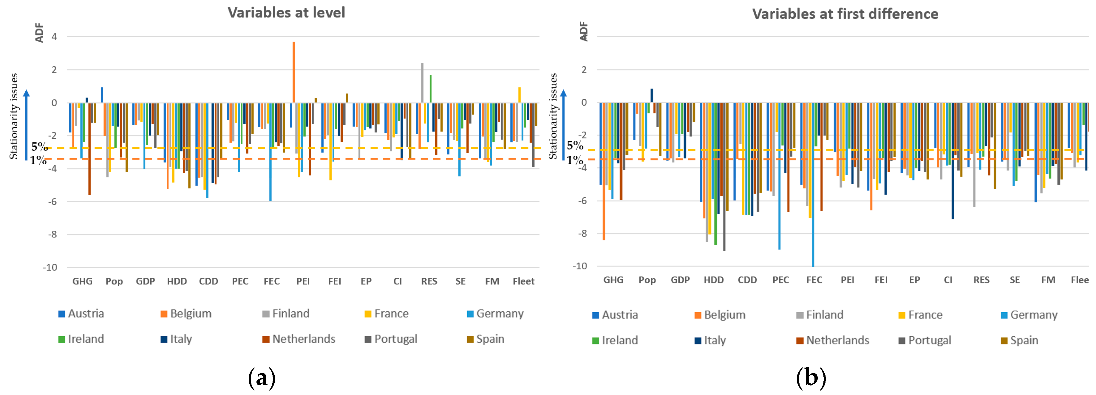
Firstly, to avoid drawbacks using non-stationary variables, we estimated the Augmented Dickey–Fuller test (ADF) on level-variable and first difference of the log-variable. Figure 3 shows the results obtained.

In Figure 3, we observe that all variables (except HDD and CDD) show stationary issues at levels. This issue was solved by taking the first difference of the natural logarithms. It must be noted that, even at the first difference, the variables population and fleet had a unit root for any country.

Next, to address another potential problem identified in the literature—the multicollinearity of the regressors—we analyzed the correlation between variables.

Table 4. Correlation matrix.

		GDP	Pop	HDD	PEC	FEC	PEI	FEI	RES	FP	SE	FM	CI	CDD	Fleet
GDP	Min	1	0.01	0.06	0.04	0.07	0.01	0.19	0.01	0.05	0.10	0.00	0.02	0.00	0.00
	Q1	1	0.12	0.12	0.22	0.15	0.15	0.25	0.11	0.25	0.29	0.03	0.08	0.02	0.05
	Q2	1	0.16	0.20	0.33	0.36	0.27	0.31	0.18	0.47	0.55	0.25	0.13	0.07	0.27
	Q3	1	0.25	0.24	0.57	0.54	0.34	0.38	0.34	0.55	0.64	0.44	0.18	0.24	0.39
	Max	1	0.54	0.32	0.74	0.84	0.72	0.61	0.51	0.59	0.83	0.48	0.38	0.36	0.75
Pop	Min	0.01	1	0.00	0.03	0.04	0.01	0.01	0.02	0.01	0.11	0.00	0.09	0.00	0.00
	Q1	0.12	1	0.03	0.07	0.12	0.04	0.12	0.13	0.08	0.18	0.10	0.16	0.03	0.16
	Q2	0.16	1	0.10	0.26	0.26	0.13	0.21	0.23	0.15	0.21	0.15	0.20	0.09	0.19
	Q3	0.25	1	0.21	0.31	0.37	0.25	0.33	0.29	0.27	0.38	0.19	0.30	0.16	0.34
	Max	0.54	1	0.40	0.54	0.54	0.48	0.43	0.45	0.46	0.58	0.36	0.50	0.25	0.45
HDD	Min	0.06	0.00	1	0.06	0.08	0.05	0.09	0.01	0.02	0.04	0.01	0.05	0.00	0.00
	Q1	0.12	0.03	1	0.33	0.33	0.30	0.46	0.06	0.06	0.06	0.11	0.17	0.04	0.03
	Q2	0.20	0.10	1	0.60	0.68	0.77	0.85	0.15	0.14	0.14	0.23	0.23	0.15	0.11
	Q3	0.24	0.21	1	0.73	0.81	0.83	0.87	0.29	0.24	0.16	0.27	0.31	0.23	0.21
	Max	0.32	0.40	1	0.87	0.88	0.90	0.93	0.57	0.39	0.26	0.50	0.51	0.33	0.37
PEC	Min	0.04	0.03	0.06	1	0.71	0.13	0.12	0.01	0.01	0.05	0.01	0.04	0.00	0.00
	Q1	0.22	0.07	0.33	1	0.83	0.75	0.56	0.35	0.05	0.16	0.14	0.22	0.02	0.11
	Q2	0.33	0.26	0.60	1	0.86	0.78	0.64	0.48	0.11	0.23	0.29	0.38	0.07	0.20
	Q3	0.57	0.31	0.73	1	0.95	0.85	0.78	0.59	0.23	0.28	0.37	0.52	0.12	0.48
	Max	0.74	0.54	0.87	1	0.98	0.94	0.83	0.63	0.42	0.37	0.66	0.63	0.40	0.65
FEC	Min	0.07	0.04	0.08	0.71	1	0.04	0.34	0.03	0.03	0.00	0.02	0.03	0.00	0.00
	Q1	0.15	0.12	0.33	0.83	1	0.45	0.71	0.24	0.08	0.14	0.22	0.11	0.01	0.11
	Q2	0.36	0.26	0.68	0.86	1	0.77	0.79	0.30	0.15	0.20	0.33	0.14	0.06	0.20
	Q3	0.54	0.37	0.81	0.95	1	0.79	0.86	0.36	0.22	0.29	0.39	0.31	0.18	0.47
	Max	0.84	0.54	0.88	0.98	1	0.86	0.94	0.57	0.32	0.53	0.43	0.53	0.44	0.65
PEI	Min	0.01	0.01	0.05	0.13	0.04	1	0.45	0.01	0.00	0.02	0.07	0.06	0.00	0.00
	Q1	0.15	0.04	0.30	0.75	0.45	1	0.84	0.20	0.11	0.12	0.13	0.18	0.13	0.08
	Q2	0.27	0.13	0.77	0.78	0.77	1	0.86	0.43	0.21	0.19	0.32	0.35	0.18	0.18
	Q3	0.34	0.25	0.83	0.85	0.79	1	0.94	0.56	0.30	0.24	0.39	0.54	0.23	0.23
	Max	0.72	0.48	0.90	0.94	0.86	1	0.97	0.65	0.48	0.62	0.67	0.71	0.51	0.32
FEI	Min	0.19	0.01	0.09	0.12	0.34	0.45	1	0.00	0.01	0.00	0.00	0.03	0.00	0.00
	Q1	0.25	0.12	0.46	0.56	0.71	0.84	1	0.15	0.08	0.17	0.14	0.13	0.04	0.10
	Q2	0.31	0.21	0.85	0.64	0.79	0.86	1	0.20	0.31	0.21	0.22	0.17	0.21	0.19
	Q3	0.38	0.33	0.87	0.78	0.86	0.94	1	0.43	0.40	0.23	0.34	0.40	0.31	0.23
	Max	0.61	0.43	0.93	0.83	0.94	0.97	1	0.52	0.54	0.77	0.47	0.58	0.44	0.32
RES	Min	0.01	0.02	0.01	0.01	0.03	0.01	0.00	1	0.04	0.02	0.07	0.04	0.00	0.00
	Q1	0.11	0.13	0.06	0.35	0.24	0.20	0.15	1	0.06	0.10	0.24	0.16	0.06	0.07
	Q2	0.18	0.23	0.15	0.48	0.30	0.43	0.20	1	0.12	0.23	0.34	0.37	0.16	0.12
	Q3	0.34	0.29	0.29	0.59	0.36	0.56	0.43	1	0.22	0.31	0.46	0.49	0.20	0.16
	Max	0.51	0.45	0.57	0.63	0.57	0.65	0.52	1	0.36	0.43	0.55	0.77	0.32	0.46
FP	Min	0.05	0.01	0.02	0.01	0.03	0.00	0.01	0.04	1	0.01	0.01	0.06	0.00	0.00
	Q1	0.25	0.08	0.06	0.05	0.08	0.11	0.08	0.06	1	0.18	0.10	0.11	0.02	0.09
	Q2	0.47	0.15	0.14	0.11	0.15	0.21	0.31	0.12	1	0.24	0.22	0.25	0.10	0.18
	Q3	0.55	0.27	0.24	0.23	0.22	0.30	0.40	0.22	1	0.44	0.45	0.27	0.24	0.27
	Max	0.59	0.46	0.39	0.42	0.32	0.48	0.54	0.36	1	0.60	0.64	0.34	0.32	0.43
SE	Min	0.10	0.11	0.04	0.05	0.00	0.02	0.00	0.02	0.01	1	0.08	0.07	0.00	0.00
	Q1	0.29	0.18	0.06	0.16	0.14	0.12	0.17	0.10	0.18	1	0.15	0.10	0.01	0.02
	Q2	0.55	0.21	0.14	0.23	0.20	0.19	0.21	0.23	0.24	1	0.25	0.15	0.10	0.10
	Q3	0.64	0.38	0.16	0.28	0.29	0.24	0.23	0.31	0.44	1	0.48	0.20	0.11	0.13
	Max	0.83	0.58	0.26	0.37	0.53	0.62	0.77	0.43	0.60	1	0.64	0.33	0.36	0.38
FM	Min	0.00	0.00	0.01	0.01	0.02	0.07	0.00	0.07	0.01	0.08	1	0.22	0.00	0.00
	Q1	0.03	0.10	0.11	0.14	0.22	0.13	0.14	0.24	0.10	0.15	1	0.44	0.01	0.04
	Q2	0.25	0.15	0.23	0.29	0.33	0.32	0.22	0.34	0.22	0.25	1	0.51	0.10	0.14
	Q3	0.44	0.19	0.27	0.37	0.39	0.39	0.34	0.46	0.45	0.48	1	0.62	0.13	0.25
	Max	0.48	0.36	0.50	0.66	0.43	0.67	0.47	0.55	0.64	0.64	1	0.91	0.18	0.33
CI	Min	0.02	0.09	0.05	0.04	0.03	0.03	0.03	0.04	0.06	0.07	0.22	1	0.00	0.00
	Q1	0.08	0.16	0.17	0.22	0.11	0.11	0.13	0.16	0.11	0.10	0.44	1	0.06	0.12
	Q2	0.13	0.20	0.23	0.38	0.14	0.14	0.17	0.37	0.25	0.15	0.51	1	0.17	0.18
	Q3	0.18	0.30	0.31	0.52	0.31	0.31	0.40	0.49	0.27	0.20	0.62	1	0.27	0.30
	Max	0.38	0.50	0.51	0.63	0.53	0.53	0.58	0.77	0.34	0.33	0.91	1	0.38	0.48
CDD	Min	0.00	0.00	0.00	0.00	0.00	0.00	0.00	0.00	0.00	0.00	0.00	0.00	1	0.00
	Q1	0.07	0.09	0.15	0.07	0.06	0.18	0.21	0.16	0.10	0.10	0.10	0.17	1	0.11
	Q2	0.07	0.09	0.15	0.07	0.06	0.18	0.21	0.16	0.10	0.10	0.10	0.17	1	0.11
	Q3	0.24	0.16	0.23	0.12	0.18	0.23	0.31	0.20	0.24	0.11	0.13	0.27	1	0.24
	Max	0.36	0.25	0.33	0.40	0.44	0.51	0.44	0.32	0.32	0.36	0.18	0.38	1	0.44
Fleet	Min	0.00	0.00	0.00	0.00	0.00	0.00	0.00	0.00	0.00	0.00	0.00	0.00	0.00	1
	Q1	0.05	0.16	0.03	0.11	0.11	0.08	0.10	0.07	0.09	0.02	0.04	0.12	0.01	1
	Q2	0.31	0.19	0.08	0.20	0.20	0.18	0.21	0.12	0.21	0.10	0.17	0.14	0.15	1
	Q3	0.45	0.36	0.15	0.53	0.54	0.23	0.24	0.20	0.25	0.12	0.25	0.30	0.22	1
	Max	0.75	0.45	0.37	0.65	0.65	0.32	0.32	0.46	0.43	0.38	0.33	0.48	0.44	1

Min: minimum value; Q1: first quartile; Q2: Second quartile; Q3; Third quartile; Max: maximum value.

provides the correlation matrix between each pair of transformed (diff log) variables.

Primary energy consumption, final energy consumption, primary energy intensity, final energy intensity as well heating degree days are very highly correlated with each other. The inclusion of primary and final energy consumption, which represent the total demand of energy in an economy, and are some of the main forms of data directly used for estimating GHG emissions following the 2006 IPCC guidelines (see Volume 2, Chapter 1 of [26]), produced strong collinearity issues. Primary energy intensity also leads to collinearity issues given its high correlation with both primary and final energy consumption. For this reason, we decided to exclude these three variables (primary energy consumption, final energy consumption and primary energy intensity) from the empirical testing. From the other two variables—heating degree-days and final energy intensity—we selected final energy intensity for its higher correlation with GHG. Furthermore, this variable provides a measure of the energy efficiency of the economy, one of the main policy areas covered at European level for mitigating GHG emissions. The inclusion of primary or final energy consumption in regression models along other highly correlated variables such as GDP put into question the results of the following studies: [19,20,22].

The variable structure of the economy was not included in the regression analysis due the similar rationale and high correlation with GDP.

In addition, the first differences of log-fleet and log-populations were not included in the regression analysis as they are not stationary for all countries. This cast into question the results of previous studies which included these variables in a regression model without taking into account the lack of stationarity, such as [22,23,25].

The set of variables finally used for our empirical research were the first difference of log for a dependent variable (GHG) and six regressors: GDP, final energy intensity (FEI), renewable energy (RES), fuel prices (FP), fuel mix (FM) and carbon intensity (CI).

Our sample contained balanced panel data with six regressors for 10 Eurozone countries and 27 years (1991–2017).

Figure 4 shows the results of the statistical analysis for the variables used for empirical testing. Overall, the results show that the time series used do not have normality, heteroscedasticity or autocorrelation issues.

In a more detailed analysis, we found that the results of the tests point to possible issues in the variables of some countries.

The Jarque–Bera test results suggest the normality of the time series for all variables except for GDP, which is not normal for six out of ten countries analyzed. In the results of the ARCH test, we found evidence of conditional heteroscedasticity for GDP (Netherlands) and FEI (Ireland). Using the Ljung–Box tests, we found autocorrelation in levels for GHG (Ireland and Belgium), GDP (Portugal and Spain), FEI (Portugal), RES (Portugal and Belgium), FM (Portugal and Finland) and CI (Italy), and autocorrelation in squares for GDP (Spain and the Netherlands), RES (Portugal), FP (France and Spain) and CI (Spain).

This required the use of heteroscedasticity and autocorrelation consistent standard errors in the models used to contrast the statistical significance of the parameters, as performed in our study. The use of standards errors robust to heteroscedasticity and autocorrelation was found in relevant previous studies as [19,24], and it was not specified in [20,23].

3. Results

Firstly, we estimated the Hausman test to discriminate between fixed and random effects. The value of the test was 6.35 with a p-value of 0.38; then we accepted null correlation among individual effects and regressors and that the random effects panel data was efficient.

In

Table 5. Results of regressions.

Variable	Random Effect Model {1}	Regression by Country {2}
		Austria	Belgium	Finland	France	Germany	Ireland	Italy	Netherlands	Portugal	Spain
Constant	0.0011 (0.0008)	0.000 (0.003)	−0.012 (0.006)	−0.004 (0.003)	−0.0001 (0.003)	−0.007 (0.003)	0.0001 (0.004)	−0.002 (0.001)	0.001 (0.003)	0.0001 (0.004)	0.001 (0.004)
GDP	0.831 ** (0.031)	0.864 ** (0.153)	1.078 ** (0.248)	1.062 ** (0.103)	0.645 ** (0.140)	0.848 ** (0.103)	0.594 ** (0.063)	1.137 ** (0.074)	0.870 ** (0.116)	0.754 ** (0.156)	0.885 ** (0.129)
FEI	0.763 ** (0.031)	0.878 ** (0.153)	0.755 ** (0.085)	1.094 ** (0.120)	0.769 ** (0.076)	0.770 ** (0.065)	0.569 ** (0.072)	0.788 ** (0.056)	0.801 ** (0.055)	0.529 ** (0.179)	0.612 ** (0.128)
RES	−0.085 ** (0.009)	−0.062 (0.045)	−0.021 (0.031)	−0.206 ** (0.066)	−0.083 * (0.032)	0.001 (0.035)	−0.051 (0.026)	−0.127 ** (0.023)	−0.040 (0.028)	−0.239 ** (0.032)	−0.097 ** (0.026)
FP	−0.010 (0.016)	0.001 (0.034)	−0.015 (0.048)	0.069 (0.062)	−0.021 (0.045)	0.026 (0.034)	−0.068 (0.035)	0.011 (0.025)	−0.015 (0.029)	−0.015 (0.047)	0.006 (0.044)
FM	0.074 ** (0.010)	0.050 (0.034)	−0.046 (0.052)	0.182 ** (0.034)	0.053 * (0.021)	0.118 * (0.052)	0.073 * (0.029)	0.024 (0.016)	0.041 (0.028)	0.021 (0.023)	0.058 ** (0.019)
CI	0.565 ** (0.050)	0.850 ** (0.214)	0.516 ** (0.115)	0.270 (0.132)	0.261 (0.133)	0.400 * (0.149)	0.0526 (0.095)	0.241 * (0.097)	0.846 ** (0.130)	0.208 (0.236)	0.612 ** (0.195)
R2	0.857	0.962	0.862	0.967	0.926	0.931	0.872	0.976	0.936	0.920	0.933
Wald/F-statistic	1586 **	86.18 **	20.97 **	100.8 **	42.08 **	45.41 **	22.88 **	137.80 **	49.54 **	38.78 **	46.85 **
AR 1-2 test	−0.81	0.195	0.321	0.154	0.407	0.238	0.482	0.362	0.076	0.408	1.393
ARCH 1-1 test	0.631	0.731	0.003	0.009	0.002	0.558	0.627	1.203	0.269	0.028	2.342
Normality test	-	8.842*	0.773	0.850	0.035	0.219	1.027	0.977	4.059	3.630	1.608
Hetero test	-	0.370	0.685	1.157	0.454	0.580	0.446	0.356	1.041	0.296	0.218
RESET test	-	1.447	0.083	0.315	1.530	5.955*	2.321	0.000	2.236	6.878*	0.015

The table shows the coefficient and below in parentheses standard error. (**) is significant at 1% and (*) at 5%.

, we present the results of the parameter estimators and their significance which have been obtained using both the random effect panel data model (Expression (1)) for the EU and the multiple linear regression model for each country (Expression (2)).

To evaluate H1 of the research, we need to assess the significance of the coefficients obtained by determinant in both the panel data model for the EU and the time series regressions by country.

To evaluate H2 of the research, we need to compare the impact of the determinants in the different countries included in the study. To do so, we analyzed the elasticities of the determinants by country and contrasted the significance of the coefficients obtained at country level against the EU average.

3.1. Analysis of the Results Obtained by the Models

The models tested are all significant for explaining the dependent variable—GHG emissions—with an R2 that ranges from 0.857 (EU) to 0.976 (Italy). Overall, the results do not indicate heteroscedasticity or normality issues. The results of the RESET test may indicate model specification issues for Germany and Italy. This could suggest that the determinants chosen in the analysis are not the most suited for explaining GHG emissions for these two countries, although this is not the case for the remaining eight countries analyzed.

3.1.1. Analysis for the EU

The results for the random effect panel data model show that all determinants are significative for explaining GHG emissions growth except fuel prices. This indicates that at the European level, the impact of the all determinants analyzed, except fuel prices, are relevant for explaining the changes in GHG emissions.

3.1.2. Analysis at Country Level

At the country level, only GDP and Final Energy Intensity were found to be significant in the ten countries analyzed. Fuel price is not significant in any of the countries under analysis. For fuel mix, carbon intensity, and renewable energy, we obtained heterogeneous results by country. Additionally, fuel mix is significant for Finland and Spain, with a level of significance of 1%, and for France, Germany and Ireland with a level of significance of 5%. Carbon intensity is significant for Austria, Belgium, Netherlands and Spain with a level of significance of 1%, and for Germany and Italy with a level of significance of 5%. Renewable energy is significant for Finland, Italy, Portugal and Spain with a level of significance of 1%, and for France with a level of significance of 5%.3.1.3. Differences among Countries.

In the models used in this research, we applied base natural logarithms on both sides of the equation. Therefore, coefficients βk can be interpreted as elasticities. If we look at the figures obtained for the coefficients in Table 5, most elasticities are below the unit and higher than zero, pointing out that a change in any of these driving factors, ceteris paribus, would mean less than a proportional change for GHG emissions.

The analysis of elasticities by determinant show there are differences in the significance of each variable depending on the geographical scope (EU vs. Member States). To explore this further,

Table 6. Contrast on Hypothesis 2.

Variable	Austria	Belgium	Finland	France	Germany	Ireland	Italy	Netherlands	Portugal	Spain
GDP	0.048	0.987	5.006 *	1.740	0.029	13.867 **	17.065 **	0.112	0.236	0.179
FEI	2.328	0.008	7.615 **	0.008	0.012	7.122 **	0.198	0.479	1.690	1.362
RES	0.243	3.949 *	3.336	0.002	6.013 *	1.632	3.235	2.414	22.100 **	0.235
FP	0.107	0.014	1.640	0.064	1.102	2.701	0.710	0.039	0.0150	0.130
FM	0.443	5.321 *	9.848 **	0.954	0.715	0.000	8.925 **	1.333	4.926 *	0.643
CI	1.774	0.175	4.94 *	5.173 *	1.201	28.574 **	10.937 **	4.648 *	2.286	0.059

Test is: $\frac{{\beta }_{k,i}-{\beta }_k}{S{E}_{k,i}} \sim t student \left(0, \sigma \right)$. (**) and (*) means that the hypothesis (H2) on the equality of the parameters is rejected, in the data panel model and the linear model by countries, at 1% and 5% confidence level respectively.

shows the results of the comparison between coefficients, to enable the contrast of Hypothesis 2 with the research.

In this analysis, we found that for fuel prices, the elasticity value is the same for all countries. Nevertheless, for the remaining variables included in the empirical research, the elasticity differs between countries. The impact of GDP on GHG emissions is statistically different in Finland, Ireland and Italy compared to the average EU effect. The same difference is found in Finland and Ireland for FEI; in Belgium, Germany and France for RES; in Finland, Italy and Portugal for FM; and in Finland, France, Ireland, Italy and the Netherlands for CI.

For GDP, Italy and Finland present an elasticity above 1, while Ireland shows the lowest elasticity of the sample. The differences in the impact of GDP on GHG emissions for these countries compared to the average EU could be explained by the structure of the GDP and its influence on GHG emissions levels. Looking at the GHG emissions data of Italy, we can conclude that the high elasticity of GDP to GHG emissions is driven by the impact of GDP on the emissions of the energy and manufacturing and construction industries, which have a very high contribution to the national total GHG emissions in each country. Specifically, the national total GHG emissions in Italy have evolved in the period 1990–2017 according to the growth of emissions in the energy and manufacturing and construction industries, which have been reduced by 23.6% and 45.2%, respectively. In turn, this GHG emission reduction is due to the cut in production in some subsectors (e.g., chemical, construction and building materials, steel) because of the economic recession [37]. Previous studies have already identified the strong interrelation between GDP and GHG emissions in Italy [43]. The composition of the GDP, the characteristics of the industry sectors and the contribution of the different economic sectors to national total emissions could also explain the cases of Finland, due to its high proportion of industrial emissions to national total GHG emissions (44.1%) and the emission-intensive industry of the country, and Ireland, for the opposite reasons. The elasticity of the remaining countries is lower, but the impact of GDP on GHG emissions is still very significant in all cases. Considering the results of the models for GDP and also the fact that the overall EU GHG emissions have been reduced in the time period covered by this study, we could assume that a certain degree of decoupling between GDP and GHG has been produced.

For FEI, the rationale described above for Finland and Ireland is also applicable to explain why these two countries are outside of the European average for FEI. Finland presents the highest energy intensity rate of the countries included in the research and it is the country where the impact of FEI on GHG emissions is higher. This could be explained by the elevated energy consumption per capita, cold climate, energy-intensive industries, and low population density of the country [44,45]. Conversely, Ireland has the lowest energy intensity rate of the countries included in the research.

For RES, the impact of the factor is outside of the EU average for Belgium, Germany and France. These countries show low comparative shares of renewable energy in Gross inland energy consumption: 7.22%, 13.26% and 10.36% for 2017, respectively. This would explain the differences in impact of RES compared to countries with higher shares, such as Austria (28.88%), Portugal (20.14%) or Italy (18.07%). Portugal presents a higher elasticity for RES, but its share of renewable energy in gross inland energy consumption is similar or greater in other countries included in the research (such as Spain, Italy or Austria). The impact of the replacement of fossil fuels for renewable energies has had a greater impact in Portugal due to the comparatively higher contribution of energy industry emissions to national total emissions (29.5% in Portugal vs. 23.9% in Spain, 24.5% in Italy and 13.6% in Austria for 2017). Therefore, the differences in impact of RES between countries could be due to the reduced comparative contribution of energy industry GHG emissions to national total emissions in the time series, a fact that would limit the effect in terms of GHG emissions of the replacement of fossil fuels for renewable energies. Nevertheless, further research is needed to improve the understanding of the differences in the impact of renewable energies on national total GHG emissions with the remaining countries of the sample.

For FM, the impact on GHG emissions for Finland, Italy and Portugal is different than the EU average. However, the reduction in the use of solid fuels in total gross inland consumption experienced in 1990–2017 is similar to the other countries included in the research. The elevated proportion of renewable energies in these countries along a limited use of solid fuels in the fuel mix of time series could be the reason for the differences in the impact of FM.

In the case of CI, the elasticity of five countries is found to be different to the average of the EU. The results of the study are not conclusive for this variable, as key factors affecting carbon intensities (such as technology issues) are not addressed.

In the analysis by country, we found that only Austria and Spain have the same weights as the EU (understood as the average affect all countries included in the analysis) for all explanatory factors of GHG emissions. For these two countries, the effect on GHG emissions growth of all the determinants analyzed will be the same as the average effect for the EU. This is not the case for the remaining eight countries analyzed, in which the weight of all explanatory factors cannot be considered equal to the EU. We therefore found that Hypothesis 2a and 2b of the research are only fulfilled for Austria and Spain. In fact, for the determinants included in the research, the rates for these two countries were found away from the maximum and minimum values of the sample.

3.2. Robustness of Results

We subdivided the sample by decade (1990–1999, 2000–2009 and 2010–2017) to perform an analysis of the robustness of results using the panel data model used in our experiment (Expression (1)). The analysis by country using multiple linear regression models could not be performed as the degrees of freedom of the estimation will lead to inconsistent results (ten values by decade, with seven regressors including the constant). The objective of this analysis is to assess the dynamics of the parameters, i.e., if the effect of each determinant has changed during the time period under analysis.

Table 7. Analysis of results by decade—panel data model.

Variables	1990–2017	1990–1999	2000–2009	2010–2017
Constant	0.0011 (0.0008)	0.0011 (0.0021)	0.0031 * (0.0016)	−0.002 (0.001)
GDP	0.831 ** (0.031)	0.849 ** (0.06)	0.722 ** (0.102)	0.930 ** (0.060)
FEI	0.763 ** (0.031)	0.817 ** (0.059)	0.638 ** (0.095)	0.778 ** (0.044)
RES	−0.085 ** (0.009)	−0.133 ** (0.018)	−0.074 * (0.037)	−0.121 ** (0.020)
FP	−0.010 (0.016)	0.066 (0.038)	−0.045 (0.027)	0.007 (0.030)
FM	0.074 ** (0.010)	0.106 ** (0.021)	0.106 * (0.044)	0.061 ** (0.013)
CI	0.565 ** (0.050)	0.432 ** (0.086)	0.594 ** (0.188)	0.540 ** (0.072)
R2	0.857	0.858	0.864	0.897

(**) is significant at 1% and (*) at 5%.

shows the results along those obtained for the complete sample for comparative purposes.

The table shows the coefficient and below in parentheses standard error. (**) is significant at 1% and (*) at 5%.These results show that there are no significative variations by decade compared to the results obtained for the entire period. There are, however, certain issues that can be derived for the interpretation of the results for the parameters. The parameters of the period 2000–2009 present lower values, and this is the only sub-period for which the constant is significative. Thus, this decade presents different elements compared to the other two samples. In that connection, it is important to note that the latest large economic crisis is encompassed within this sub-period. Finally, regarding the temporal evolution of the determinants that have been found significative in our research, we observe an increasing trend for GDP and CI and a slightly decreasing tendency for FEI, RES and FM.

4. Discussion

Analyzing the results of this study and comparing it with previous research, we can derive several insights.

First, GDP and energy intensity are the main factors that explain the GHG emission growth in the sample analyzed. Subsequently, the evolution of GDP and final energy intensity are the main drivers of the reduction of GHG emissions in the period 1990–2017. Ultimately, the contribution of these two drivers to the reduction of GHG emissions could be attributed to the transition to a service-oriented economy in most European countries and the progress made in energy efficiency measures [27]. Regarding GDP, the results of the study show that the decoupling between the trends of GDP and GHG emissions is still weak. Achieving this decoupling will be fundamental to achieve the objectives of the Paris Agreement while preserving European GDP levels. Regarding energy intensity, the reduction in the energy needed to produce a unit of GDP through energy efficiency measures is a major success of the mitigation policy framework in Europe.

Second, fuel prices are not yet significative for explaining changes in GHG emissions. This contradicts the results of previous studies (such as [23]) that found energy prices to be a key determinant for explaining GHG emissions. The rigid price elasticity of demand of fuels [46,47] shows that consumers would not react to price changes in the short term. Nevertheless, increased fuel prices may produce a substitution to more efficient or cheaper fuels in the long term, affecting accordingly carbon intensities and GHG emissions. This points out that there is room for improving European mitigation efforts by enhancing the design of price incentives aimed at reducing fuel consumption and reducing fossil-related emissions.

Third, renewable energy is not yet significant for all the countries analyzed. This variable is identified as a key determinant for GHG emissions growth in [18,19,23,24]. However, the empirical results of this study show that it is not significant for Austria, Belgium, Germany, Ireland and the Netherlands. This may be explained by the lower contribution of renewable energies to gross inland energy consumption in these countries, in contrast to Finland, Portugal or Spain. This suggests that the efforts made to foster renewable energies in Europe have not been sufficient to affect the GHG emissions trend. Improvements in renewable energy will be essential for future reductions in GHG emissions in Europe in the future, and to achieve the mitigation objectives agreed in the Paris Agreement.

Fourth, fuel mix and carbon intensity, variables which represent the change to low carbon fuels and climate friendly technologies, are not significant for all the countries analyzed. The reduction in the consumption of high carbon content fuels (especially solid fuels) is identified by the authors as a key area for mitigation of GHG emissions in Europe in the future.

Fifth, the mitigation of GHG emissions will be higher if it affects the determinants that show greater elasticity with GHG emissions. As shown in our research, the impact of determinants of GHG emissions growth is country-specific and the effectivity of the actions aimed at reducing GHG emissions will rely on the determinants affected and the characteristics and evolution of the national economy and national emission sources. For these two reasons, the assessment of the effect of the determinants at the appropriate geographical scope is critical for the design and implementation of cost-effective policies for the reduction of GHG emissions.

5. Conclusions

The factors affecting GHG emission growth and the differences between countries have been analyzed broadly. However, the results of previous research are inconclusive and several deficiencies affected the results obtained (multicollinearity, non-stationarity of the data used, no inclusion of key determinants of GHG emissions, the lack of quality of the data used and the use of methods that do not enable the statistical significance of determinants). To overcome these deficiencies, this research identifies an extended list of determinants of GHG emissions through a detailed bibliography review, performs an in-depth statistical analysis to enable the model design and applies econometric techniques to contrast the significance of the determinants.

We found that the main determinants of GHG emission growth are GDP and final energy intensity, which are significant for the EU as a whole and for all individual Member States. This indicates that that the evolution of GDP and final energy intensity are the main drivers of the reduction in GHG emissions in Europe for the period 1990–2017. The transition to a service-oriented economy and the progress made in energy efficiency are identified as the main reasons explaining this trend. The high elasticity of GHG in relation to GDP show that the decoupling between these two variables is still weak.

The results of the study also show that fuel prices are not significant for explaining GHG emissions growth in the sample analyzed. Previous studies have highlighted the effect of fuel prices in GHG emissions. The results of this study may therefore contradict the positive effect of increases in fuel taxes for its benefits regarding GHG emission levels in the short term. This also points out that the price incentives designed in Europe to reduce fuel consumption could be improved for an enhanced impact on fossil emissions.

We found heterogeneous results for the determinants renewable energy, fuel mix and carbon intensity, pointing to different behavior at the country level. This suggests that the efforts made to foster renewable energies in Europe have not been sufficient to affect the GHG emissions trend. Improvements in renewable energy will be essential for future reductions in GHG emissions in Europe in the future, and to achieve the mitigation objectives agreed in the Paris Agreement. Furthermore, the reduction in the consumption of solid fuels is identified by the authors as a key area for mitigation of GHG emissions in Europe in the future.

Finally, the results of the research also show that the elasticity of determinants to GHG emission growth is not the same in all countries. Only fuel prices have the same impact in all countries analyzed. At the country level, eight of the countries analyzed do not have the same weight as the EU for all explanatory factors of GHG emissions. This means that the variation of the determinants has a differentiated impact on the GHG emissions growth depending on the country; only for Austria and Spain could the effect of the determinants to GHG emission growth be considered equal to the EU aggregated effect. The results of this study suggest that the consideration of differentiated national policies will enhance the efficiency of European mitigation policies.

References

- European Environment Agency. Annual European Union Greenhouse Gas Inventory 1990–2017 and Inventory Report 2019. Submission to the UNFCCC Secretariat. 2019. Available online: https://unfccc.int/documents/194921 (accessed on 30 October 2019).
- United Nations Framework Convention on Climate Change. National Inventory Submissions. 2019. Available online: https://unfccc.int/process-and-meetings/transparency-and-reporting/reporting-and-review-under-the-convention/greenhouse-gas-inventories-annex-i-parties/national-inventory-submissions-2019 (accessed on 15 October 2019).
- Eurostat. Macroeconomic and Social Databases. 2019. Available online: https://ec.europa.eu/eurostat/help/first-visit/database (accessed on 15 September 2019).
- OCDE. Statistics. 2019. Available online: https://stats.oecd.org/ (accessed on 15 September 2019).
- Su, M.; Pauleit, S.; Yin, X.; Zheng, Y.; Chen, S.; Xu, C. Greenhouse gas emission accounting for EU member states from 1991 to 2012. Appl. Energy 2016, 184, 759–768. [Google Scholar] [CrossRef]
- Le Quéré, C.; Korsbakken, J.I.; Wilson, C.; Tosun, J.; Andrew, R.; Andres, R.J.; Canadell, J.G.; Jordan, A.; Peters, G.P.; Van Vuuren, D. Drivers of declining CO2 emissions in 18 developed economies. Nat. Clim. Chang. 2019, 9, 213–217. [Google Scholar] [CrossRef] [Green Version]
- Perrier, Q.; Guivarch, C.; Boucher, O. Diversity of greenhouse gas emission drivers across European countries since the 2008 crisis. Clim. Policy 2019, 19, 1067–1087. [Google Scholar] [CrossRef]
- Löfgren, Å.; Muller, A. Swedish CO2 emissions 1993–2006: An application of decomposition analysis and some methodological insights. Environ. Resour. Econ. 2010, 47, 221–239. [Google Scholar] [CrossRef] [Green Version]
- Marcucci, A.; Fragkos, P. Drivers of regional decarbonization through 2100: A multi-model decomposition analysis. Energy Econ. 2015, 51, 111–124. [Google Scholar] [CrossRef]
- Shahiduzzaman, M.; Layton, A. Decomposition analysis to examine Australia’s 2030 GHGs emissions target: How hard will it be to achieve? Econ. Anal. Policy 2015, 48, 25–34. [Google Scholar] [CrossRef]
- Cansino, J.M.; Roman, R.; Ordonez, M. Main drivers of changes in CO2 emissions in the Spanish economy: A structural decomposition analysis. Energy Policy 2016, 89, 150–159. [Google Scholar] [CrossRef]
- Drastichová, M. Decomposition analysis of the greenhouse gas emissions in the European union. Probl. Ekorozw. 2017, 12, 27–35. [Google Scholar]
- Karmellos, M.; Kopidou, D.; Diakoulaki, D. A decomposition analysis of the driving factors of CO2 (carbon dioxide) emissions from the power sector in the European Union countries. Energy 2016, 94, 680–692. [Google Scholar] [CrossRef]
- Roinioti, A.; Koroneos, C. The decomposition of CO2 emissions from energy use in Greece before and during the economic crisis and their decoupling from economic growth. Renew. Sustain. Energy Rev. 2017, 76, 448–459. [Google Scholar] [CrossRef]
- Padilla, E.; Duro, J.A. Explanatory factors of CO2 per capita emission inequality in the European Union. Energy Policy 2013, 62, 1320–1328. [Google Scholar] [CrossRef] [Green Version]
- Duro, J.A.; Teixido-Figueras, J.; Padilla, E. Empirics of the international inequality in emissions intensity: Explanatory factors according to complementary decomposition methodologies. Environ. Resour. Econ. 2016, 63, 1–21. [Google Scholar] [CrossRef]
- Duro, J.A.; Teixidó-Figueras, J.; Padilla, E. The causal factors of international inequality in formula not shown emissions per capita: A regression-based inequality decomposition analysis. Environ. Resour. Econ. 2017, 67, 683–700. [Google Scholar] [CrossRef]
- Liobikienė, G.; Butkus, M.; Bernatonienė, J. Drivers of greenhouse gas emissions in the Baltic states: Decomposition analysis related to the implementation of Europe 2020 strategy. Renew. Sustain. Energy Rev. 2016, 54, 309–317. [Google Scholar] [CrossRef]
- Liobikienė, G.; Butkus, M. The European Union possibilities to achieve targets of Europe 2020 and Paris agreement climate policy. Renew. Energy 2017, 106, 298–309. [Google Scholar] [CrossRef]
- Lapinskienė, G.; Peleckis, K.; Slavinskaitė, N. Energy consumption, economic growth and greenhouse gas emissions in the European union countries. J. Bus. Econ. Manag. 2017, 18, 1082–1097. [Google Scholar] [CrossRef] [Green Version]
- Tavakoli, A. A journey among top ten emitter country, decomposition of “Kaya identity”. Sustain. Cities Soc. 2018, 38, 254–264. [Google Scholar] [CrossRef]
- Meng, L.; Huang, B. Shaping the relationship between economic development and carbon dioxide emissions at the local level: Evidence from spatial econometric models. Environ. Resour. Econ. 2018, 71, 127–156. [Google Scholar] [CrossRef]
- Calbick, K.S.; Gunton, T. Differences among OECD countries’ GHG emissions: Causes and policy implications. Energy Policy 2014, 67, 895–902. [Google Scholar] [CrossRef]
- de Alegría, I.M.; Basañez, A.; de Basurto, P.D.; Fernández-Sainz, A. Spain’s fulfillment of its Kyoto commitments and its fundamental greenhouse gas (GHG) emission reduction drivers. Renew. Sustain. Energy Rev. 2016, 59, 858–867. [Google Scholar] [CrossRef]
- Andrés, L.; Padilla, E. Driving factors of GHG emissions in the EU transport activity. Transp. Policy 2018, 61, 60–74. [Google Scholar] [CrossRef] [Green Version]
- IPCC. 2006 Intergovernmental Panel of Climate Change (IPCC) Guidelines for National Greenhouse Gas Inventories; Eggleston, H.S., Buendia, L., Miwa, K., Ngara, T., Tanabe, K., Eds.; Prepared by the National Greenhouse Gas Inventories Programme; IGES: Japan, 2006; Available online: https://www.ipcc-nggip.iges.or.jp/public/2006gl/ (accessed on 15 September 2019).
- European Environment Agency. Trends and Drivers in Greenhouse Gas Emissions in the EU in 2018. Available online: https://www.eea.europa.eu/publications/trends-and-drivers-in-greenhouse (accessed on 5 November 2019).
- Kyriakopoulos, G.L.; Kapsalis, V.C.; Aravossis, K.G.; Zamparas, M.; Mitsikas, A. Evaluating Circular Economy under a Multi-Parametric Approach: A Technological Review. Sustainability 2019, 11, 6139. [Google Scholar] [CrossRef] [Green Version]
- Federal Environment Agency. National Inventory Report for the German Greenhouse Gas Inventory 1990–2017. Submission to the UNFCCC Secretariat. 2019. Available online: https://unfccc.int/documents/194930 (accessed on 12 October 2019).
- Environment Agency Austria. Austria’s National Inventory Report 2019. Submission to the UNFCCC Secretariat. 2019. Available online: https://unfccc.int/documents/194891 (accessed on 14 October 2019).
- Federal Public Service of Health, Food Chain Safety and Environment. Belgium’s Greenhouse Gas Inventory (1990–2017). National Inventory Report Submitted Under the United Nations Framework Convention on Climate Change. 2019. Available online: https://unfccc.int/documents/194884 (accessed on 9 October 2019).
- Ministerio para la Transición Ecológica. Inventario Nacional de Emisiones de Efecto Invernadero 1990–2017. Edición 2019. Comunicación Al Secretariado De La Convención Marco De Naciones Unidas Sobre Cambio Climático. 2019. Available online: https://unfccc.int/documents/194420 (accessed on 7 October 2019).
- Statistics Finland. Greenhouse Gas Emissions in Finland 1990 to 2017. Submission to the UNFCCC Secretariat. 2019. Available online: https://unfccc.int/documents/194637 (accessed on 12 October 2019).
- Centre Interprofessionnel Technique d’Etudes de la Pollution Atmosphérique. Rapport National d’Inventaire pour la France au Titre de la Convention Cadre des Nations Unies sur les Changements Climatiques et du Protocole de Kyoto. 2019. Available online: https://unfccc.int/documents/194422 (accessed on 15 October 2019).
- National Institute for Public Health and Environment. Ministry of Health, Welfare and Sport. Greenhouse Gas Emissions in the Netherlands 1990–2017. National Inventory Report. 2019. Available online: https://unfccc.int/documents/194893 (accessed on 12 October 2019).
- Environmental Protection Agency. Ireland’s National Inventory Report 2019. Greenhouse Gas Emissions 1990–2017. Submission to the UNFCCC Secretariat. 2019. Available online: https://unfccc.int/documents/194638 (accessed on 8 October 2019).
- Instituto Superiore per la Protezione e la Ricerca Ambientale. Italian Greenhouse Gas Inventory 1990–2017. Submission to the UNFCCC Secretariat. 2019. Available online: https://unfccc.int/documents/194933 (accessed on 7 October 2019).
- Agencia Portuguesa do Ambiente. Portuguese National Inventory Report on Greenhouse Gases, 1990–2016. Submitted Under the United Nations Framework Convention on Climate Change and the Kyoto Protocol. 2019. Available online: https://unfccc.int/documents/194464 (accessed on 15 October 2019).
- Neves, S.A.; Marques, A.C.; Fuinhas, J.A. Is energy consumption in the transport sector hampering both economic growth and the reduction of CO2 emissions? A disaggregated energy consumption analysis. Transp. Policy 2017, 59, 64–70. [Google Scholar] [CrossRef]
- Sobrino, N.; Monzon, A. The impact of the economic crisis and policy actions on GHG emissions from road transport in Spain. Energy Policy 2014, 74, 486–498. [Google Scholar] [CrossRef] [Green Version]
- Pulles, T. Did the UNFCCC review process improve the national GHG inventory submissions? Carbon Manag. 2017, 8, 19–31. [Google Scholar] [CrossRef]
- Eurostat. Weekly Oil Bulleting. 2019. Available online: https://ec.europa.eu/energy/en/data-analysis/weekly-oil-bulletin (accessed on 15 September 2019).
- Annicchiarico, B.; Bennato, A.R.; Zanetti Chini, E. 150 Years of Italian CO2 Emissions and Economic Growth. CEIS Tor Vergata, Research Papers Series. 2014. Available online: https://ssrn.com/abstract=2475808 (accessed on 15 November 2019).
- Tabasi, S.; Aslani, A.; Yousefi, H.; Naaranoja, M. Analysis of energy consumption in Finland based on the selected economic indicators. Int. J. Ambient Energy 2018, 39, 127–131. [Google Scholar] [CrossRef]
- Alcántara, V.; Duarte, R. Comparison of energy intensities in European union countries. results of a structural decomposition analysis. Energy Policy 2004, 32, 177–189. [Google Scholar] [CrossRef]
- Tan, J.; Xiao, J.; Zhou, X. Market equilibrium and welfare effects of a fuel tax in china: The impact of consumers’ response through driving patterns. J. Environ. Econ. Manag. 2019, 93, 20–43. [Google Scholar] [CrossRef]
- Barrientos, J.; Velilla, E.; Tobón-Orozco, D.; Villada, F.; López-Lezama, J.M. On the estimation of the price elasticity of electricity demand in the manufacturing industry of Colombia. Lect. Econ. 2018, 88, 155–182. [Google Scholar] [CrossRef] [Green Version]
Figure 1.
Evolution of greenhouse gas (GHG) emissions by inventory sector in EU28. Source: [1].
Figure 2.
Methodological framework.
Figure 3.
Analysis of stationarity of the variables. Augmented Dickey–Fuller (ADF) critical values with intercepts at 1% and 5% confidence level, respectively, are −3.58 and −3.22. (a) Variables at level; (b) Variables at first difference (difference of the natural logarithms).
Figure 4.
Statistical analysis of variables. (a) Jarque–Bera test; critical values with intercepts at 1% and 5% confidence level, respectively, are 9.21 and 5.991. (b) LM ARCH 1–4 test; critical values with intercepts at 1% and 5% confidence level, respectively, are 4.579 and 2.928. (c) Ljung–Box raw data autoregressive test; critical values with intercepts at 1% and 5% confidence level, respectively, are 13.277 and 9.488. (d) Ljung–Box squared data autoregressive test; critical values with intercepts at 1% and 5% confidence level, respectively, are 13.277 and 9.488.