Analysis of the Indoor Thermal Environment and Passive Energy-Saving Optimization Design of Rural Dwellings in Zhalantun, Inner Mongolia, China


1
School of Mechanics, Civil Engineering and Architecture, Northwestern Polytechnical University, Xi’an 710000, China
2
School of Architecture, Harbin Institute of Technology, Harbin 150000, China
*
Author to whom correspondence should be addressed.
Sustainability 2020, 12(3), 1103; https://doi.org/10.3390/su12031103
Submission received: 9 December 2019
/
Revised: 25 January 2020
/
Accepted: 27 January 2020
/
Published: 4 February 2020
Abstract
:Zhalantun city is located in a severely cold region of China. The cold climate and long winter bring challenges to the energy-saving design of rural dwellings in this area, while the poor economic conditions restrict the application of energy-saving technology. This paper aims to propose an optimal combination of passive design parameters by investigating, testing, and analyzing simulations of Zhalantun rural dwellings, which have a particular architectural pattern. Field measurements during winter show that the indoor temperature of a traditional house is low and fluctuates greatly, and the inner surface is prone to easy condensation. Through thermal comfort surveys, neutral and acceptable temperature ranges were obtained to provide indoor calculation parameters for an energy-saving design. Numerical simulations of heating energy consumption were conducted on the typical building models using DesignBuilder. The influence of different design factors on energy consumption was evaluated. Orthogonal experiments were designed to optimize a series of design parameter combinations to reduce the energy consumption of Zhalantun rural houses and to determine the sequence and significance of the effect of these design factors on energy consumption. Results show that the optimal parameter combination based on orthogonal experiments can obviously reduce energy consumption and have better economic benefits without considering mechanical methods. This can provide a basis for improved energy-saving designs and indoor thermal environments in such rural dwellings.
1. Introduction
Building is one of the most important fields in which to address energy saving, emission reduction, and global climate change. Developing green buildings is important in the face of climate change challenges [1]. Since the energy crisis of the 1970s, countries and international organizations have realized the importance of energy conservation in buildings and have committed to formulating related policies and standards for energy efficiency; also, many energy-saving technologies have been studied and come into effect [2,3,4,5,6,7,8]. In China, by 2010, rural buildings accounted for more than 50% of the total building area [9], and their design and operating patterns are significantly different from those of urban residences. Most rural houses rely on self-built and self-sufficient energy supplies based on preference and traditional experience rather than construction codes, so the levels of building design and performance are lower than those in cities. With the development of urban and rural integration in China, rural residents’ requirements for their living environment are increasing. Meanwhile, this also brings about an energy problem: Energy consumption (standard coal) per unit area of a rural house increased from 2.80 kg/m2 in 2001 to 5.17 kg/m2 in 2014, a 1.8-times increase and an average annual growth of 4.8% [10]. In 2015, rural residential energy consumption reached 197 million tons, accounting for 23% of the total energy consumption of civil buildings [11]. Rural residential energy conservation and sustainable development have already become key issues for the Chinese government [12].
A number of studies have been carried out on energy-saving design strategies for rural residences to reduce energy consumption and enhance indoor thermal comfort by means of climate analysis, questionnaire investigation, field testing, and numerical simulation. For example, Hamdy et al. [13], looking at two-story houses in Finland, adopted the method of combing NSGA-II and IDA ICE simulation software to optimize building performance, obtaining the best parameter combinations to minimize carbon emissions and investment costs. Wang et al. [14] discussed the influence of design parameters (orientation, window–wall ratio, exterior wall heat transfer coefficient, etc.) on energy consumption by means of EnergyPlus software and provided design strategies for a zero-energy house in Cardiff, UK. Similarly, Lai et al. [15] and Setiawan et al. [16] discussed the effects of roof construction, windowpanes, and forms of shading on energy consumption for multistory residences in Taiwan and two-story houses in Indonesia. Because of the different climates and building types, the design parameters that had the greatest impact on energy consumption were not identical; they were, respectively, windowpanes and forms of shading. Çay et al. [17] analyzed the optimum thickness, energy-saving effect, and payback period of an exterior wall insulation layer in four climates of Turkey based on life cycle cost and heating degree days. Skarning et al. [18] studied the window energy-saving design of nearly zero-energy houses in Rome and Copenhagen, and analyzed the effect of window size, heat transfer coefficient, and frame material on energy consumption by means of EnergyPlus software. Monge Barrio et al. [19], through field testing and simulation analysis of six houses with additional sunspace in Spain, concluded that solar energy could be fully applied in an additional sunspace in winter to reduce heating energy consumption. Jermyn et al. [20] proposed that windows are the key factor for energy-saving renovation through research on energy-saving renovation strategies of three types of independent houses in Toronto. When the energy-saving rate reached 88%–89%, it met the energy-saving design standards of German passive houses (EnerPHit).
In China, researchers have also been paying more attention to rural houses. It is well known that rural areas are vast and spread across the country, covering a large latitude and longitude span. Existing studies of energy-saving design strategies mainly focus on the specific regional environment, such as rammed earth ecological dwellings in Southern Shaanxi [21], Yaodong dwellings in the Loess Plateau [22], waterside vernacular dwellings in the Lower Yangtze Basin [23], herdsmen houses in Qinghai Province [24], rural houses in Sichuan [25] and Lhasa Province [26], vernacular houses in Northern Hebei Province [27], Tibetan traditional dwellings in cold areas of Gannan [28], swallow dwellings in Western Hunan [29], yurts in the Mongolian grassland [30], local countryside houses in extremely cold areas in the northeast [31,32,33], etc. In terms of indoor thermal comfort, Zhu [34], Zhu [35], Yang [36], and Wang [37] investigated the thermal comfort temperature of rural residents in Beijing, Yinchuan, Guanzhong, and Harbin, respectively, and determined a thermal neutral temperature and acceptable temperature range of 90% in rural houses. Researchers have conducted many studies on rural house energy conservation, but different geographic and climatic characteristics, economic conditions, and thermal comfort requirements can produce large differences, leading to the adoption of different response measures. Research on energy-saving designs of rural houses in Zhalantun, Inner Mongolia, is rare. There is a lack of quantitative analysis of energy-saving designs; that is, on the quantitative relationship between design parameters and energy consumption, as well as the primary and secondary relationships and degree of significance of the impact on energy consumption.
Therefore, the aim of this paper is to study an energy-saving optimization method for rural dwellings in Zhalantun and provide an energy-saving design model. There are five components: (1) a typical house is selected for indoor thermal environment testing and analysis in winter; (2) indoor thermal comfort investigations in winter are carried out to determine the thermal comfort temperature threshold of rural residents; (3) the quantified relationship between design parameters and heating energy consumption is established by DesignBuilder software; (4) an orthogonal experimental design is used to obtain the parameter combination that results in the lowest heating energy consumption, as well as the primary and secondary relationships and degree of significance of the impact on energy consumption; and (5) the benefit–cost ratio and payback period are adopted to evaluate the economic efficiency of the optimal design parameter combination.
2. Methodology
2.1. Description of Zhalantun Climate and Local Rural Dwellings
Zhalantun is located in the east of Inner Mongolia, at a northern latitude of 47°5′–48°36′ and eastern longitude of 120°28′–123°17′. In terms of climate zones, as shown in Figure 1a, it is part of one of the severely cold regions in China, which are defined as having an average temperature not higher than −10 °C in the coldest month and no fewer than 145 days with a below average temperature of 5 °C [38].
Zhalantun has a longer and colder winter, with a heating period as long as half a year. The weather is cool in summer, with no need for refrigeration equipment. According to the typical meteorological year (TMY) of Zhalantun [39], as shown in Figure 1b, the annual average temperature is 2.98 °C, with an average highest temperature of 9.1 °C and an average lowest temperature of −3.24 °C. In winter (December–February). The monthly average temperature varies in the range of −24.0 °C to −16.5 °C and the monthly average relative humidity ranges from 65.8% to 76.4%. January is the coldest month, with daily average temperature ranging from −30.24 °C to −17.16 °C. The monthly total solar radiation is shown in Figure 1c.
As shown in Figure 2a, the layout of rural dwellings in Zhalantun is scattered, with the main building type being single-story detached houses. The structural form of most houses is brick–concrete, and the layout is the three-compartment type, with an average building area of 60 m2. Restricted by the farmers’ awareness of energy conservation and economic factors, the thermal performance of the building envelope is poor. More than 90% of the external walls are solid brick, with the thickness distributed over 370–620 mm, among which 370 mm wall (U-value = 1.58 W/m2·K) accounts for 72%, and only 29% have a thermal insulation layer. External windows are mostly single- or double-glass windows (84%). As shown in Figure 2b, in order to enhance the thermal insulation performance and reduce cold air infiltration, farmers will adopt some temporary measures, such as adding a layer of glass inside the window, adding a layer of plastic film on the wall, or setting up a simple sunspace. This contributes to heat preservation in winter and can be removed in summer without affecting the natural ventilation. The roof form is mainly double slope, and the components include suspended ceiling + wood joist + insulating layer + wood (steel) roof truss + plank + waterproof layer + tiled roof. The insulation material is usually made of bulk materials, such as rice husk, sawdust, plant ash, etc., with a thickness of 100–150 mm (Figure 2c). The ground is the most ignored part; only 2.0% have thermal insulation measures.
The fire kang is the main heating equipment with the most rural characteristics; it can be used for heating at the same time as cooking, making full use of the heat of flue gas. A separate hole is also set up to refuel without cooking (Figure 3). Although the outdoor temperature reaches −30 °C in winter, the fire kang surface can maintain a certain temperature (Figure 12), but it easily causes an uneven distribution of the indoor temperature. A hot wall is usually combined with the fire kang, and there are holes in the wall for smoke to flow. In recent years, a tunuanqi, or a small boiler/hot water system, has been added to improve the indoor thermal environment, which uses hot water to transfer energy to each room, thereby increasing the indoor air temperature by radiation and convection. The arrangement of the radiator is flexible, and the indoor temperature distribution is more even.
2.2. Measurement of Indoor Thermal Environment
The thermal environment characteristics of typical traditional dwellings were analyzed by field testing. As shown in Figure 4, the measured house is a south-facing single-story detached building. The building area is 54.12 m2, with a width of 9.08 m, depth of 5.96 m, and indoor height of 2.70 m. The building, with three bays, consists of a living room, bedroom, kitchen, and entrance. According to the living habits of the residents, the living room also serves as a bedroom. The external wall is 370 mm solid brick, with a heat transfer coefficient of 1.58 W/m2·K. The load-bearing structure of the roof is a wooden frame, and the heat transfer coefficient is 0.93 W/m2·K. The south window size is 2.40 m × 1.80 m, and the north window size is 1.2 m × 1.5 m. External windows were transformed from wooden to single-frame double-glass plastic–steel, and other components of the envelope were not replaced.
Considering the climatic characteristics of this area, the indoor thermal environment in winter requires more attention, and the testing time was selected from 1 to 15 January. The test parameters included air temperature, relative humidity, globe temperature, and thermal performance of the envelope. Table 1 lists the instruments used to measure the indoor thermal environment. All instruments complied with ISO 7726 [40]. The temperature and humidity recorders and the black globe temperature instruments were fixed in the center of each room at a height of 1.6 m. Considering the room area and the uneven radiation caused by fire kang, two points were set in the living room, one above the fire kang and the other in the center of the room (away from the fire kang). In order to avoid the effect of solar radiation on the measurement results, the outdoor temperature and humidity instruments were placed inside a radiation-resistant aluminum hood, and the ends of the hood were open and well ventilated [41]. The surface temperature instruments were placed on the inner surfaces of the south and north walls, windows, and fire kang. The heat transfer coefficient recorder was arranged on the east wall. An infrared thermal imager should be used to judge the thermal bridge of the envelope beforehand, to avoid influence on the testing results. The interval of automatic data recording of all instruments was 15 min. The appearance of the tested house and the arrangement of monitoring points are shown in Figure 4.
2.3. Investigation of Indoor Thermal Comfort
Due to differences in region, climate, and living conditions, the thermal sensation of rural residents and their adaptability to the indoor thermal environment in various regions are also different. The thermal environment testing and thermal comfort questionnaire were carried out simultaneously. The questionnaire was divided into two sections: basic information and thermal survey. The basic information section included gender, age, clothing, activities, position in the room, etc. The thermal comfort survey section covered thermal sensation, thermal preference, and thermal acceptability. According to the preliminary survey, the original 7-point scale (−3, cold; −2, cool; −1, slightly cool; 0, neutral; +1, slightly warm; +2, warm; +3, hot) for thermal sensation was simplified to a 5-point scale (−2, cold; −1, slightly cold; 0, neutral; +1, slightly hot; +2, hot) because farmers are less educated and less sensitive to the thermal environment and cannot accurately understand it. Thermal preference is measured by a preference scale: −1, decrease; 0, no change; +1, rise. Thermal acceptability was evaluated by a scale of acceptable (1) or unacceptable (−1). In the process of conducting the thermal comfort survey, the air temperature, relative humidity, globe temperature, and air velocity were recorded using the instruments listed in Table 1. The measurements were performed once for each visit. To ensure that the instruments were stabilized, the sensors were placed 1.0 m away from the occupants. The survey was conducted in the coldest months of the winter, December to February.
There are many indices that measure indoor thermal comfort, such as new effective temperature (ET*), standard effective temperature (SET), predicted mean vote (PMV), subjective temperature, operative temperature, etc. [42,43,44,45,46,47]. Considering the heating mode and building characteristics of rural houses, operative temperature (to) was selected as the evaluation index in this paper, which takes into account the influence of air temperature (ta) and mean radiant temperature (tr) on human thermal sensation. The calculation method is shown in Formula (1):
where hr is the radiation heat transfer coefficient and hc is the convective heat transfer coefficient.
The mean radiant temperature (tr) was acquired by calculating the measurement results of air temperature (ta), globe temperature (tg), and air velocity (v). The calculation method is shown in Formula (2) [40]:
When the indoor air velocity is less than 0.2 m/s or the difference between mean radiant temperature and air temperature is less than 4 °C, to can be used in Formula (3) for calculation [42]:
to = (ta + tr)/2
2.4. Simulation of Energy Consumption
With the development of computer technology, simulation studies of built environments began in the mid-1960s. Over 50 years, the simulation technology has been used in practical applications in many fields, and energy consumption simulation software, such as DOE-2, TRNSYS, EnergyPlus, DesignBuilder, and DeST, has been commonly used. We used DesignBuilder software to simulate the energy consumption and evaluate the effects of varying design parameters. DesignBuilder is a graphical interface software developed for EnergyPlus, taking EnergyPlus as the computing kernel, and includes building construction, lighting, and material databases. The simulation results of DesignBuilder have been evaluated by ANSI/ASHRAE standard 140-2004 and are consistent with EnergyPlus running separately [48]. Many building energy-consumption studies have been conducted using DesignBuilder [49,50,51,52,53].
Meanwhile, the effectiveness of the software simulation results was verified by the measured data. The weighted average indoor temperature was taken as the software input temperature, then compared with the simulation result and measured coal consumption. The actual coal consumption on the test day was about 25.0 kg, and the predicted value was 22.8 kg, 2.2 kg less, with an error of 8.8% (in the acceptable range). The main reasons for the error include the following: (1) The meteorological data used in the simulation were standard weather data, which differ from the actual meteorological data. (2) The running time of the heating equipment cannot run completely according to the theoretical model, resulting in the deviation of simulation results. (3) Changes in the number of people, human thermal resistance, metabolic rate, etc., during operation will have an impact on energy consumption, but the software cannot be set completely in accordance with the actual pattern. In the simulation, these parameters are set uniformly and as close as possible to the actual situation. In addition, this paper mainly compares the influence of passive design measures on energy consumption, and the error will not have a significant impact on the analysis results.
The tested rural house was used as the reference building for the simulation analysis, taking heating energy consumption as the evaluation index. In the process of simulation, the whole building was regarded as a single thermal zone, which reduced the simulation time with little effect on the accuracy of the results [54]. Chinese Standard Weather Data (CSWD) were used for outdoor calculation parameters, and according to the meteorological data of Zhalantun, the winter heating period was set as 18 October to 15 April of the following year, for a total of 180 days [39]. The indoor temperature was determined according to the results of the thermal comfort survey, and the air change rate was set as 0.5 h−1. The operating time of the heating equipment was 06:00–22:00, with a utilization rate of 100%, and 22:00–06:00 the next day, with a utilization rate of 50%. The indoor occupant density was set as 0.04 people/m2, and the mean clothing thermal resistance (clo) in winter was set as 1.23 clo based on the survey results. The time of turning on lamps was divided into two periods: 6:00–8:00 and 18:00–22:00, and the lighting power density was set as 4.0 W/m2. The heat dissipation of other non-heating equipment with a low utilization rate was ignored.
2.5. Orthogonal Experimental Design
Through analyzing the survey results and referring to relative studies [13,14,15,16,17,18,19,20,21,22,23,24,25,26,27,28,29,30,31,32,33], we found that there is still great potential to improve the indoor thermal environment and reduce building energy consumption by adopting appropriate passive energy-saving measures. Energy-saving measures, such as building orientation and form, building envelope insulation, sunspace, etc., were considered in evaluating the energy-saving potential. However, the energy-saving effect is subject to the comprehensive influence of design parameters, which interact. Changing one parameter could affect the action of other design parameters in building energy consumption. An optimization method thus needed to be adopted for the analysis.
Commonly used optimization methods include three types: combined simulation software and optimization algorithm [55], combined machine learning and optimization algorithm [56], and typical parameter combination optimization (such as an orthogonal experiment) [28]. Although the first two methods can achieve automatic search and optimization to obtain the optimal parameters, the whole process is a “black box” model, which can only present the final parameter combination. In this paper, not only the optimal parameter combination is obtained, but also the primary and secondary relationships, with the degree of significance of the impact on energy consumption also being emphasized. Compared with the former two optimization methods, the orthogonal experimental design can achieve this goal.
2.5.1. Basic Principle
The orthogonal experimental design is a method to study multifactor and multilevel optimization. According to the orthogonality, some representative points are selected to carry out the experiment, which have the characteristics of being homeodispersed and neatly comparable [57]. Taking an experiment with three factors and three levels, for example, a cube can be divided into 27 lattice points. If all the points undergo experimentation, it is a comprehensive test. The orthogonal experimental design can adopt an L9 (34) orthogonal table to select the representative lattice points to carry out the experiments, specifically nine experiments, as shown in Figure 5.
2.5.2. Schematic Design
The orthogonal experimental design contains two basic parameters: factor and level. Factor refers to the elements that participate in a trial and have an impact on its outcome. Level refers to the values of a factor [57]. For the schematic design, a number of factors that have a great impact on evaluation indicators (such as building energy consumption) but are not clearly understood needed to be selected for this research. Based on the analysis of simulation results in Section 3.3.1, the appropriate quantity and value of levels were determined according to the characteristics of each factor and its influence on the evaluation index.
After determining the number and level of factors, SPSS software can be used to establish an orthogonal table. An L64 (411) orthogonal table was designed according to the arrangement of experiments in this paper; that is, 11 factors (including one blank column, to estimate the random error) with 4 levels set for each factor. Ignoring the interaction between factors, one factor accounts for one column, and 64 design schemes can be obtained in this experiment, as shown in Appendix A. If a comprehensive test is carried out, 410 experiments are required. The orthogonal experimental design can greatly reduce the number of simulations.
2.5.3. Data Analysis
The data analysis of the orthogonal experimental results mainly includes two methods: range analysis (intuitive method) and variance analysis.
• Range Analysis
The range can reflect the influence of each factor on the experimental results. The larger the range, the greater the influence; on the contrary, the smaller the range, the slighter the influence. Thus, the primary and secondary relationships of factors can be determined. The calculation method is shown in Formula (4) [58]:
where Rj is the range of column j, is the mean value of experimental results when the factor level in column j is i, = Kij /s and s is the number of occurrences of factors at level i in column j, and Kij is the sum of the experimental results when the factor level in column j is i.
For the blank column, if the ranges of all factors are smaller than that of the blank column, it indicates that there may be a nonnegligible interaction between factors, or other factors that have an important impact on experimental results are ignored, and the scheme needs to be redesigned. If the range of one factor is less than that of the blank column, it indicates that this factor has no significance in the evaluation index. However, the range analysis has limitations, and it is not possible to distinguish whether the difference in experimental results corresponding to each factor’s level is caused by the change of level or experimental error, while the variance analysis can achieve this objective.
• Variance Analysis
Analysis of variance (ANOVA) is used to test the significance of the differences in the mean of two or more samples. It can make up the deficiency of the range analysis. The basic steps are as follows [59]:
(1) Calculate the quadratic sum of deviations for each factor and error column:
where kj is the number of occurrences of the same levels in each factor; Ij, IIj, and IIIj are the mean values of the experimental index of each column; and is the mean value of the experimental index. Degree of freedom fj is the number of levels in column j minus 1.
(2) Calculate the variance ratio of each factor (F ratio):
where Fj is the variance ratio of column j; Vj is variance, Vj = Sj/fj; and Vo is the variance of the error column, Vo = So/fo.
Fj = Vj/Vo
(3) Check the F value distribution table for a significance test. The larger the F value, the more significant the factor and the greater the influence on the experimental results.
The variance analysis can be completed with SPSS software, which can determine whether the influence of each factor on the evaluation indicator is significant and at what level. The factors with a stronger significance should be given more attention in the energy-saving design. For the nonsignificant factors, the appropriate level can be selected considering other requirements. This provides a reference for the selection of parameters of design factors for rural dwellings in the Zhalantun area.
To sum up, after simulations for each factor in Section 3.3 were conducted, an orthogonal experiment was adopted to determine the optimal combination of the design parameters; the primary and secondary relationships and the degree of significance of the design parameters in building energy consumption are discussed.
3. Results and Discussion
3.1. Analysis of Testing Results
An analysis of the testing data can reflect the basic characteristics of the thermal environment in winter. The testing data of 8 January were chosen to analyze the winter situation. As shown in Figure 6, the average outdoor temperature is −14.04 °C. The highest temperature was −5.88 °C, occurring at 13:50, and the lowest temperature was −20.68 °C at 05:30. The average relative outdoor humidity was 47.07%, varying between 34.70% and 61.01%.
A “fire kang + tunuanqi” is the main heating mode of rural dwellings in this area. At the beginning of winter, only fire kang is used for heating, and later the fire kang and tunuanqi are used together. Indoor temperature is affected by the living routines of rural residents. The heating routine could be obtained from the temperature change characteristics in the kitchen; that is, heating will be provided at 06:30 and 15:30, and the temperature will reach a peak value after 1–2 h, then the indoor temperature presents a gradually decreasing trend. The basic characteristics of the thermal environment in traditional rural dwellings are shown in Figure 6. The average temperature of the living room was 11.42 °C; the highest temperature was 15.61 °C and the lowest temperature was 7. 34 °C. Affected by the indoor temperature, the relative humidity was in the range of 51.61%–74.55%. Benefiting from the room location (less wall contact with outdoors), the temperature in the bedroom was higher than in the living room, with a mean of 13.20 °C, varying between 8.52 °C and 16.40 °C. The relative humidity varied between 44.25% and 56.17%. As a heating space, the kitchen had the highest temperature, with an average indoor temperature of 16.07 °C and a range of 9.7–23.27 °C. Affected by cooking, the relative humidity widely fluctuated, from 47.92% to 84.75%. According to the “Design standard for energy efficiency of rural residential buildings” [60], the indoor temperature was not lower than 14 °C. The temperature variation reflects the larger fluctuation of the indoor thermal environment in such houses.
In addition to the indoor temperature, when the interior surface temperature of the building envelope is lower than the air temperature, cold radiation will be generated, which has a negative impact on indoor thermal comfort. The basic characteristics of the surface temperature in the living room are shown in Figure 7.
It can be seen from Figure 7 that the inner surface temperature of the wall was lower than the indoor air temperature. The mean difference between the surface temperature of the south wall and the air temperature was 3.5 °C, and the max difference reached 11.66 °C. For the north wall, the mean and max were 2.07 °C and 7.23 °C, respectively, higher than those of the south wall because of proximity to the fire kang. The surface temperature of the fire kang was high, about 8.4–28.9 °C above the indoor air temperature, which is beneficial to improve the indoor thermal environment through heating radiation. At the corner of the building envelope, the surface temperature was obviously lower than at the main part of wall, making it easier to produce condensation, as shown in Figure 8.
The globe temperature reflects the actual sensed temperature under the action of radiation and convection. By comparing indoor air and globe temperatures, the effects of heat and cold radiation on the thermal environment were analyzed. The results of four measurement points were selected for analysis (Figure 9); T1, T2, T3, and T4 represent the differences between the indoor air and globe temperature of four points.
As shown in Figure 9, T1 was located above the fire kang in the living room and the difference was negative between 07:40 and 15:40; that is, the globe temperature was higher than the air temperature, which is affected by the heating radiation of the fire kang. T2 was arranged in the center of the living room. The difference between 13:50 and 15:30 was negative, mainly affected by solar radiation, while the other periods were the opposite. T3 collected data from the kitchen (on the north side of the building), and the difference during the testing period was positive; that is, the air temperature was higher than the globe temperature. T4 was located in the center of the bedroom. The difference between 10:50 and 15:40 was negative, which was also mainly affected by solar radiation. Compared with T2, the position of T4 was closer to the external window, so the time when the difference was negative increased. Comprehensive analysis shows that due to the poor thermal performance of the traditional house’s envelope, if there is no solar radiation, the air temperature is usually higher than the globe temperature; in other words, cold radiation is stronger than thermal radiation. Therefore, only through the reasonable design of architectural noumena, such as orientation, building form, thermal performance of the envelope, sunspace, etc., can the problem of energy efficiency and thermal environment be fundamentally solved.
3.2. Threshold Value of Thermal Comfort Temperature
3.2.1. Characteristics of Respondents and Indoor Environment
The thermal comfort survey was conducted with 200 respondents, and 164 valid questionnaires were selected for analysis from 98 men and 66 women. The respondents were 18–75 years old, with an average age of 47.3 years. Their overall clothing thermal resistance (clo) was their accumulated single clothing thermal resistance [42]. Considering the influence of seating or fire kang on clothing thermal resistance, 0.15 clo was added [61]. Figure 10 shows the distribution of clothing thermal resistance in winter, varying between 0.7 clo and 1.9 clo, concentrated in the range of 0.9–1.4 clo, with a mean value of 1.23 clo. With respect to metabolic rate, the respondents basically sat down to fill in the questionnaire, and the whole process took about 20–30 min. It was a sitting activity, and the metabolic rate was 1.2 met [61].
Table 2 shows the distribution characteristics of indoor thermal environment parameters: air temperature, mean radiant temperature, relative humidity, and air velocity. As shown in Figure 11, the distribution of air temperature ranged between 7.0 °C and 22.0 °C, with an average temperature of 15.0 °C, and mainly within 13.0–18.0 °C, accounting for 64.0% of the total sample. Air temperature lower than 13 °C accounted for 17.7%, and higher than 18 °C accounted for 18.3%. As can be seen from Figure 12, the mean radiant temperature varied between 3.0 °C and 19.0 °C, with an average of 11.0 °C, about 4.0 °C lower than the average air temperature. For rural dwellings with better insulation of the envelope, the mean radiant temperature was close to the air temperature.
3.2.2. Thermal Environment Evaluation
The thermal evaluation included three parts: thermal sensation vote, thermal acceptability, and thermal preference. As shown in Figure 13, a thermal sensation vote of −2, −1, 0, 1, and 2 accounted for 11.0%, 41.5%, 42.1%, 5.5%, and 0%, respectively. Figure 14 shows the distribution of thermal acceptability; it can be seen that 87.8% of the respondents accepted the thermal environment. This indicates that the local residents have adapted somewhat to the severely cold climate. If the thermal sensation votes −1, 0, and 1 are grouped as “comfort zone,” this indicates that 89.0% of respondents can adapt to the given indoor thermal environment, which is close to the survey results of thermal acceptability, while 11.0% still think that the indoor thermal environment is colder (−2). In terms of the relationship between thermal sensation vote and thermal acceptability, when the thermal sensation vote is 0 or 1, all selections are “acceptable”, and when the thermal sensation vote is −1, about 96% of respondents select “acceptable” (secondary axis of Figure 13). It can be seen from Figure 15 that the most frequent vote was 1, indicating that although adjusting one’s clothing can improve thermal comfort, still 56.1% of the respondents preferred to change their indoor environment to be a little warmer. The relationship between thermal sensation vote (TSV) and mean thermal preference is shown in Figure 16. The regression equation can be expressed as y = −0.413 × TSV + 0.216 (R2 = 0.948), showing a positive relationship between TSV and average thermal preference.
3.2.3. Neutral Temperature and Acceptable Temperature Range
Mean thermal sensation (MTS) was adopted to describe people’s thermal sensation, and the bin method was used to establish a regression model between respondents’ actual thermal sensation and the operative temperature. Taking operative temperature (to) as an independent variable, with a class interval of Δto = 0.5 °C and the mean thermal sensation vote within the temperature range as the dependent variable, the fitting equation MTS = a × to + b can be obtained by linear regression analysis. Table 3 shows the operative temperature ranges and mean thermal sensation vote.
As shown in Figure 17, the regression model can be expressed as MTS = 0.196to − 3.190, and the determination coefficient R2 is 0.943, having a high fitting degree. The thermal neutral temperature is the temperature when MTS is equal to 0. Making MTS = 0, the thermal neutral temperature can be obtained as 16.3 °C, higher than the average measured temperature of 15.0 °C (Table 2). Making MTS = (−0.5, 0.5), the 90% acceptable temperature range is between 13.7 °C and 18.8 °C. It also can be seen from Figure 17 that when MTS = 0, the temperature range is 16.0–18.0 °C, indicating that the thermal sensation is comfortable in this range. Therefore, according to the survey results, an indoor temperature of 17.0 °C was set as the input value for building energy-consumption simulation.
Related studies show that in Harbin, a city located in a severely cold region, the thermal neutral temperature of urban residents is 21.5 °C, and the lower limit of an 80% acceptable temperature range is 18 °C [62]. The thermal neutral temperature of rural residents is 14.4 °C, and the lower limit of a 90% acceptable temperature range is 8.8 °C [37]. Compared with urban residents, rural residents’ thermal neutral temperature and lower limit of acceptable temperature range are lower, showing a higher thermal acceptance rate. However, with the improvement of rural residents’ living standards, the thermal comfort requirement also has been raised.
3.3. Analysis of Simulation Results
3.3.1. Effect of a Single Factor on Energy Consumption
Passive design means improving the indoor environment and reducing energy consumption only through architectural noumenon design and without mechanical equipment. The design parameters that affect energy consumption of rural dwellings include building orientation and shape, insulation layer thickness of nontransparent envelope, window type (transparent envelope), window–wall ratio, and sunspace. The effects of single factors on energy consumption are analyzed in this section.
• Building Orientation and Shape
Solar radiation has a great impact on the indoor thermal environment and energy consumption, and its intensity varies with different orientations. Choosing a reasonable orientation is the primary concern of an energy-saving design, which can make rural dwellings utilize maximum solar radiation in the heating season. The heating energy consumption of a rural house was simulated in the orientation range of −90° (south by east) to 90° (south by west), with a step length of 10°, and the results are shown in Figure 18.
As shown in Figure 18, with the building orientation rotating from −90° to 90°, the heat gain of solar radiation first increases and then decreases (shown with triangles). Thus, the change in heating energy consumption shows a reversing trend of first decreasing and then increasing (shown with squares). When the orientation is south (0°), the energy consumption reaches the minimum value. Compared to the orientation of −90° and 90°, the energy consumption is reduced by 14.88 KWh/m2 and 14.06 KWh/m2, respectively. Considering the requirements of energy saving and the indoor thermal environment in winter, orientations in the range with low energy consumption (below the red line in Figure 18) were selected for the orthogonal experiment, including south by east 10°, 0°, south by west 10°, and south by west 20°.
Building shape covers building length, width, and height, and the shape coefficient was presented as an index to evaluate the rationality of the design scheme, but the relationship between the shape coefficient and energy saving has been questioned in relevant studies [63]. Moreover, from the view of architectural design, the shape coefficient cannot directly guide the shape design of rural dwellings. The building area is fixed, and two aspects, the length–width ratio and indoor height, were taken into account to analyze the impact on energy consumption.
When discussing the influence of the length–width ratio on energy consumption, the ratio ranged between 0.6 m and 2.5 m, with a step of 0.1 m. Similarly, the range of indoor height was set as 2.5–3.2 m, with a step of 0.1 m, to explore the relationship between indoor height and energy consumption. The external window area will change with variation of length–width ratio or indoor height, and it is difficult to discern which factors affect energy consumption. Thus, the south window–wall ratio was set as 0 (no window) and 0.4 for comparative analysis. The results are shown in Figure 19 and Figure 20.
As can be seen from Figure 19, energy consumption first decreases and then gradually increases with an increased length–width ratio. Due to the influence of solar radiation, the change rules of the two conditions are different. In terms of minimum value, energy consumption is the least when the length–width ratio is 1.2 and 1.1 and the south wall–window ratio is 0 and 0.4, respectively. From the perspective of change rate, taking the length–width ratio that corresponds to the lowest energy consumption as the limit, the two intervals of decreasing and increasing are divided. With the interval of 0.6–1.2 (1.1) m, energy consumption has a negative correlation with the length–width ratio. It has a higher correlation when the south window–wall ratio is 0.4, indicating that the change in the length–width ratio has a greater impact on energy consumption. In the range of 1.2 (1.1)–2.5 m, it shows the opposite trend; that is, energy consumption has a positive correlation with the length–width ratio, and the correlation is smaller for a south window–wall ratio of 0.4, indicating that the length–width ratio has less impact on energy consumption. Considering the plane layout and energy-saving effect, a range of length–width ratios with low energy consumption were selected for the orthogonal experiment: 1.0, 1.1, 1.2, and 1.3.
As can be seen from Figure 20, energy consumption increases with increased indoor height. Affected by solar radiation, when the south window–wall ratio is 0.4, the influence of indoor height on building energy consumption is reduced slightly. For example, when the south window–wall ratio is 0, for each additional 0.1 m of indoor height, energy consumption increases by 7.07 KWh/m2. However, there is an increase of 6.39 KWh/m2 for each additional 0.1 m when the south–wall ratio is 0.4. Taking into account the usage requirement and energy-saving effect, the values 2.6 m, 2.7 m, 2.8, m, and 2.9 m were selected for the orthogonal experiment.
• Insulation Thickness of the Nontransparent Envelope
The nontransparent envelope consists of three parts: external wall, roof, and ground, and the thermal performance of these parts directly restricts the heating energy consumption of rural dwellings. Due to the features of single-story and detached rural dwellings, compared with urban buildings, the external wall area occupies a large proportion of the building surface, and its energy consumption accounts for up to 40% of the total energy consumption [64]. Thermal insulation for external walls has become a widely used energy-saving measure for rural dwellings in severely cold regions of China. The roof is usually thermally insulated by the indoor ceiling, upon which lightweight materials are laid. This can save on thermal insulation materials, reduce the heat dissipation area, and increase the integrity of the indoor space. Because of the direct contact between the human body and the ground, its thermal performance not only affects energy consumption, but also has a great impact on human health [65]. This part is vulnerable to the influence of cold soil around the building, leading to increased heating energy consumption in winter.
Combining with the characteristics of rural resources and the economics of the Zhalantun area, Table 4 shows the typical structure of the building envelope for rural dwellings. The main factor that determines the thermal performance of the envelope is the insulation layer. Therefore, the influence of insulation layer thickness on energy consumption is a concern. In selecting thermal insulation material, extruded polystyrene, in the form of EPS boards, was adopted as insulation material for the simulation because of the lower cost and good insulation properties. The thickness of the insulation layer ranges between 0 and 200 mm, with a step of 10 mm. The quantitative relationships between energy consumption and insulation layer thickness are shown in Figure 21. Figure 22 shows the corresponding energy-saving rate.
As shown in Figure 21, compared to the reference building, the energy consumption is obviously reduced by increasing the insulation thickness on the external wall from 0 to 200 mm, with the corresponding heat transfer coefficient varying from 1.58 to 0.185 W/m2·K. The energy consumption of a rural dwelling can be decreased from 315.36 KWh/m2 to 210.64 KWh/m2, for a 104.72 KWh/m2 reduction and an energy-saving rate of 33.2% (Figure 22). However, in the process of increasing the insulation thickness, the energy-saving rate range becomes smaller. When the thickness of the EPS board is in the range of 0–110 mm, the variation of insulation thickness has a significant impact on the energy-saving rate, reaching 30.1%. Blindly increasing the thickness of the insulation layer will lead to a high investment cost, and the energy-saving effect is not obvious. Considering the insulation effect and construction cost, 50 mm, 70 mm, 90 mm, and 110 mm-thick EPS boards (with corresponding heat transfer coefficients of 0.548, 0.435, 0.360, and 0.307 W/m2·K, respectively) were selected for the external wall in the orthogonal experiment. Regarding the roof, the energy consumption is decreased by 7.07 KWh/m2, with an energy-saving rate of 13.2%, when the insulation thickness is 200 mm. The change of energy consumption has an inflection point at an insulation thickness of 40 mm; that is, the energy consumption only decreases when the insulation thickness exceeds 40 mm. The main reason is that plant ash or sawdust are usually laid on the indoor ceiling of a traditional dwelling, which plays a certain role in insulation (because DesignBuilder software does not include such material, a material with the same heat transfer coefficient was selected according to the relevant energy-saving design standard [66]). When the EPS board is in the range of 40–130 mm thick, the variation of insulation thickness has a significant impact on the energy-saving rate, and it can reach 11.3%. Insulation thicknesses of 70 mm, 90 mm, 110 mm, and 130 mm (with corresponding heat transfer coefficients of 0.498, 0.403, 0.338, and 0.291 W/m2·K, respectively) were selected for the roof in the orthogonal experiment. About the ground, corresponding to the insulation thickness of 200 mm, energy consumption is decreased by 43.89 KWh/m2, with an energy-saving rate of 13.9%. When the EPS board varies from 0–90 mm thick, the energy-saving rate is significantly affected by the change of insulation thickness and its value can also reach 13.0%. Similarly, the 30 mm, 50 mm, 70 mm, and 90 mm-thick EPS boards (with corresponding heat transfer coefficients of 0.906, 0.633, 0.486, and 0.395 W/m2·K, respectively) were selected for the ground in the orthogonal experiment. Results show that the impact of the three parts on energy consumption is different, with the external wall having a greater impact and the ground similar to the roof.
• Window Types (Transparent Enclosure)
Compared with the nontransparent envelope, the external window is the weaker part of the building envelope in terms of thermal insulation, and most were replaced during the operation to improve the indoor thermal environment and save energy. For example, by using double-glass windows (two 6 mm glass with 6 mm distance, and a heat transfer coefficient of 3.1 W/m2·K) to replace single-glass windows (6 mm thick, and a heat transfer coefficient of 4.7 W/m2·K), energy consumption is reduced by 16.06 KWh/m2 in winter. Window thermal performance is mainly reflected by two indices: the heat transfer coefficient (K) and solar heat gain coefficient (SHGC). Seven types of windows were selected for comparative analysis, as shown in Table 5.
As shown in Figure 23, energy consumption increases with a decreased SHGC value when the K value is the same (Windows 1–3). With a decreased K value, the change curve of heating energy consumption presents a generally downward trend, but for SHGC, a special situation also occurs. For instance, the energy consumption of Window 4 (K = 2.7 W/m2·K) is lower than that of Window 5 (K = 2.4 W/m2·K) because of the great difference in the SHGC value and small difference in the K value; thus, Window 4 can introduce more solar radiation. It can be seen that both the K value and SHGC value will have an impact on energy consumption. In order to analyze the influence degree of the two parameters on energy consumption, SPSS was used to analyze the correlation between window thermal performance and energy consumption (Table 6). Results show that energy consumption has no significant correlation with the SHGC value but is significantly correlated with the K value. For external windows of rural dwellings in Zhalantun (a severely cold region), more attention should be paid to the K value. Considering the energy-saving effect, K values of 1.5, 2.1, 2.4, and 2.7 W/m2·K were selected for external windows in the orthogonal experiment.
• Window–wall ratio
The window–wall ratio is an important index for energy-saving design, and its effect on heating energy consumption has dual characteristics. On the one hand, more solar radiation can be obtained to improve the indoor thermal environment in winter, and on the other hand, the heat transfer coefficient of external windows is larger, which leads to increased heating energy consumption. Therefore, the appropriate window–wall ratio should be determined according to the performance requirements and climatic conditions. Rural dwellings in this area usually only have windows on the north and south sides, so the window–wall ratio of these sides was simulated. When the south window–wall ratio is taken as a variable, the north window–wall ratio is 0, and vice versa. The range of the window–wall ratio is set as 0.2–0.7, with a step size of 0.05. The simulation results are shown in Figure 24 and Figure 25.
As can be seen in Figure 24, energy consumption linearly decreases as the south window–wall ratio increases. Although increasing the size of the external windows will lead to an increased heat dissipation area, more solar radiation can be introduced, which is conducive to reducing energy consumption. On the contrary, energy consumption linearly increases as the north window–wall ratio increases (Figure 25). The fitting relationship between the window–wall ratio and energy consumption are shown in Table 7. It has a good linear fitting degree and a significant linear relationship. For each additional 0.1 in the window–wall ratio, energy consumption changes 3.52 KWh/m2 and 1.79 KWh/m2 for the south and north, respectively. Taking into account the requirements of energy saving, lighting, and structure, the values of 0.3, 0.4, 0.5, and 0.6 were selected for the south window–wall ratio and 0.1, 0.2, 0.3, and 0.4 for the north window–wall ratio in the orthogonal experiment.
• Attached Sunspace
The sunspace refers to a space attached to the south side of the building (Figure 26). As a transition space between the indoor and outdoor environments, it has a positive role in reducing building energy consumption and improving the indoor thermal environment. There is rich solar energy in the Zhalantun area; according to the meteorological data (Figure 1), the annual solar radiation energy is about 5000.6 MJ/m2. In addition, large homesteads of rural houses without shielding between buildings can provide favorable conditions for the use of solar energy. The sunspace has been accepted and applied by rural residents, such as plastic film supported by a wooden frame built on the south side of the building in winter, as shown in Figure 27.
In the design of a sunspace, its width and height are usually consistent with the building, and depth is the only adjustable variable. The initial value of sunspace depth is set as 0, or the reference building, and a new model is formed for every 0.3 m increase until the depth reaches 2.4 m, a total of nine conditions. The sunspace material is single glass with an aluminum alloy frame (K = 5.8 W/m2·K). Figure 28 shows the relationship between sunspace depth and heating energy consumption.
It can be seen from Figure 28 that energy consumption is reduced the most, by 14.64 KWh/m2, with a sunspace depth of 0.3 m. As the depth increases, energy consumption shows a slightly escalating trend, but when the depth reaches 2.4 m, energy consumption is still lower than that of the reference building. The effect of the sunspace on energy consumption is mainly determined by the relationship between the solar radiation reduction and heat loss reduction of the building envelope. If the former is less than the latter, it is beneficial to reduce energy consumption. As shown in Figure 29, as the sunspace depth increases from 0.3 m to 2.4 m, the reduction of solar radiation is lower than that of the building envelope’s heat loss all the time, meaning that although the sunspace will affect the acquisition of indoor solar radiation, it can have a heat preservation effect on the envelope and reduce heat loss. Figure 30 shows the indoor, sunspace, and outdoor mean air temperature in winter. Because of direct access to solar radiation, the interior temperature of the sunspace is higher than the outdoor temperature. It can provide a warmer space for residents’ activities in winter (other than the indoor space), and can also be used as a temperature buffer to avoid experiencing large temperature differences between the outside and the indoor space, with an average of 25.7 °C.
To sum up, the smaller the depth of the sunspace, the better the energy-saving effect. However, as a daily space, it should meet its functional requirements, and considering the energy-saving effect, 0.9 m, 1.2 m, 1.5 m, and 1.8 m were selected for sunspace depth in the orthogonal experiment.
According to the single parameter simulation results, 10 impact factors were chosen: building orientation, length–width ratio, indoor height, wall insulation layer thickness, roof insulation layer thickness, ground insulation layer thickness, window heat transfer coefficient, south window–wall ratio, north window–wall ratio, and sunspace depth. Table 8 shows the factors and levels of the orthogonal experiment.
3.3.2. Comprehensive Optimization for Energy Saving
According to the analysis results in Section 3.3.1, there are different effects of each factor on building energy consumption. When the parameters of the design factors varies in the same direction, some factors are conducive to reduce energy consumption, such as increasing the insulation thickness, while others have the opposite effect, such as raising the north window–wall ratio; so, effective combination of these measures must be optimized for further energy saving. Therefore, taking the 10 previously analyzed design factors as the variables (building orientation, length–width ratio, indoor height, insulation thickness of building envelope (wall, roof, and ground), heat transfer coefficient of window, south and north window–wall ratio, and sunspace depth), the optimal parameter combination and its significance to building energy consumption were analyzed by the orthogonal experiment, as shown in Table 8. Appendix A shows the orthogonal table and energy consumption data. Range analysis was used to obtain the optimal parameter combination, as well as the primary and secondary relationships of the effect on energy consumption. As shown in Table 9, with a larger range, thus making the variation of the experimental index greater, it turns out that the importance of each design factor’s influence is ranked as follows: D (external wall insulation thickness) > E (roof insulation thickness) > C (indoor height) > I (north window–wall ratio) > F (ground insulation thickness) > G (window heat transfer coefficient) > J (sunspace depth) > H (south window–wall ratio) > B (length–width ratio) > A (building orientation). The difference between F and G is quite small.
In this paper, building energy consumption is taken as the experimental index, so the smaller the index value, the more conducive to energy conservation. It can be concluded that the optimal parameter combination is A2, B2, C1, D4, E4, F4, G1, H1, I1, J1, and the corresponding values are south by west 10°, 1.1, 2.6 m, 110 mm, 130 mm, 90 mm, 1.5 W/m2·K, 0.3, 0.1, and 0.9 m, respectively. This combination is not included in the orthogonal table, with an energy consumption of 107.05 KWh/m², and is also 6.82 KWh/m² less than the minimum energy consumption in the table. Compared to the reference building, with an energy consumption of 314.84 KWh/m2, the energy-saving rate is 65.9%. It can be seen from Table 10 that after a comprehensive energy-saving design, the natural temperature inside the room increases throughout the year. The thermal performance is improved by the fact that the number of hours when the indoor air temperature is less than or equal to 17 °C decreases by 1073 h, although the number of hours with a temperature between 21°C and 26 °C increases significantly in summer, still in the comfort zone. The number of hours with temperatures above 26 °C increases, but the highest temperature is less than 29 °C, mainly concentrated in the hottest month of July. From the view of the average temperature in the heating period, the indoor radiation temperature and operative temperature are increased by 4.67 °C and 2.36 °C, respectively.
ANOVA was used to test the significance of each factor in building energy consumption, and the result is shown in Table 11. Within the given range of parameter values for each factor, C, D, E, F, G, and I have a significant effect on the building energy consumption at the level of α = 0.01, J has a significant effect at the level of α = 0.05, while A, B, and H have no significant effect.
3.4. Economic Evaluation
Any energy-saving measures should not only meet the technical conditions, but also be economically feasible. Economy is one of the important factors restricting energy-saving design for rural dwellings in this area. Therefore, questions on willingness to invest in energy-saving design were added to the survey. Results show that 84.4% of respondents are not willing to invest in energy-saving design or renovation. They think that the problem of an uncomfortable indoor environment can be solved by burning more fuel, but this will result in increased operating costs. Only 15.6% of respondents are willing to pay for the necessary energy-saving design or renovation, but the investment amount is concentrated in the range of 1000–5000 CYN, as show in Figure 31. Rural residents are also reluctant to invest when more expenditure is needed. It can be seen that residents are not clear about the economic benefits brought by energy-saving design.
In general, an energy-saving house and the benchmark model have the same parts in terms of the main structure and materials, construction of the envelope, construction technology, etc. However, this paper mainly focuses on the relationship between increased investment and benefits brought by passive energy-saving measures; thus, calculating the absolute value of the construction costs is not useful. Therefore, the feasibility of the energy-saving design is evaluated by additional investment cost, and the cost–benefit ratio and payback period are calculated in this paper. The energy-saving design scheme is feasible when the cost–benefit ratio is greater than or equal to 1.0. The increased investment cost of an energy-saving house (dIC), namely, the difference in initial investment cost between the reference building and the energy-saving house, is calculated by Formula (6):
where dICi is the increased investment cost of each part, Si is the area of adopting energy-saving measures of each part, and dPi is the material price difference of each part.
The 10 passive design factors analyzed in Section 3.3 can be divided into two types in view of economy. One type will not affect the construction cost, such as building orientation, length–width ratio, and indoor height, as basic requirements for energy-saving design. The other type will result in increased investment costs, such as adding an insulation layer for the envelope, replacing external windows, changing the window–wall ratio, etc. In the calculation, the price of EPS board is 360 CNY/m3 and the prices of single-frame double-glass window (Window 1 in Table 5) and two single-frame double-glass window (Window 7 in Table 5) are 270 CNY/m2 and 540 CNY/m2, respectively. The average price of single-glass with an aluminum alloy frame is about 120 CNY/m2. Table 12 shows the increased investment cost of an energy-saving house, with the total investment cost being 10,861.8 CNY.
For the energy-saving house, building energy consumption will be significantly reduced during operation, thus saving on operating cost. Because of the climate conditions in this area, the house prioritizes natural ventilation in summer, hardly using cooling equipment, so the difference in operating cost mainly comes from saving when reducing energy consumption for heating. dOC is the difference in operating cost and is calculated by Formula (7):
where a is the discount factor, which takes into account the effect of inflation and escalation of energy prices. Referring to a relevant study [67], the following data are assumed for calculation: nominal interest rate i = 7%, inflation rate f = 2%, and escalation in energy price e = 1%. Accordingly, the discount factor a = 13.76 when the lifespan is 20 years. ep is the standard coal energy price and is set as 800 CNY/ton in line with the average market price. dE is the difference in annual coal consumption for space heating between the energy-saving house and the reference building. The unit of software output is KWh, which is converted into tons in the calculation: 1 KWh = 0.123 × 10⁻³ tons. e is the operating efficiency of heating equipment, with a value of 0.7.
dOC = a·ep·dE/e
According to the simulation results, the heating energy consumption of the energy-saving house is 107.05 KWh/m2, compared with the reference building, with an energy consumption of 314.84 KWh/m2; the reduced annual heating energy consumption of the energy-saving house is about 11,245.59 KWh, which is converted into 1.38 tons. The cumulative energy-saving benefit is 21,701.5 CNY by Formula (7), and the cost–benefit ratio of the energy-saving house is 1.99 > 1.0. The payback period is the time for the operating cost benefit of the energy-efficient house to offset the additional investment cost. The payback period of investment is within 7 years. This indicates that the energy-saving design scheme is more economical.
4. Conclusions
The analysis of the test results shows that the indoor temperature of traditional houses in Zhalantun is lower, which does not satisfy the thermal comfort requirements stipulated by set standards, and fluctuates greatly in winter; the difference between the highest and lowest temperatures in the bedroom reaches 8 °C, and the relative humidity is constant under winter conditions. The inner surface temperature of the building envelope (i.e., walls, windows) is usually lower than the indoor air temperature, resulting in cold radiation. Although solar radiation and fire kang can improve the indoor thermal environment, their duration and influence are limited. Only through the reasonable design of architectural noumenon can the problem of energy efficiency and thermal environment comfort be fundamentally solved.
In accordance with the thermal comfort survey of rural residents, it is concluded that although the indoor average temperature is lower, the acceptable rate is higher, at 87.6%. According to the correlation analysis between operative temperature (to) and mean thermal sensation (MTS), the regression equation is MTS = 0.196to − 3.190 (R2 = 0.943), the thermal neutral temperature is 16.3 °C, and the 90% acceptable temperature range is 13.7–18.8 °C. When MTS = 0, the temperature range is 16.0–18.0 °C. This can provide the indoor calculation parameters for an energy-saving design for rural dwellings in Zhalantun.
Through the quantitative analysis of design factors and building energy consumption, the effects of single factors on building energy efficiency are clarified; for example, external wall insulation with 110 mm-thick EPS boards yields an energy-saving rate of 30.1%, and the parameter values of each factor in the orthogonal experiment are determined. According to the results of the orthogonal experiments, within the given range of the parameter values, the importance of the design factor’s influence is ranked as follows: D (external wall insulation thickness) > E (roof insulation thickness of roof) > C (indoor height) > I (north window–wall ratio) > F (ground insulation thickness) > G (window heat transfer coefficient) > J (sunspace depth) > H (south window–wall ratio) > B (length–width ratio) > A (building orientation). The difference between F and G is quite small. The optimal parameter combination is A2, B2, C1, D4, E4, F4, G1, H1, I1, and J1, and the corresponding values are south by west 10°, 1.1, 2.6 m, 110 mm, 130 mm, 90 mm, 1.5 W/m2·K, 0.3, 0.1, and 0.9 m respectively. Analysis of variance shows that factors C, D, E, F, G, and I have a significant effect on energy consumption at the level of α = 0.01, J has a significant effect at level of α = 0.05, while A, B, and H have no significant effect. Comprehensive measures can achieve an energy-saving rate of 65.9%, and the number of hours when the natural air temperature inside the room is less than or equal to 17 °C decreases by 1050 h. The indoor average radiation temperature and operative temperature are increased by 4.67 °C and 2.36 °C, respectively, in the heating period.
After adopting comprehensive energy-saving measures, the additional initial investment cost is 10,861.8 CNY. Simulation results show that compared with the reference building, the reduced annual heating energy consumption is 11,245.59 KWh. When the lifespan is 20 years, the cumulative benefit value is 21,701.5 CNY. The cost–benefit ratio is 1.99 > 1.0 and the payback period of investment is within 7 years.
In this paper, the basic problem of indoor thermal comfort and, subsequently, an energy-saving design for Zhalantun rural dwellings, are explored. The results can have a positive effect on reducing building energy consumption, improving the living environment, and promoting sustainable development in this area.
Author Contributions
T.S., W.Z. and H.J. conceived the paper; T.S. performed the field measurement and investigation; T.S. and W.Z. analyzed the data and drafted the paper; T.S., W.Z. and H.J. revised the paper. All authors have read and agreed to the published version of the manuscript.
Funding
This research was funded by the National Natural Science Foundation of China, grant number 51378136; the Science and Technology Program of Ministry of Housing and Urban–Rural Development of the PRC, grant number 2019-K-126; the China Postdoctoral Science Foundation, grant number 2019M663820; and the Fundamental Research Funds for the Central Universities, grant number 3102018xyzzlz002.
Acknowledgments
We would like to thank the students from Green Building Design and Technology Research Institute at Harbin Institute of Technology for their help in the field measurement and investigation.
Conflicts of Interest
The authors declare no conflict of interest.
Appendix A

Table A1.
Orthogonal Table and Energy Consumption Data.
| No. | A | B | C | D | E | F | G | H | I | J | Blank Column | Energy Consumption |
|---|---|---|---|---|---|---|---|---|---|---|---|---|
| 1 | South by east 10° | 1.2 | 2.6 | 70 | 70 | 70 | 2.4 | 0.4 | 0.4 | 1.8 | 4 | 155.98 |
| 2 | South by west 10° | 1.0 | 2.9 | 70 | 130 | 30 | 1.5 | 0.4 | 0.3 | 1.5 | 3 | 145.20 |
| 3 | South by west 10° | 1.2 | 2.6 | 70 | 130 | 30 | 2.7 | 0.3 | 0.4 | 1.5 | 1 | 146.47 |
| 4 | South by west 20° | 1.3 | 2.8 | 70 | 90 | 50 | 2.4 | 0.3 | 0.1 | 1.2 | 4 | 144.45 |
| 5 | South by east 10° | 1.0 | 2.8 | 110 | 110 | 30 | 1.5 | 0.6 | 0.2 | 1.2 | 2 | 131.28 |
| 6 | South by west 20° | 1.0 | 2.9 | 70 | 90 | 50 | 2.7 | 0.5 | 0.3 | 1.2 | 1 | 157.91 |
| 7 | South by west 20° | 1.1 | 2.9 | 90 | 110 | 70 | 2.7 | 0.3 | 0.1 | 1.5 | 2 | 133.38 |
| 8 | South (0°) | 1.2 | 2.6 | 70 | 110 | 90 | 2.1 | 0.5 | 0.4 | 0.9 | 2 | 135.82 |
| 9 | South by west 10° | 1.3 | 2.9 | 110 | 90 | 70 | 1.5 | 0.3 | 0.4 | 0.9 | 2 | 135.67 |
| 10 | South by east 10° | 1.3 | 2.7 | 50 | 90 | 90 | 2.7 | 0.3 | 0.3 | 1.5 | 3 | 155.17 |
| 11 | South by east 10° | 1.3 | 2.8 | 70 | 70 | 70 | 1.5 | 0.5 | 0.1 | 1.8 | 3 | 146.06 |
| 12 | South (0°) | 1.2 | 2.9 | 50 | 130 | 70 | 2.4 | 0.3 | 0.2 | 1.2 | 2 | 155.02 |
| 13 | South by west 10° | 1.1 | 2.7 | 70 | 130 | 30 | 2.4 | 0.5 | 0.2 | 1.5 | 4 | 143.28 |
| 14 | South by west 10° | 1.3 | 2.6 | 90 | 70 | 90 | 2.7 | 0.5 | 0.2 | 1.2 | 2 | 139.40 |
| 15 | South by west 10° | 1.1 | 2.9 | 90 | 70 | 90 | 1.5 | 0.6 | 0.1 | 1.2 | 4 | 139.62 |
| 16 | South (0°) | 1.0 | 2.9 | 70 | 110 | 90 | 2.4 | 0.6 | 0.3 | 0.9 | 4 | 147.16 |
| 17 | South by east 10° | 1.0 | 2.7 | 90 | 130 | 50 | 2.7 | 0.4 | 0.4 | 0.9 | 2 | 137.91 |
| 18 | South by west 20° | 1.2 | 2.9 | 50 | 70 | 30 | 2.7 | 0.4 | 0.2 | 0.9 | 3 | 174.73 |
| 19 | South by east 10° | 1.3 | 2.6 | 90 | 130 | 50 | 2.4 | 0.6 | 0.2 | 0.9 | 3 | 127.30 |
| 20 | South (0°) | 1.3 | 2.6 | 90 | 90 | 30 | 2.1 | 0.3 | 0.2 | 1.8 | 1 | 138.72 |
| 21 | South by west 10° | 1.1 | 2.6 | 110 | 90 | 70 | 2.7 | 0.4 | 0.3 | 0.9 | 4 | 131.43 |
| 22 | South by west 20° | 1.1 | 2.6 | 110 | 130 | 90 | 1.5 | 0.5 | 0.3 | 1.8 | 2 | 113.87 |
| 23 | South by west 10° | 1.3 | 2.8 | 70 | 130 | 30 | 2.1 | 0.6 | 0.1 | 1.5 | 2 | 140.78 |
| 24 | South by east 10° | 1.0 | 2.9 | 70 | 70 | 70 | 2.1 | 0.3 | 0.3 | 1.8 | 2 | 159.35 |
| 25 | South (0°) | 1.3 | 2.7 | 50 | 130 | 70 | 1.5 | 0.6 | 0.3 | 1.2 | 1 | 137.96 |
| 26 | South by west 10° | 1.0 | 2.6 | 50 | 110 | 50 | 2.7 | 0.6 | 0.1 | 1.8 | 3 | 143.93 |
| 27 | South by west 20° | 1.2 | 2.6 | 70 | 90 | 50 | 1.5 | 0.6 | 0.4 | 1.2 | 3 | 138.79 |
| 28 | South by west 10° | 1.2 | 2.9 | 50 | 110 | 50 | 1.5 | 0.5 | 0.2 | 1.8 | 1 | 152.02 |
| 29 | South by west 20° | 1.1 | 2.7 | 70 | 90 | 50 | 2.1 | 0.4 | 0.2 | 1.2 | 2 | 142.79 |
| 30 | South by west 10° | 1.2 | 2.8 | 90 | 70 | 90 | 2.1 | 0.4 | 0.3 | 1.2 | 1 | 146.85 |
| 31 | South by west 20° | 1.0 | 2.7 | 90 | 110 | 70 | 2.1 | 0.6 | 0.4 | 1.5 | 1 | 136.23 |
| 32 | South (0°) | 1.1 | 2.9 | 90 | 90 | 30 | 2.4 | 0.4 | 0.1 | 1.8 | 3 | 148.36 |
| 33 | South (0°) | 1.1 | 2.8 | 50 | 130 | 70 | 2.7 | 0.5 | 0.4 | 1.2 | 3 | 156.61 |
| 34 | South by west 20° | 1.3 | 2.7 | 50 | 70 | 30 | 2.1 | 0.5 | 0.3 | 0.9 | 4 | 167.77 |
| 35 | South by east 10° | 1.0 | 2.6 | 50 | 90 | 90 | 2.4 | 0.5 | 0.1 | 1.5 | 2 | 144.67 |
| 36 | South (0°) | 1.3 | 2.9 | 110 | 70 | 50 | 2.4 | 0.5 | 0.4 | 1.5 | 1 | 161.84 |
| 37 | South (0°) | 1.0 | 2.8 | 110 | 70 | 50 | 2.7 | 0.3 | 0.2 | 1.5 | 4 | 144.51 |
| 38 | South by west 20° | 1.2 | 2.7 | 110 | 130 | 90 | 2.1 | 0.3 | 0.1 | 1.8 | 3 | 114.79 |
| 39 | South by east 10° | 1.2 | 2.8 | 90 | 130 | 50 | 1.5 | 0.3 | 0.3 | 0.9 | 4 | 128.09 |
| 40 | South by east 10° | 1.1 | 2.7 | 70 | 70 | 70 | 2.7 | 0.6 | 0.2 | 1.8 | 1 | 152.08 |
| 41 | South (0°) | 1.1 | 2.7 | 70 | 110 | 90 | 1.5 | 0.3 | 0.2 | 0.9 | 3 | 127.86 |
| 42 | South (0°) | 1.0 | 2.6 | 50 | 130 | 70 | 2.1 | 0.4 | 0.1 | 1.2 | 4 | 134.08 |
| 43 | South (0°) | 1.2 | 2.8 | 90 | 90 | 30 | 2.7 | 0.6 | 0.3 | 1.8 | 2 | 154.77 |
| 44 | South by west 20° | 1.0 | 2.6 | 50 | 70 | 30 | 1.5 | 0.3 | 0.1 | 0.9 | 1 | 154.77 |
| 45 | South by west 20° | 1.0 | 2.8 | 110 | 130 | 90 | 2.4 | 0.4 | 0.2 | 1.8 | 1 | 125.22 |
| 46 | South (0°) | 1.3 | 2.8 | 70 | 110 | 90 | 2.7 | 0.4 | 0.1 | 0.9 | 1 | 133.68 |
| 47 | South by east 10° | 1.3 | 2.9 | 110 | 110 | 30 | 2.1 | 0.4 | 0.4 | 1.2 | 3 | 148.65 |
| 48 | South by east 10° | 1.1 | 2.6 | 110 | 110 | 30 | 2.4 | 0.3 | 0.3 | 1.2 | 1 | 134.54 |
| 49 | South (0°) | 1.1 | 2.6 | 110 | 70 | 50 | 2.1 | 0.6 | 0.3 | 1.5 | 3 | 140.70 |
| 50 | South by west 10° | 1.2 | 2.7 | 110 | 90 | 70 | 2.4 | 0.6 | 0.1 | 0.9 | 1 | 126.70 |
| 51 | South by west 10° | 1.0 | 2.7 | 90 | 70 | 90 | 2.4 | 0.3 | 0.4 | 1.2 | 3 | 148.95 |
| 52 | South by east 10° | 1.1 | 2.9 | 90 | 130 | 50 | 2.1 | 0.5 | 0.1 | 0.9 | 1 | 130.35 |
| 53 | South (0°) | 1.0 | 2.7 | 90 | 90 | 30 | 1.5 | 0.5 | 0.4 | 1.8 | 4 | 142.29 |
| 54 | South (0°) | 1.2 | 2.7 | 110 | 70 | 50 | 1.5 | 0.4 | 0.1 | 1.5 | 2 | 133.12 |
| 55 | South by west 20° | 1.2 | 2.8 | 90 | 110 | 70 | 2.4 | 0.5 | 0.3 | 1.5 | 3 | 141.19 |
| 56 | South by west 20° | 1.1 | 2.8 | 50 | 70 | 30 | 2.4 | 0.6 | 0.4 | 0.9 | 2 | 179.23 |
| 57 | South by west 10° | 1.3 | 2.7 | 50 | 110 | 50 | 2.4 | 0.4 | 0.3 | 1.8 | 2 | 155.47 |
| 58 | South by east 10° | 1.1 | 2.8 | 50 | 90 | 90 | 1.5 | 0.4 | 0.4 | 1.5 | 1 | 151.70 |
| 59 | South by east 10° | 1.2 | 2.9 | 50 | 90 | 90 | 2.1 | 0.6 | 0.2 | 1.5 | 4 | 157.62 |
| 60 | South by east 10° | 1.2 | 2.7 | 110 | 110 | 30 | 2.7 | 0.5 | 0.1 | 1.2 | 4 | 130.63 |
| 61 | South by west 10° | 1.1 | 2.8 | 50 | 110 | 50 | 2.1 | 0.3 | 0.4 | 1.8 | 4 | 158.21 |
| 62 | South by west 20° | 1.3 | 2.6 | 90 | 110 | 70 | 1.5 | 0.4 | 0.2 | 1.5 | 4 | 121.26 |
| 63 | South by west 20° | 1.3 | 2.9 | 110 | 130 | 90 | 2.7 | 0.6 | 0.4 | 1.8 | 4 | 150.39 |
| 64 | South by west 10° | 1.0 | 2.8 | 110 | 90 | 70 | 2.1 | 0.5 | 0.2 | 0.9 | 3 | 131.28 |
References
- Pachauri, R.K.; Reisinger, A. Climate Change 2007. Synthesis Report. Contribution of Working Groups I, II and III to The Fourth Assessment Report. Speculum 2007, 77, 586–588. [Google Scholar]
- Liu, G.; Peng, S.; Liu, J. Research on the development history and trend of abroad building energy saving standards. Constr. Sci. Tech. 2015, 14, 18–23. [Google Scholar]
- Feldmann, C. French building regulation sets 50 kWh/(m2·a) a limit for primary energy use. REHVA J. 2013, 10, 29–32. [Google Scholar]
- Pan, W.; Garmston, H. Building regulations in energy efficiency: Compliance in England and Wales. Energy Policy 2012, 45, 594–605. [Google Scholar] [CrossRef]
- Hou, S.; Thomas, A.; Jones, P.J. A detailed review of the development of building regulations in relation to energy efficiency and carbon reduction in the UK. Synchrotron Radiat. News 2015, 8, 19–21. [Google Scholar]
- Melo, A.P.; Sorgato, M.J. Lamberts R. Building energy performance assessment: Comparison between ASHRAE standard 90.1 and Brazilian regulation. Energy Build. 2014, 70, 372–383. [Google Scholar] [CrossRef]
- Lau, L.C.; Tan, K.T.; Lee, K.T.; Mohamed, A.R. A comparative study on the energy policies in Japan and Malaysia in fulfilling their nations’ obligations towards the Kyoto Protocol. Energy Policy 2009, 37, 4771–4778. [Google Scholar] [CrossRef]
- Evans, M.; Shui, B.; Takagi, T. Country Report on Building Energy Codes in Japan; Pacific Northwest National Laboratory: Richland, WA, USA, 2009; pp. 100–103.
- Building Energy Conservation Research Center, Tsinghua University. Annual Development Research Report of China Building Energy Conservation; China Architecture & Building Press: Beijing, China, 2012. [Google Scholar]
- Building Energy Statistics Committee, China Association of Building Energy Efficiency. Research Report of China Building Energy Consumption (2016); China Association of Building Energy Efficiency: Shanghai, China, 2017. [Google Scholar]
- Building Energy Statistics Committee, China Association of Building Energy Efficiency. Research Report of China Building Energy Consumption (2017); China Association of Building Energy Efficiency: Shanghai, China, 2018. [Google Scholar]
- Ministry of Housing and Urban–Rural Development of PRC. The 13th Five-Year Plan of Building Energy Conservation and Green Building Development; Ministry of Housing and Urban–Rural Development of PRC: Beijing, China, 2017.
- Hamdy, M.; Hasan, A.; Kai, S. Applying a multi-objective optimization approach for Design of low-emission cost-effective dwellings. Build. Environ. 2011, 46, 109–123. [Google Scholar] [CrossRef]
- Wang, L.; Gwilliam, J.; Jones, P. Case study of zero energy house design in UK. Energy Build. 2009, 41, 1215–1222. [Google Scholar] [CrossRef]
- Lai, C.M.; Wang, Y.H. Energy-Saving Potential of Building Envelope Designs in Residential Houses in Taiwan. Energies 2011, 4, 2061–2076. [Google Scholar] [CrossRef]
- Setiawan, A.F.; Huang, T.-L.; Tzeng, C.-T.; Lai, C.-m. The Effects of Envelope Design Alternatives on the Energy Consumption of Residential Houses in Indonesia. Energies 2015, 8, 2788–2802. [Google Scholar] [CrossRef]
- Çay, Y.; Gürel, A.E. Determination of optimum insulation thickness, energy savings, and environmental impact for different climatic regions of Turkey. Curr. Eye Res. 2013, 38, 729–735. [Google Scholar] [CrossRef]
- Skarning, G.C.J.; Hviid, C.A.; Svendsen, S. Roadmap for Improving Roof and Façade Windows in Nearly Zero-Energy Houses in Europe. Energy Build. 2016, 116, 602–613. [Google Scholar] [CrossRef] [Green Version]
- Monge Barrio, A.; Sánchez Ostiz, A. Energy efficiency and thermal behaviour of attached sunspaces, in the residential architecture in Spain, Summer Conditions. Energy Build. 2015, 108, 244–256. [Google Scholar] [CrossRef]
- Jermyn, D.; Richman, R. A Process for Developing Deep Energy Retrofit Strategies for Single-Family Housing Typologies: Three Toronto Case Studies. Energy Build. 2016, 116, 522–534. [Google Scholar] [CrossRef]
- ECGB Editorial Department. Regional Green Building in the Background of Urban-Rural Integration: Interview with Academician Liu Jiaping, Professor of College of Architecture, Xi’an University of Architecture & Technology. Eco-city Green Build. 2014, 1, 16–17. [Google Scholar]
- Zhu, X.; Liu, J.; Yang, L.; Hu, R. Energy performance of a new Yaodong dwelling, in the Loess Plateau of China. Energy Build. 2014, 70, 159–166. [Google Scholar] [CrossRef]
- Yang, W.; Gao, Q.; Xu, B.; Yin, S.S. Inheriting and Updating the Technology of Low Energy Consumption Used in Waterside Vernacular Dwellings in the Lower Yangtze Basin. Archit. J. 2015, 1, 66–69. [Google Scholar]
- Yang, W.; Xu, B.; Chang, L. Research on the Ecological Design Strategy of Rural Housing in Qinghai. Eco-city Green Build. 2015, 1, 112–119. [Google Scholar]
- Zhou, T.; Liu, H. A Study on the Application of Low-tech Energy-saving Strategies in the New Rural Residence in Sichuan Province-Exampled by the Residential Design of the No.2 Settlements in Nanlin Village, Xiwai Township, Guanghan City. Hum. Settl. Forum West China 2014, 3, 32–37. [Google Scholar]
- He, Q.; Gao, H.Q.; Liu, D.L.; Zhu, X.R. Study on Energy Saving Optimization of Traditional Houses in Lhasa. Archit. Cult. 2019, 180, 243–245. [Google Scholar]
- Hao, S.M.; Song, Y.H.; Li, J.J.; Zhu, N. Field Study on Indoor Thermal and Luminous Environment in Winter of Vernacular Houses in Northern Hebei Province of China. J. Harbin Inst. Tech. 2014, 21, 77–83. [Google Scholar]
- Sun, H.; Leng, M. Analysis on building energy performance of Tibetan traditional dwelling in cold rural area of Gannan. Energy Build. 2015, 96, 251–260. [Google Scholar] [CrossRef]
- Liu, S.; Huang, C. Analysis of the Thermal Environment and Energy-Saving Retrofitting of a Traditional Dwelling in Western Hunan. Build. Sci. 2016, 6, 27–32, 38. [Google Scholar]
- Xu, G.; Jin, H.; Kang, J. Experimental Study on the Indoor Thermo-Hygrometric Conditions of the Mongolian Yurt. Sustainability 2019, 11, 687. [Google Scholar] [CrossRef] [Green Version]
- Li, G.; Feng, G.; Wang, L.; Wang, Q. Energy consumption simulation and analysis on energy saving reconstruction of rural house in China extreme cold areas. J. Shenyang Jianzhu Univ. 2012, 28, 884–890. [Google Scholar]
- Zhang, X.Y.; Jin, H. Strategies of function improvement on existing rural housing in severe cold and cold regions. J. Harbin Inst. Tech. 2011, 18, 117–121. [Google Scholar]
- Jin, H.; Ling, W. Low Energy Consumption, Low-tech and Low Cost: Study on the Design for Rural Energy-saving Housing in Cold Region. Archit. J. 2010, 8, 14–16. [Google Scholar]
- Cao, B.; Zhu, Y.; Ouyang, Q.; Zhou, X.; Huang, L. Field study of human thermal comfort and thermal adaptability during winter in Beijing. Heat. Vent. Air Cond. 2010, 40, 98–101. [Google Scholar] [CrossRef]
- Zhu, Y.; Liu, J. Research on the Indoor Thermal Environment of Rural Architecture in Winter in Northwestern Areas. China Civ. Eng. J. 2010, 43, 400–403. [Google Scholar]
- Yang, L.; Yang, Q.; Yan, H.-Y.; Liu, J.-P. Field study on thermal comfort of rural houses in winter in a the Guanzhong region, Shaanxi Province. J. Xi’an Univ. Archit. Tech. 2011, 43, 551–556. [Google Scholar]
- Wang, Z.; Sheng, X.; Ren, J.; Ji, Y. Field survey on indoor thermal comfort in rural houses around Harbin in winter. Heat. Vent. Air Cond. 2014, 12, 71–75. [Google Scholar]
- Ministry of Housing and Urban-Rural Development of China. Code for Thermal Design of Civil Building (GB 50176-2016); China Building Industry Press: Beijing, China, 2016.
- China Meteorological Information Center, Building Science and Technology Department of Tsinghua University. Chinese Building Thermal Environment Analysis of Specialized Meteorological Data Collection; Chinese Architecture Industry Press: Beijing, China, 2005. [Google Scholar]
- ISO 7726. Ergonomics of the Thermal Environment—Instruments for Measuring Physical Quantities; International Standard: Geneva, Switzerland, 1998. [Google Scholar]
- Liu, Z.M.; Jin, Y.M.; Jin, H. The Effects of Different Space Forms in Residential Areas on Outdoor Thermal Comfort in Severe Cold Regions of China. Int. J. Environ. Res. Public Health 2019, 16, 3960. [Google Scholar] [CrossRef] [PubMed] [Green Version]
- ASHRAE 55. Thermal Environmental Condition for Human Occupancy; American Society of Heating, Refrigerating and Air-Conditioning Engineers, Inc.: Atlanta, GA, USA, 2013. [Google Scholar]
- Gagge, A.P. An Effective Temperature Scale Based on a Simple Model of Human Physiological Regulatory Response. ASHRAE Trans. 1972, 77, 21–36. [Google Scholar]
- Gagge, A.P.; Fobelets, A.P.; Berglund, L.G. A standard predictive index of human response to the thermal environment. ASHRAE Trans. 1986, 92, 709–731. [Google Scholar]
- De Dear, R.; Brager, G.S. Thermal comfort in naturally ventilated buildings: Revisions to ASHRAE Standard 55. Energy Build. 2002, 34, 549–561. [Google Scholar] [CrossRef] [Green Version]
- Fanger, P.O. Thermal Comfort; Robert E krieger Publish Company: New York, NY, USA, 1982. [Google Scholar]
- De Dear, R. Thermal comfort in practice. Indoor Air 2004, 14, 32–39. [Google Scholar] [CrossRef]
- ANSI/ASHRAE Standard 140-2004 Building Thermal Envelope and Fabric Load Tests—DesignBuilder Version 1.2.0. Available online: https://www.batisim.net/images/stories/cetteg/ansi_ashrae.pdf (accessed on 28 January 2020).
- Rahman, M.M.; Rasul, M.G.; Khan, M.M.K. Energy conservation measures in an institutional building in sub-tropical climate in Australia. Appl. Energy 2010, 87, 2994–3004. [Google Scholar] [CrossRef]
- Liang, X.; Wang, Y.; Zhang, Y.; Jiang, J.; Chen, H.; Zhang, X.; Guo, H.; Roskilly, T. Analysis and Optimization on Energy Performance of a Rural House in Northern China Using Passive Retrofitting. Energy Procedia 2017, 105, 3023–3030. [Google Scholar] [CrossRef]
- Cho, H.M.; Park, J.H.; Wi, S.; Chang, S.J.; Yun, G.Y.; Kim, S. Energy retrofit analysis of cross-laminated timber residential buildings in Seoul, Korea: Insights from a case study of packages. Energy Build. 2019, 202. [Google Scholar] [CrossRef]
- Zhang, G.; Zhang, Q.; Wang, F.; Wang, Q.; Liang, R. Study on Influencing Factors of Energy Consumption in Traditional Rural Dwellings of Kangding Prefecture Based on DesignBuilder. Build. Sci. 2019, 35, 108–115. [Google Scholar]
- Jin, H.; Shao, T. Optimal Design of Energy Saving for Rural Housing of Severe Cold Regions. Archit. J. 2015, S1, 218–220. [Google Scholar]
- Nguyen, A.T.; Reiter, S. Passive designs and strategies for low-cost housing using simulation-based optimization and different thermal comfort criteria. J. Build. Perform. Simul. 2014, 7, 68–81. [Google Scholar] [CrossRef] [Green Version]
- Nguyen, A.T.; Reiter, S.; Rigo, P. A review on simulation-based optimization methods applied to building performance analysis. Appl. Energy 2014, 113, 1043–1058. [Google Scholar] [CrossRef]
- Bre, F.; Roman, N.; Fachinotti, V.D. An efficient metamodel-based method to carry out multi-objective building performance optimizations. Energy Build. 2020, 206. [Google Scholar] [CrossRef]
- Zhao, X. Experimental Design Methods; China Science Press: Beijing, China, 2010. [Google Scholar]
- Zhang, W.; Wu, J.; Wei, Y.; Wei, Y. Analysis on affecting factors of building cooling load by orthogonal experiment method. Heat. Vent. Air Cond. 2006, 36, 77–80. [Google Scholar]
- Wang, S.; Li, Y.; Zhang, Y. Comparison of the concrete orthogonal experimental results in method of range analysis and variance analysis. Dev. Guide Build. Mater. 2016, 14, 44–48. [Google Scholar] [CrossRef]
- China Academy of Building Research. Design Standard for Energy Efficiency of Rural Residential Buildings (GB/T50824-2013); Chinese Architecture Industry Press: Beijing, China, 2012. [Google Scholar]
- Chongqing University. Evaluation Standard for Indoor Thermal Environment in Civil Buildings (GB/T 50785-2012); Chinese Architecture Industry Press: Beijing, China, 2012. [Google Scholar]
- Wang, Z.; Fang, X.; Lian, L. Field experiments on occupant thermal comfort in Harbin. J. Harbin Inst. Tech. 2002, 34, 500–504. [Google Scholar]
- Lan, B.; Huang, L. Query on Relationship Between Shape Coefficient of Building and Energy Efficiency. Constr. Conserves Energy 2013, 5, 65–70. [Google Scholar]
- Zhao, H.; Jin, H. Research on the local optimum eco-technologies of rural housing in the chill region of China. J. Harbin Inst. Tech. 2007, 39, 235–237, 291. [Google Scholar]
- Sun, S.; Yu, Y.; Chen, Q. Energy saving on ground floor of building. J. Harbin Inst. Tech. 2003, 35, 573–575, 580. [Google Scholar]
- Harbin Institute of Technology. Design Standard for Energy Efficiency of Rural Residential Buildings in Heilongjiang Province (DB 23/T 1537–2013); Department of Housing and Urban-Rural Development of Heilongjiang: Harbin, China, 2013.
- Hasan, A.; Mika Vuolle, M.; Kai, S. Minimization of life cycle cost of detached house using combined simulation and optimization. Build. Environ. 2008, 43, 2022–2034. [Google Scholar] [CrossRef]
Figure 1.
(a) Location of Zhalantun city, (b) daily dry bulb temperature, and (c) monthly total solar radiation.
Figure 1.
(a) Location of Zhalantun city, (b) daily dry bulb temperature, and (c) monthly total solar radiation.

Figure 2.
Current situation of rural houses in Zhalantun: (a) overall layout of rural dwellings; (b) temporary insulation measures for external windows; (c) roof construction.
Figure 2.
Current situation of rural houses in Zhalantun: (a) overall layout of rural dwellings; (b) temporary insulation measures for external windows; (c) roof construction.
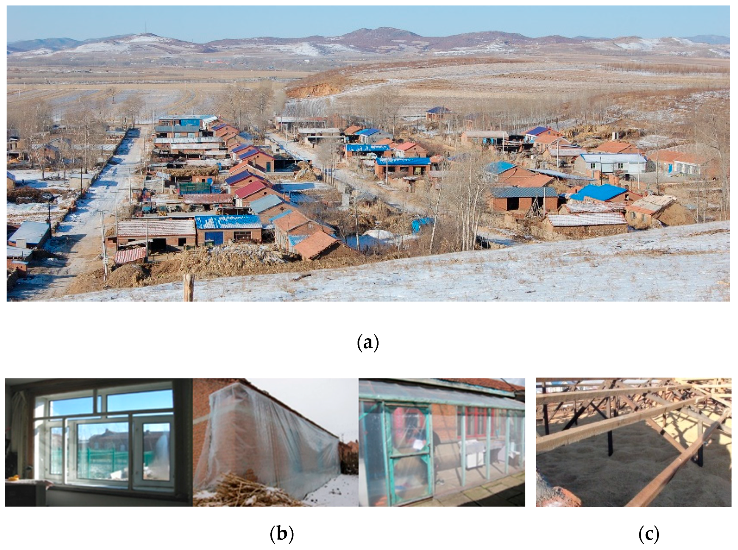
Figure 3.
Kang heating system with fire wall.

Figure 4.
Tested house and arrangement of monitoring points: (a) appearance; (b) monitoring point arrangement; (c) living room; (d) heating equipment; (e) condensation; (f) heat transfer coefficient test.
Figure 4.
Tested house and arrangement of monitoring points: (a) appearance; (b) monitoring point arrangement; (c) living room; (d) heating equipment; (e) condensation; (f) heat transfer coefficient test.
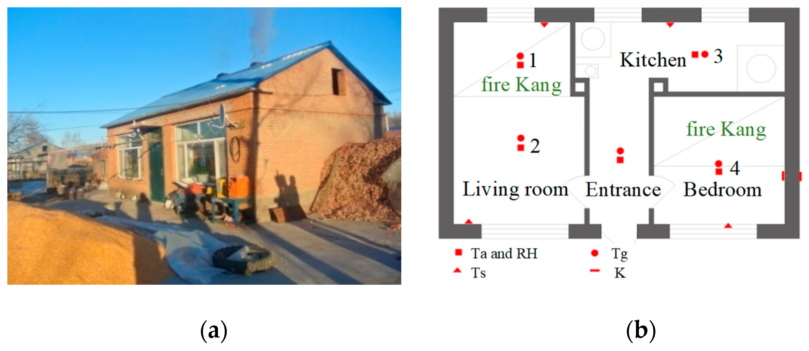
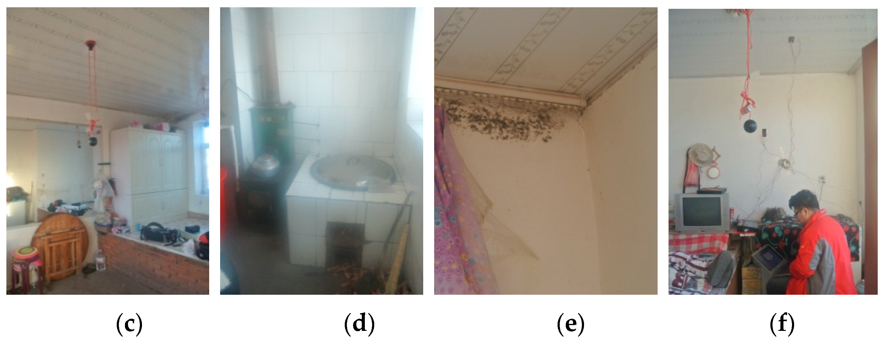
Figure 5.
Point distribution of the orthogonal experiments.
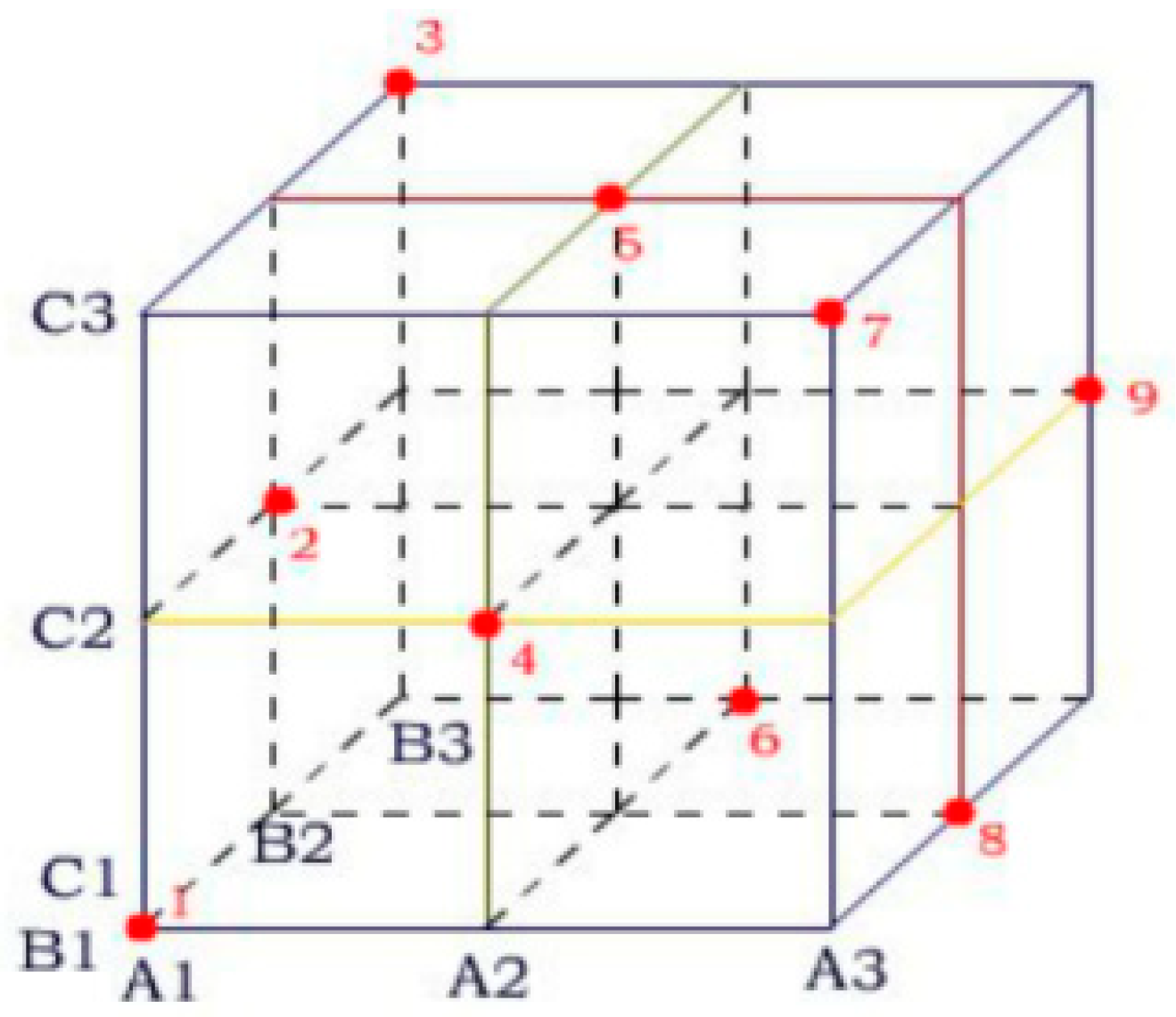
Figure 6.
Indoor and outdoor (a) temperature and (b) relative humidity.

Figure 7.
Comparison of surface temperature and indoor temperature.

Figure 8.
Infrared thermal imaging of the corner of the building envelope.

Figure 9.
Differences between indoor air and globe temperatures.
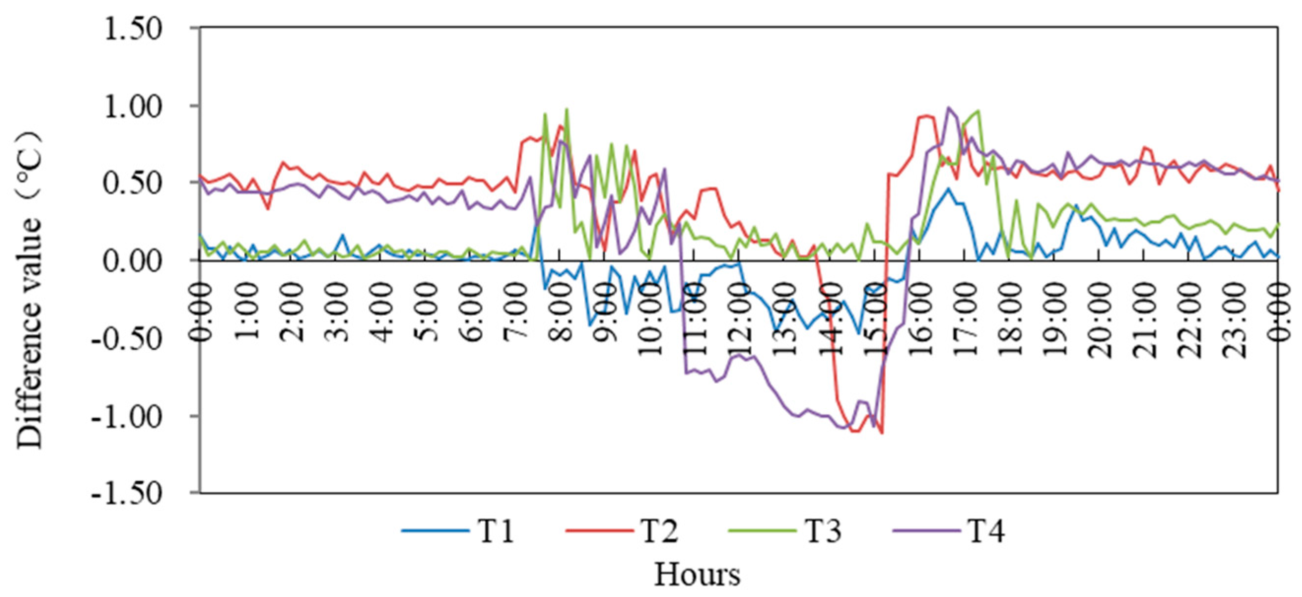
Figure 10.
Distribution of clothing thermal resistance.
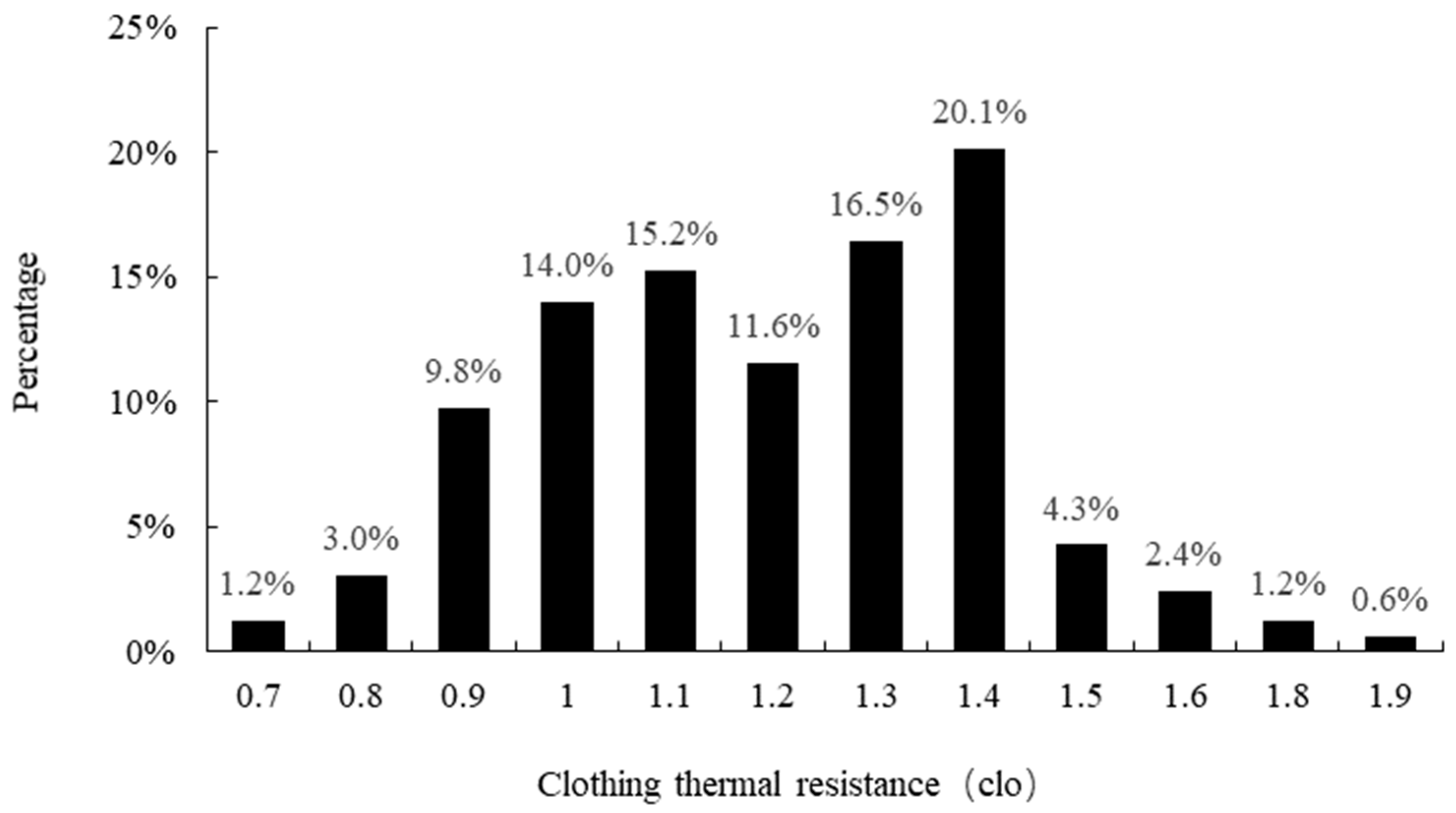
Figure 11.
Distribution of air temperature.

Figure 12.
Distribution of mean radiant temperature.
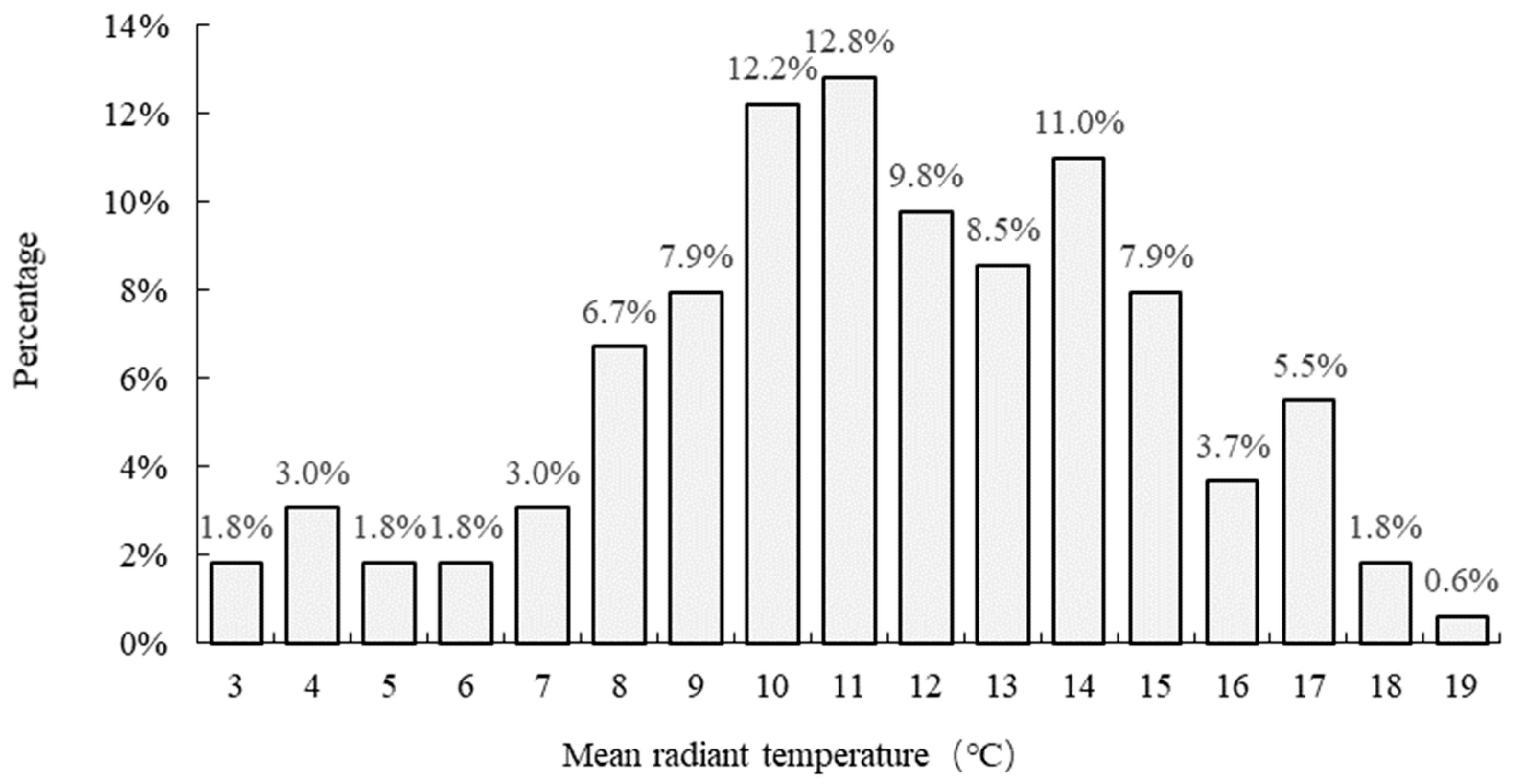
Figure 13.
Distribution of the thermal sensation vote and its relation between mean thermal acceptability.
Figure 13.
Distribution of the thermal sensation vote and its relation between mean thermal acceptability.

Figure 14.
Distribution of thermal acceptability.
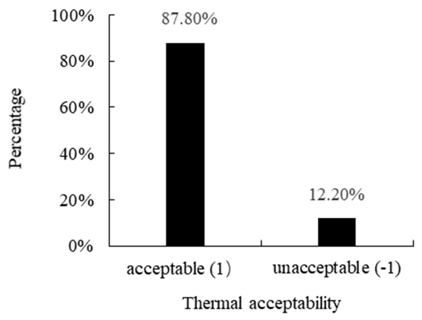
Figure 15.
Distribution of thermal preference.
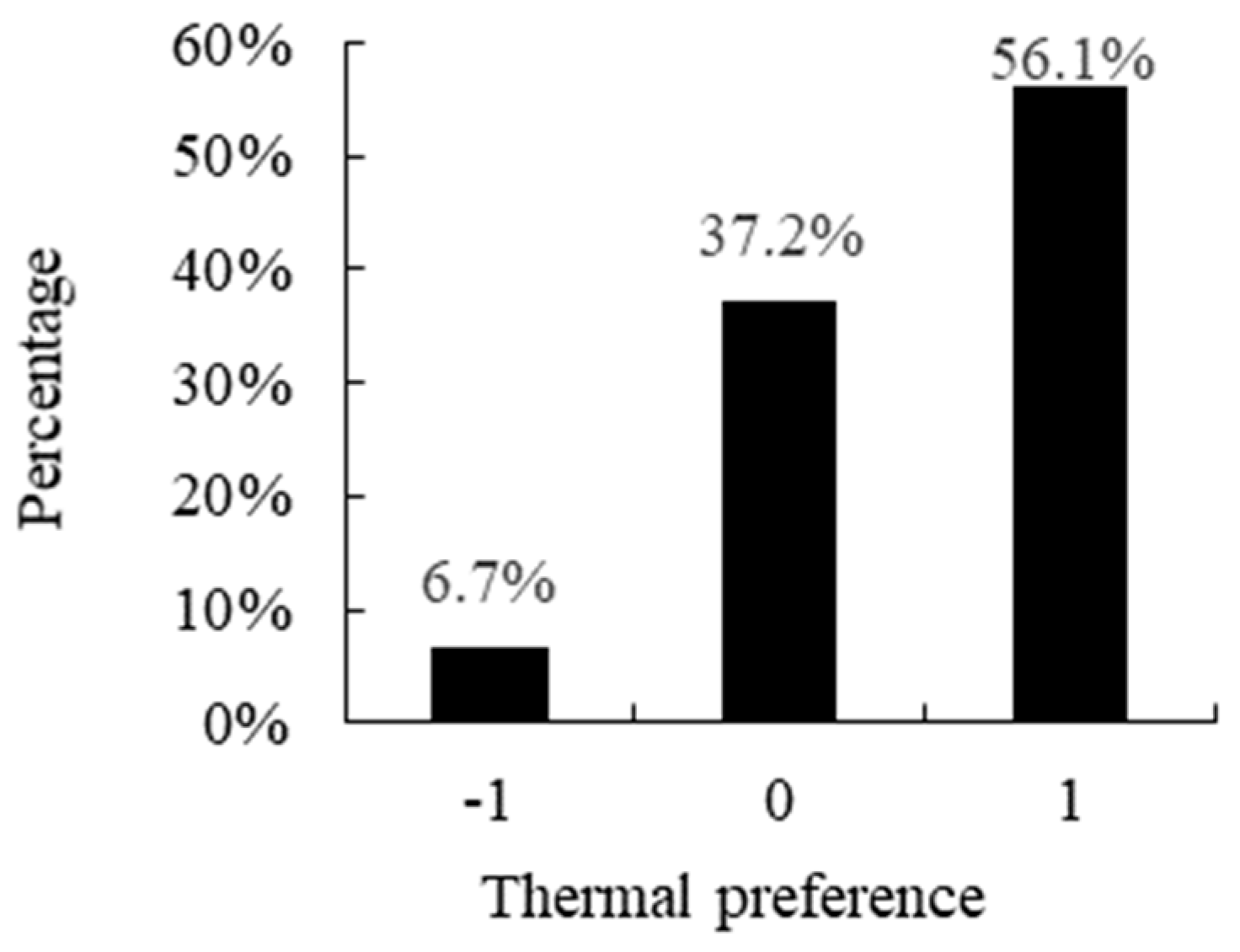
Figure 16.
Relationship between thermal sensation vote (TSV) and thermal preference.
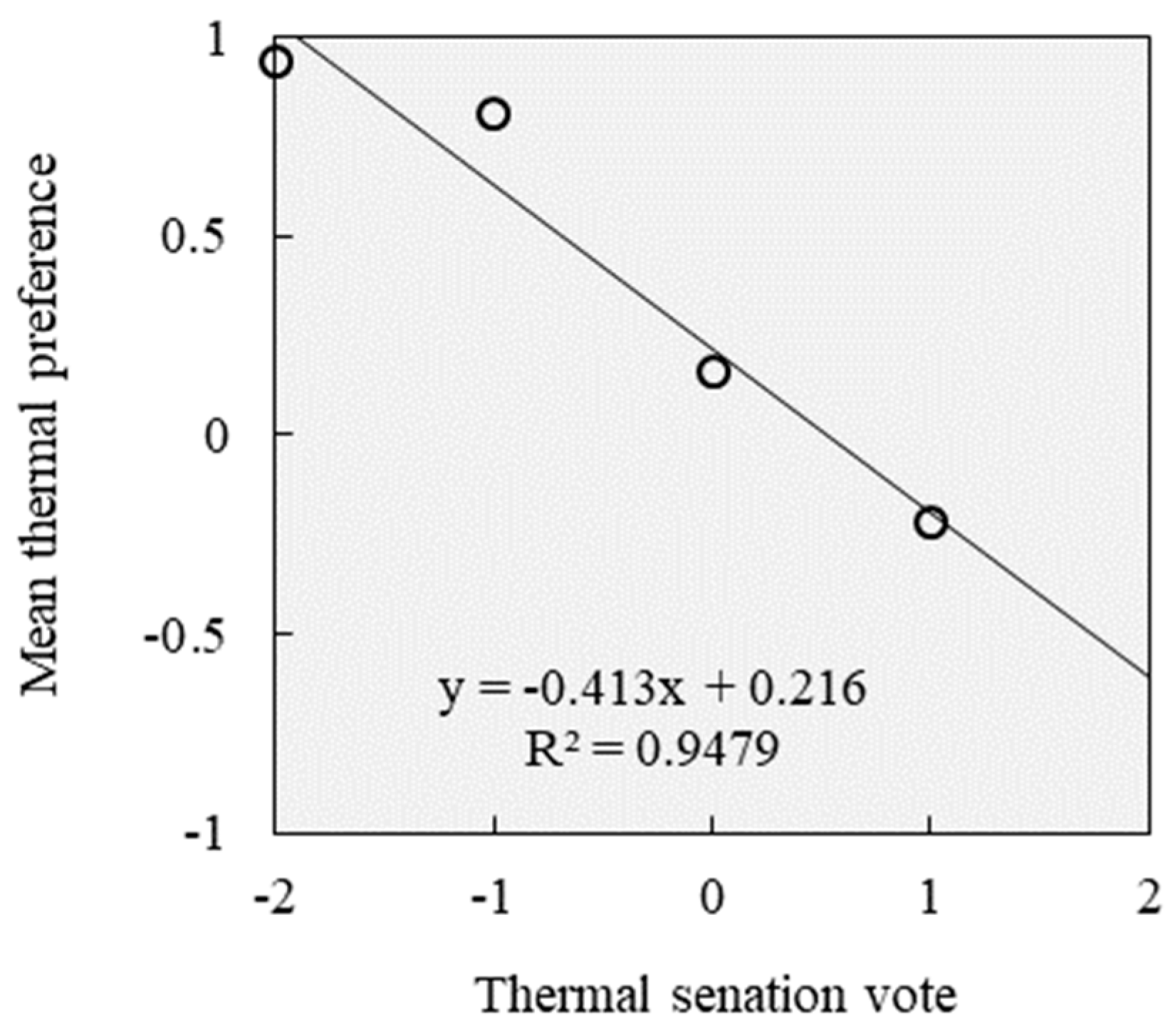
Figure 17.
Relationship between mean thermal sensation (MTS) and operative temperatures.

Figure 18.
Relationship between building orientation and heating energy consumption and solar radiation heating.
Figure 18.
Relationship between building orientation and heating energy consumption and solar radiation heating.
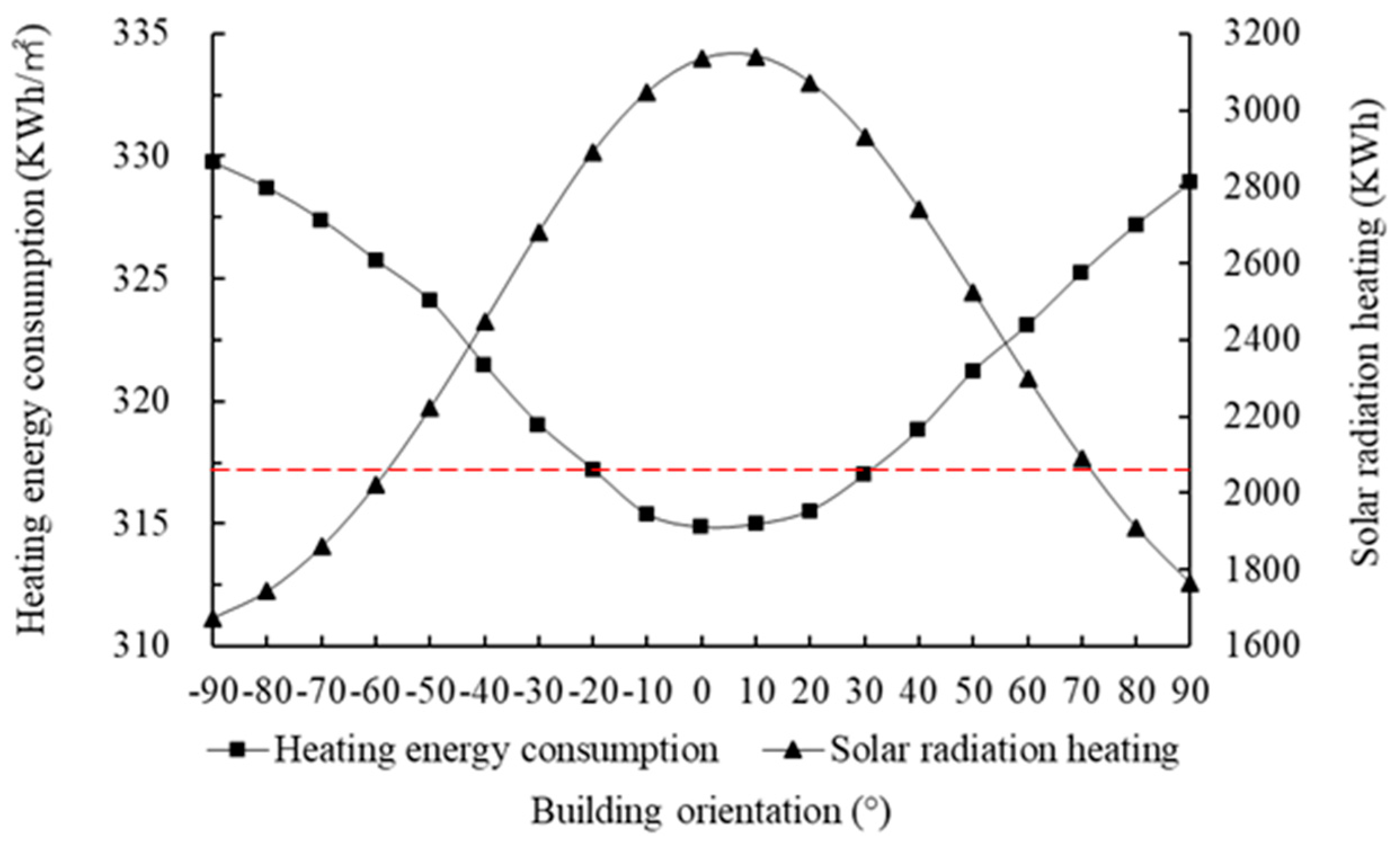
Figure 19.
Relationship between the length–width ratio and energy consumption.
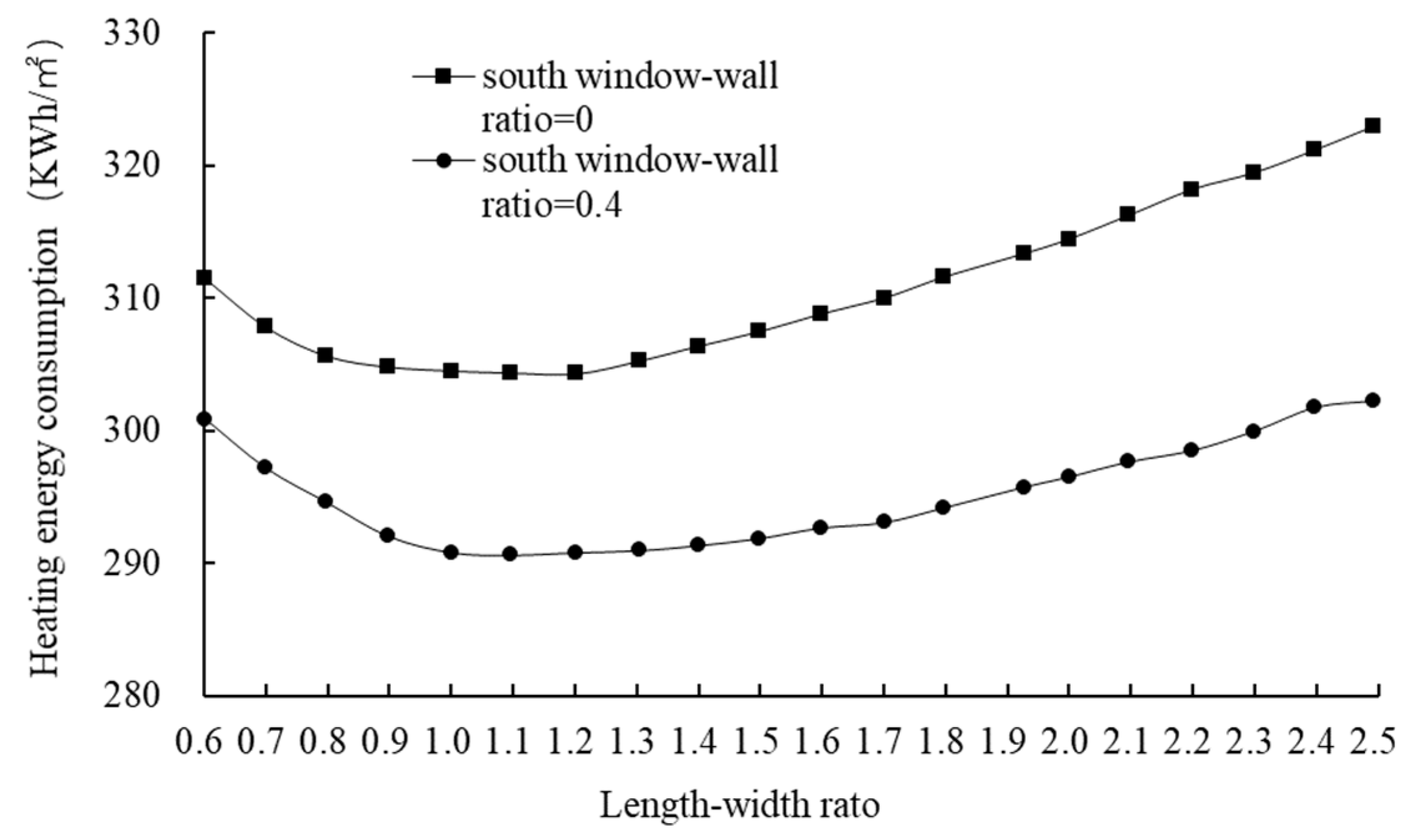
Figure 20.
Relationship between indoor height and energy consumption.

Figure 21.
Relationship between insulation layer thickness and heating energy consumption.
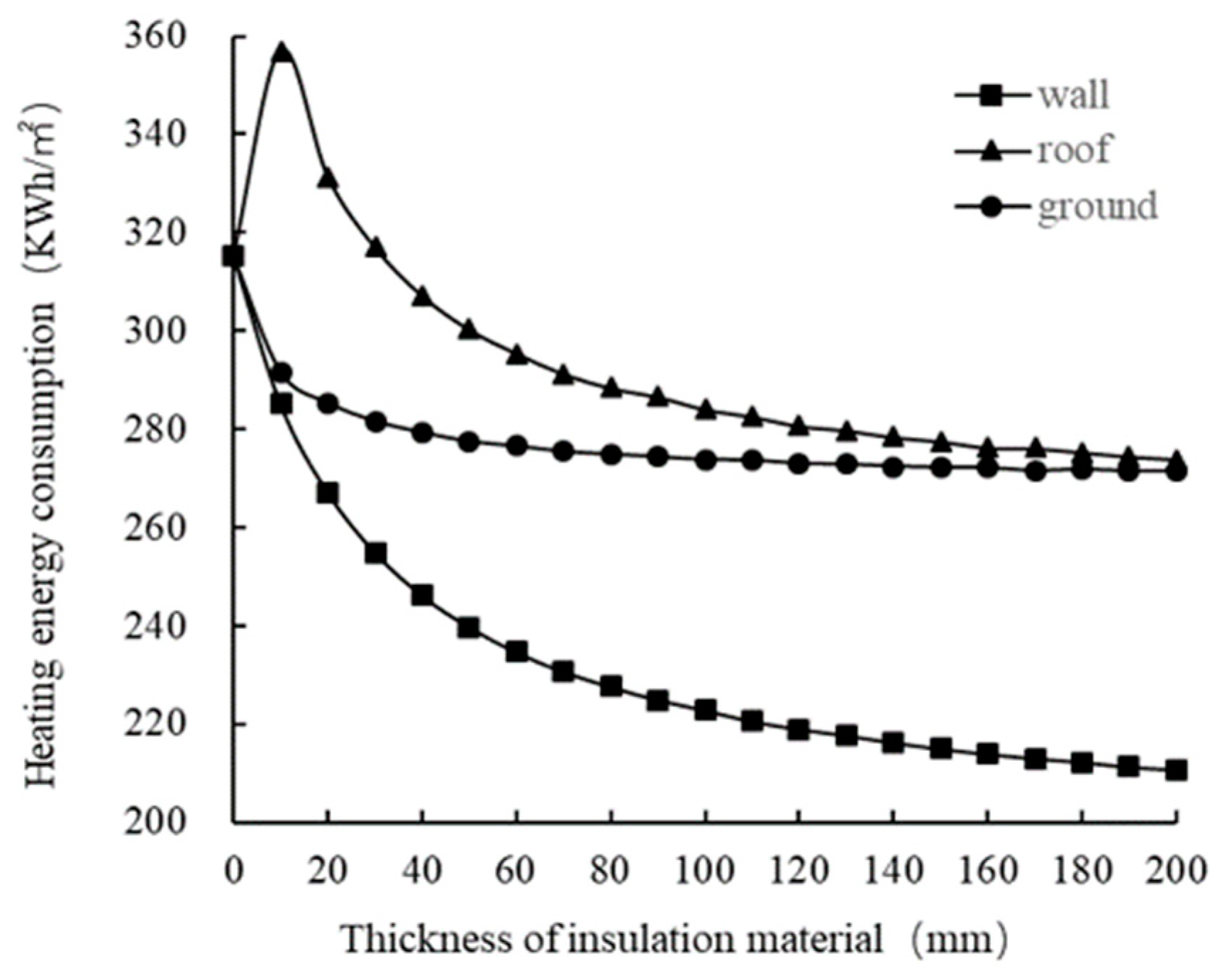
Figure 22.
Relationship between insulation layer thickness and energy-saving rate.
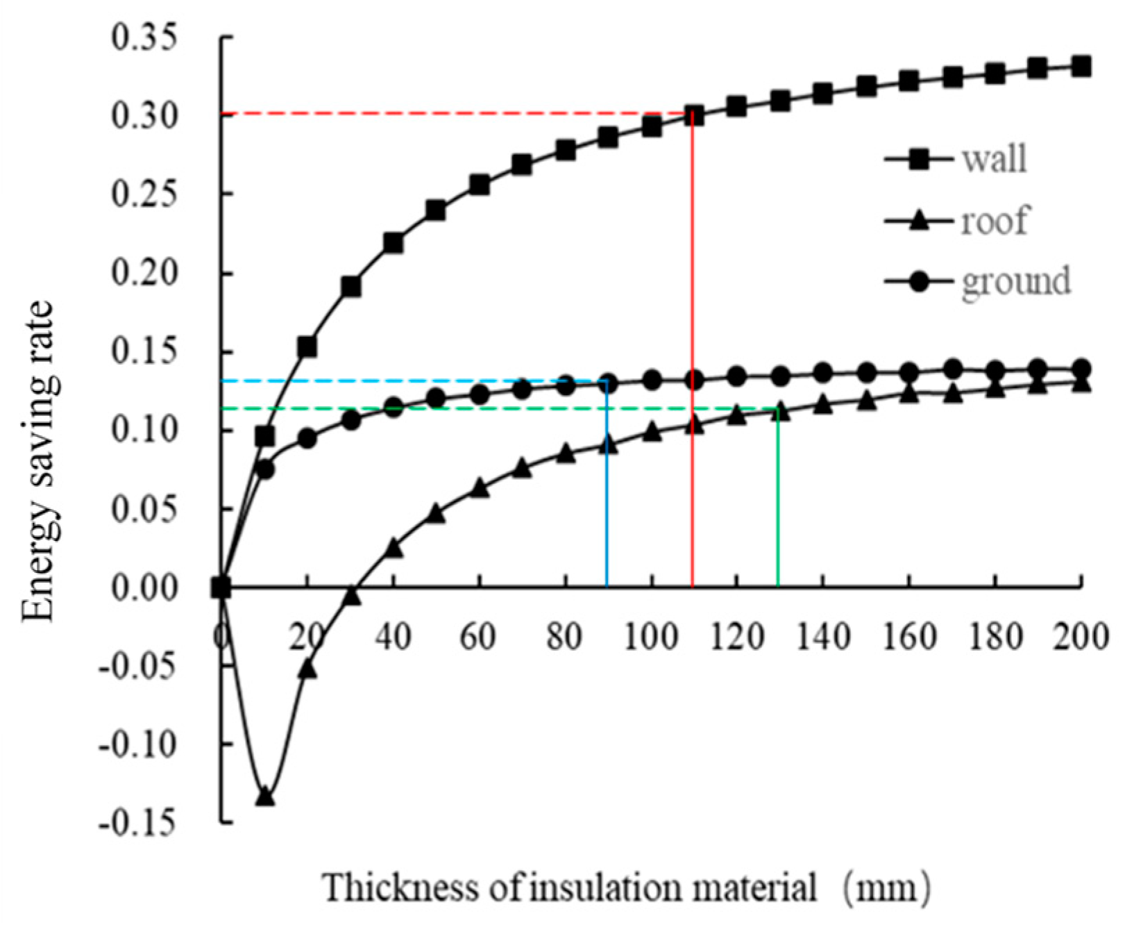
Figure 23.
Relationship between window thermal performance and energy consumption and solar radiation.
Figure 23.
Relationship between window thermal performance and energy consumption and solar radiation.

Figure 24.
Relationship between the south window–wall ratio and energy consumption and solar radiation.
Figure 24.
Relationship between the south window–wall ratio and energy consumption and solar radiation.

Figure 25.
Relationship between the north window–wall ratio and energy consumption and solar radiation.
Figure 25.
Relationship between the north window–wall ratio and energy consumption and solar radiation.
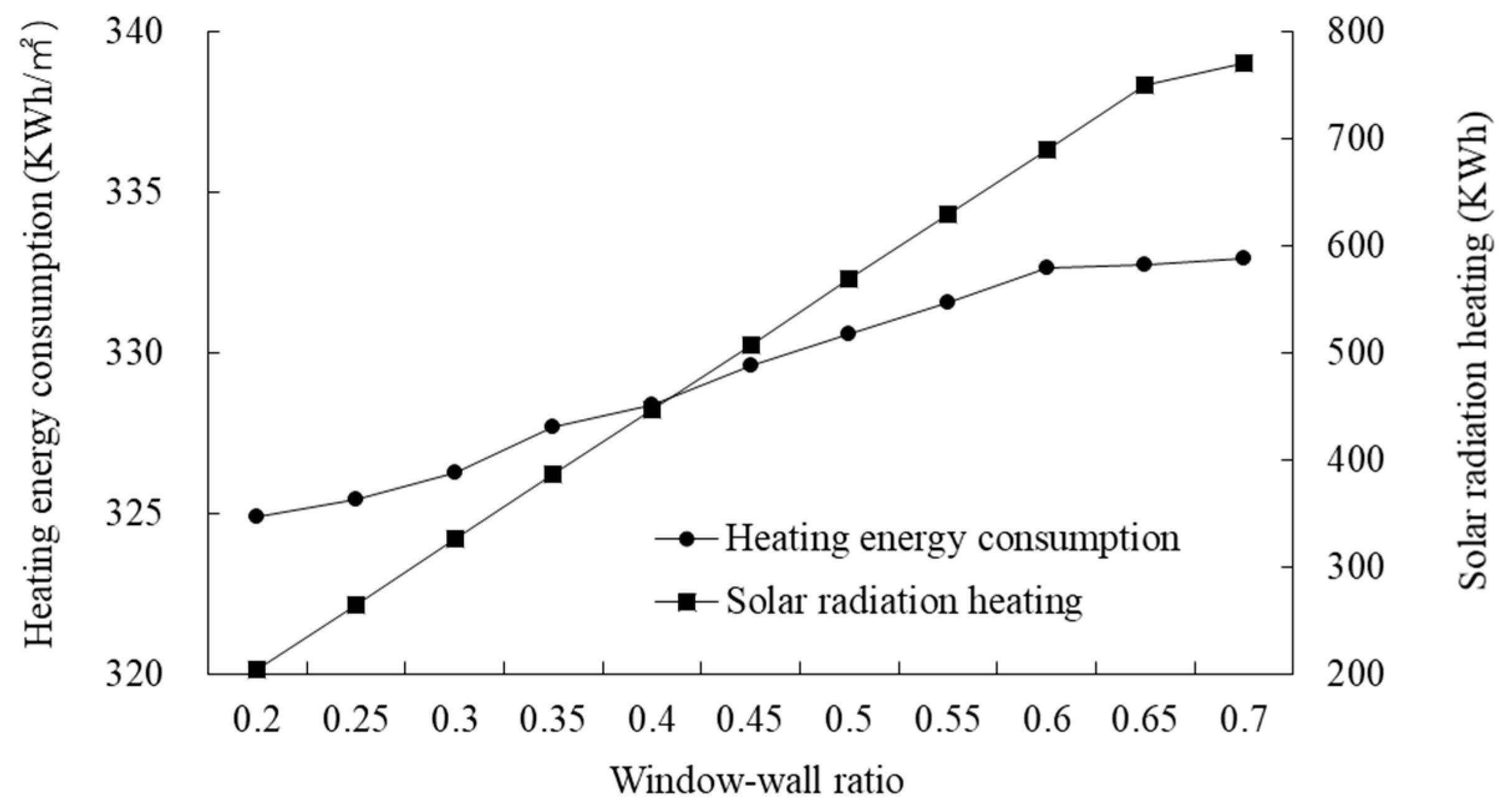
Figure 26.
Building model with a sunspace.
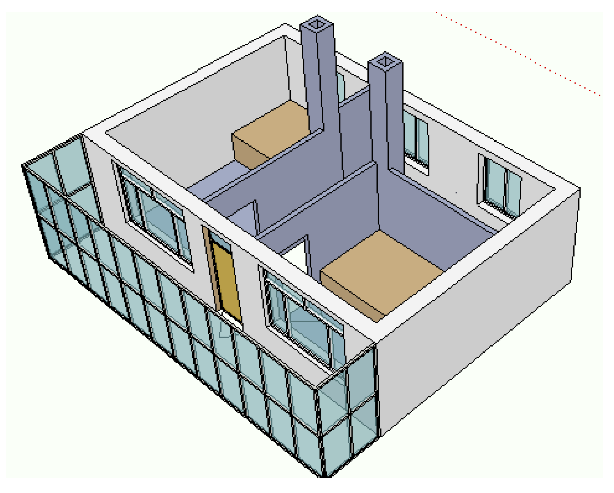
Figure 27.
The attached sunspace of a rural house.
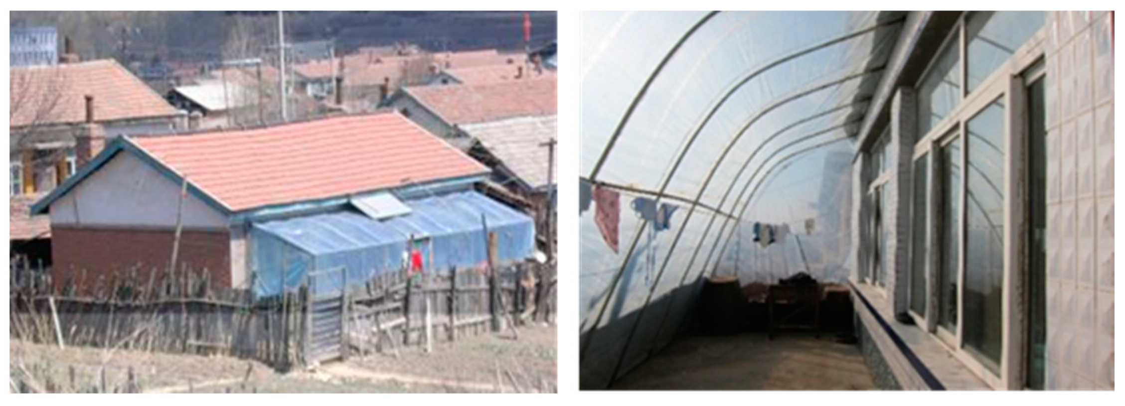
Figure 28.
Relationship between sunspace depth and heating energy consumption.
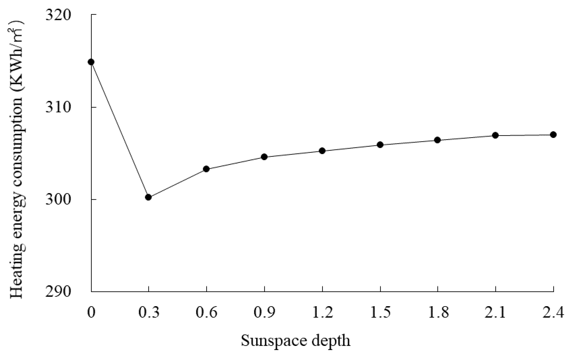
Figure 29.
Reduction of solar radiation and heat loss of the envelope.

Figure 30.
Indoor, sunspace, and outdoor mean air temperature in winter.
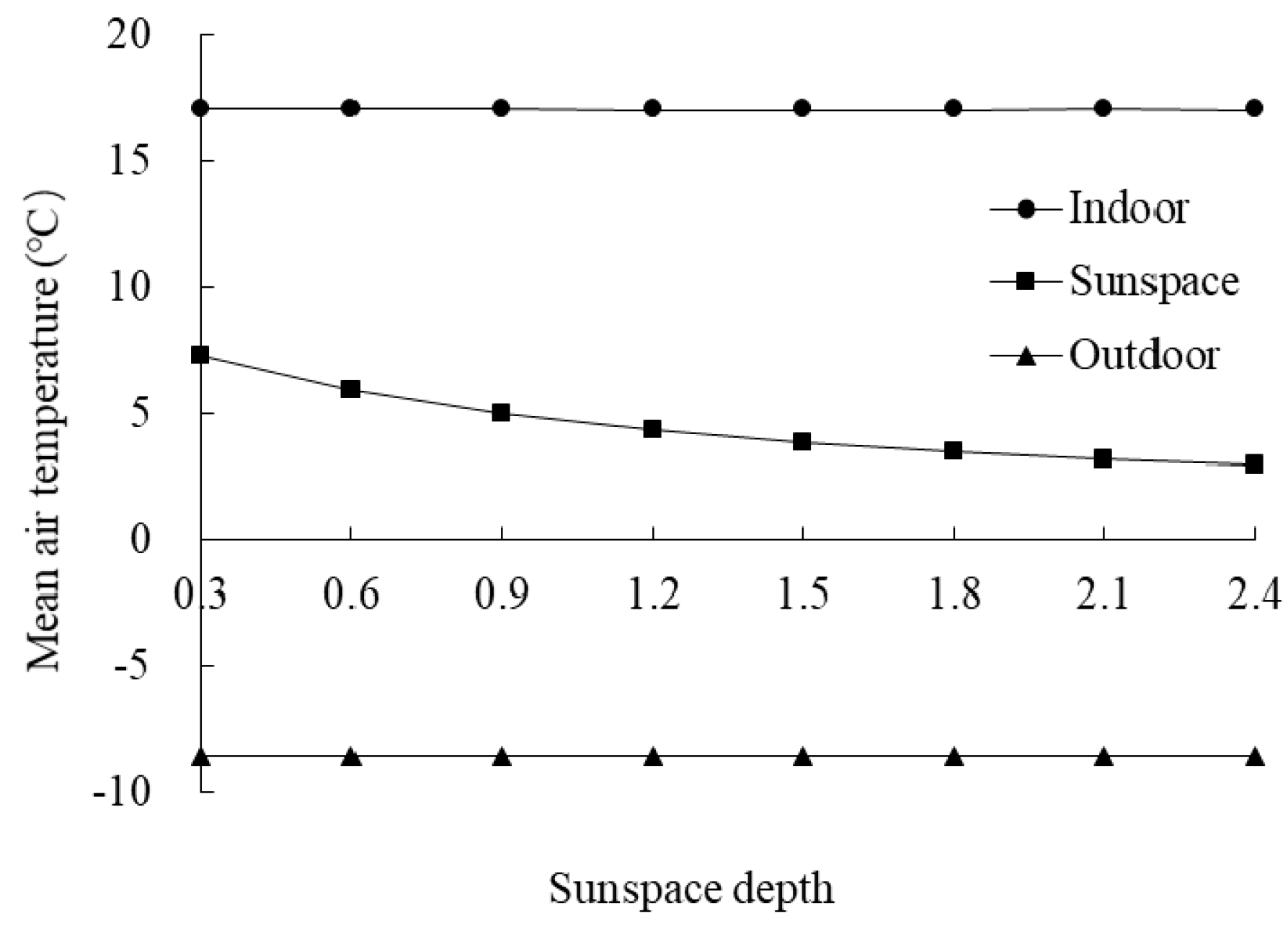
Figure 31.
Distribution of investment cost for energy-saving design or reconstruction.

Table 1.
Instruments used for measurement of the thermal environment.
| Parameter | Model | Range | Accuracy |
|---|---|---|---|
| Air temperature (Ta) and relative humidity (RH) | BES-02 | −30 to 50 °C, 0–99% | ±0.5 °C, ±3% |
| Surface temperature (Ts) | BES-01 (external sensor) | −30 to 50 °C | ±0.5 °C |
| Globe temperature (Tg) | BES-01 (external black globe, diameter 0.15 m) | −30 to 50 °C | ±0.5°C |
| Wind speed (V) | KANOMAX | 0.01–20 m/s | ±0.01 m/s |
| Heat transfer coefficient (K) | BES-Aa | −40 to 100 °C, 0–±20 mV | ±0.2 °C, ±0.01 mV |
| Infrared thermal imaging | Fluke | −20 to 550 °C | ±2°C |
Table 2.
Distribution characteristics of the indoor thermal environment parameters.
| Parameter | Mean Value | Standard Deviation | Max Value | Min Value |
|---|---|---|---|---|
| Air temperature (°C) | 15.0 | 3.39 | 22.0 | 7.0 |
| Mean radiant temperature (°C) | 11.0 | 3.47 | 19.0 | 3.0 |
| Relative humidity (%) | 51.0 | 11.04 | 75.0 | 22.0 |
| Air velocity (m/s) | 0.02 | 0.01 | 0.06 | 0.01 |
Table 3.
Operative temperature range and mean thermal sensation vote.
| Operating Temperature | MTS | Operating Temperature | MTS | Operating Temperature | MTS | Operating Temperature | MTS |
|---|---|---|---|---|---|---|---|
| 4.75 | −2 | 8.75 | −1 | 12.75 | −0.45 | 16.75 | 0 |
| 5.25 | −2 | 9.25 | −1.25 | 13.25 | −0.44 | 17.25 | 0 |
| 5.75 | −2 | 9.75 | −1.25 | 13.75 | −0.63 | 17.75 | 0 |
| 6.25 | −2 | 10.25 | −1 | 14.25 | −0.44 | 18.25 | 0 |
| 6.75 | −2 | 10.75 | −1 | 14.75 | −0.33 | 18.75 | 0.4 |
| 7.25 | −2 | 11.25 | −0.9 | 15.25 | −0.38 | 19.25 | 1 |
| 7.75 | −2 | 11.75 | −1.2 | 15.75 | −0.1 | 19.75 | 1 |
| 8.25 | −2 | 12.25 | −0.7 | 16.25 | 0 | 20.25 | 1 |
Table 4.
Typical structure of the building envelope [60].
Table 4.
Typical structure of the building envelope [60].
| Name | Diagram | Structures |
|---|---|---|
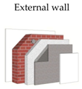 | 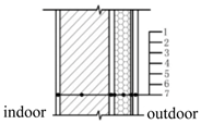 | 1. Interior surface 2. 370 mm solid brick 3. Cement mortar 4. Cementing compound 5. EPS board 6. Alkali resistant glass fiber mesh cloth (8 mm, double layer) 7. Exterior surface |
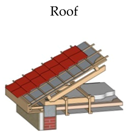 | 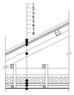 | 1. Tile 2 Waterproof layer 3. Plank 4. Wood (or steel) roof truss 5. EPS board 6. Vapor barrier (plastic film) 7. Wood joist 8. Suspended ceiling |
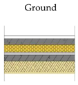 |  | 1. Surface course 2. Protective layer 3. EPS board 4. Damp roof course 5. 20 mm cement mortar 6. 100 mm concrete cushion 7. Rammed earth |
Table 5.
External window types and parameters. K, heat transfer coefficient; SHGC, solar heat gain coefficient; low-e, low emissivity; A, air.
Table 5.
External window types and parameters. K, heat transfer coefficient; SHGC, solar heat gain coefficient; low-e, low emissivity; A, air.
| Number | Window Type | K | SHGC |
|---|---|---|---|
| 1 | 6 mm clear + 6A + 6 mm clear | 3.1 | 0.700 |
| 2 | 6 mm clear + 6A + 6 mm bronze | 3.1 | 0.504 |
| 3 | 6 mm clear + 6A + 6 mm gray | 3.1 | 0.485 |
| 4 | 6 mm clear + 12A + 6 mm clear | 2.7 | 0.715 |
| 5 | 6 mm clear + 6A + 6 mm low-e | 2.4 | 0.569 |
| 6 | 6 mm clear + 6A + 6 mm clear + 6A + 6 mm clear | 2.1 | 0.624 |
| 7 | 6 mm g clear + 6A + 6 mm clear + 100A + 6 mm clear + 6A + 6 mm clear | 1.5 | 0.554 |
Table 6.
Correlation between window thermal performance and energy consumption.
| K (W/m2·K) | SHGC | |
|---|---|---|
| Pearson correlation | 0.949 ** | −0.296 |
| Significance (bilateral) | 0.001 | 0.520 |
** Significant correlation at the 0.01 level (bilateral).
Table 7.
Fitting relationship between the window–wall ratio and energy consumption.
| Regression Equation | Regression Coefficient (R2) | Significance Test (Sig.) | |
|---|---|---|---|
| South window–wall ratio | Y = −35.164X + 321.594 | 0.998 | 0.000 |
| North window–wall ratio | Y = 17.876X + 321.286 | 0.980 | 0.000 |
Table 8.
Factors and levels of the orthogonal experiments.
| Level | Factor | |||||||||
|---|---|---|---|---|---|---|---|---|---|---|
| A | B | C | D | E | F | G | H | I | J | |
| 1 | South by west 20° | 1.0 | 2.6 | 50 | 70 | 30 | 1.5 | 0.3 | 0.1 | 0.9 |
| 2 | South by west 10° | 1.1 | 2.7 | 70 | 90 | 50 | 2.1 | 0.4 | 0.2 | 1.2 |
| 3 | South (0°) | 1.2 | 2.8 | 90 | 110 | 70 | 2.4 | 0.5 | 0.3 | 1.5 |
| 4 | South by east 10° | 1.3 | 2.9 | 110 | 130 | 90 | 2.7 | 0.6 | 0.4 | 1.8 |
Note: A: building orientation (°); B: length–width ratio; C: indoor height (m); D: external wall insulation thickness (mm); E: roof insulation thickness (mm); F: ground insulation thickness (mm); G: window heat transfer coefficient of (W/m2·K); H: south window–wall ratio; I: north window–wall ratio; J: sunspace depth (m).
Table 9.
Range calculation results of the orthogonal experiments.
| Mean Value (KWh/m²) | Factors | ||||||||||
|---|---|---|---|---|---|---|---|---|---|---|---|
| A | B | C | D | E | F | G | H | I | J | Blank Column | |
| 143.55 | 142.79 | 137.61 | 154.93 | 152.81 | 148.84 | 137.47 | 142.50 | 137.46 | 141.86 | 142.94 | |
| 142.83 | 142.75 | 140.81 | 144.85 | 143.90 | 143.59 | 142.75 | 142.90 | 141.52 | 142.97 | 143.28 | |
| 143.28 | 143.29 | 144.62 | 138.42 | 139.46 | 140.89 | 146.21 | 143.44 | 144.84 | 143.57 | 143.10 | |
| 143.21 | 144.04 | 149.83 | 134.66 | 136.71 | 139.55 | 146.44 | 144.03 | 149.04 | 144.47 | 143.55 | |
| Ri | 0.72 | 1.29 | 12.22 | 20.27 | 16.10 | 9.29 | 8.97 | 1.53 | 11.58 | 2.61 | 0.61 |
Note: A: building orientation (°); B: length–width ratio; C: indoor height (m); D: external wall insulation thickness (mm); E: roof insulation thickness (mm); F: ground insulation thickness (mm); G: window heat transfer coefficient (W/m2·K); H: south window–wall ratio; I: north window–wall ratio; J: sunspace depth (m).
Table 10.
Temperature distribution over one year, 8760 h.
| ≤17 °C | 17–21 °C | 21–26 °C | <26 °C | |
|---|---|---|---|---|
| Ambient temperature (h) | 6295 | 974 | 1059 | 432 |
| Indoor temperature (h) | 6198 | 2106 | 456 | 0 |
| After energy-saving design (h) | 5125 | 1152 | 2121 | 362 |
Table 11.
ANOVA of the building energy-consumption data.
| III Type Quadratic Sum | df | MS | F | Sig. | |
|---|---|---|---|---|---|
| A: Building orientation | 4.233 | 3 | 1.411 | 0.246 | 0.864 |
| B: Length–width ratio | 17.113 | 3 | 5.704 | 0.993 | 0.409 |
| C: Indoor height | 1326.900 | 3 | 442.300 | 76.995 | 0.000 |
| D: External wall insulation thickness | 3779.036 | 3 | 1259.679 | 219.282 | 0.000 |
| E: Roof insulation thickness | 2383.959 | 3 | 794.653 | 138.331 | 0.000 |
| F: Ground insulation thickness | 810.240 | 3 | 270.080 | 47.015 | 0.000 |
| G: Window heat transfer coefficient | 840.762 | 3 | 280.254 | 48.786 | 0.000 |
| H: South window–wall ratio | 21.333 | 3 | 7.111 | 1.238 | 0.313 |
| I: North window–wall ratio | 1161.877 | 3 | 387.292 | 67.419 | 0.000 |
| J: Sunspace depth | 57.550 | 3 | 19.183 | 3.339 | 0.032 |
| K: Blank column | 3.278 | 3 | 1.093 | 0.190 | 0.902 |
| Deviation | 172.337 | 30 | 5.745 |
Table 12.
The increased investment cost of an energy-saving house.
| Parts | Additional or Replacement Material | Price | Area (m2) | Difference in Investment Cost (CNY) | ||
|---|---|---|---|---|---|---|
| Wall | EPS | 360 CNY/m3 | 67.20 | 2661.1 | ||
| Roof | EPS | 360 CNY/m3 | 54.12 | 2532.8 | ||
| Ground | EPS | 360 CNY/m3 | 54.12 | 1753.5 | ||
| Sunspace | Single-glass with aluminum alloy frame | 120 CNY/m2 | 31.63 | 3795.6 | ||
| Window replacement | Reference building | Single-frame double-glass window | 270 CNY/m2 | 14.04 | 3790.8 | 118.8 |
| Energy-saving house | Two single-frame double-glass window | 540 CNY/m2 | 7.24 | 3909.6 | ||
| Total | 10,861.8 | |||||
Note: Additional materials are for external walls, roof, ground, and sunspace. Replacement materials are for external windows and the area changed. Labor cost is included in the price of the materials.
© 2020 by the authors. Licensee MDPI, Basel, Switzerland. This article is an open access article distributed under the terms and conditions of the Creative Commons Attribution (CC BY) license (http://creativecommons.org/licenses/by/4.0/).
Share and Cite
MDPI and ACS Style
Shao, T.; Zheng, W.; Jin, H. Analysis of the Indoor Thermal Environment and Passive Energy-Saving Optimization Design of Rural Dwellings in Zhalantun, Inner Mongolia, China. Sustainability 2020, 12, 1103. https://doi.org/10.3390/su12031103
AMA Style
Shao T, Zheng W, Jin H. Analysis of the Indoor Thermal Environment and Passive Energy-Saving Optimization Design of Rural Dwellings in Zhalantun, Inner Mongolia, China. Sustainability. 2020; 12(3):1103. https://doi.org/10.3390/su12031103
Chicago/Turabian StyleShao, Teng, Wuxing Zheng, and Hong Jin. 2020. "Analysis of the Indoor Thermal Environment and Passive Energy-Saving Optimization Design of Rural Dwellings in Zhalantun, Inner Mongolia, China" Sustainability 12, no. 3: 1103. https://doi.org/10.3390/su12031103
Note that from the first issue of 2016, this journal uses article numbers instead of page numbers. See further details here.