Article

Evaluation Indexes and Correlation Analysis of Origination–Destination Travel Time of Nanjing Metro Based on Complex Network Method

1
College of Automobile and Traffic Engineering, Nanjing Forestry University, Longpan Road 159#, Nanjing 210037, China
2
School of Maritime and Transportation, Ningbo University, Fenghua Road 818#, Ningbo 315211, China
3
School of Transportation, Southeast University, Southeast University Road 2#, Nanjing 210096, China
4
School of Architecture and Transportation, Guilin University of Electronic Technology, Jinji Road 1#, Guilin 541004, China
*
Author to whom correspondence should be addressed.
Sustainability 2020, 12(3), 1113; https://doi.org/10.3390/su12031113
Submission received: 19 January 2020 / Revised: 30 January 2020 / Accepted: 3 February 2020 / Published: 4 February 2020

Abstract

:
The information level of the urban public transport system is constantly improving, which promotes the use of smart cards by passengers. The OD (origination–destination) travel time of passengers reflects the temporal and spatial distribution of passenger flow. It is helpful to improve the flow efficiency of passengers and the sustainable development of the city. It is an urgent problem to select appropriate indexes to evaluate OD travel time and analyze the correlation of these indexes. More than one million OD records are generated by the AFC (Auto Fare Collection) system of Nanjing metro every day. A complex network method is proposed to evaluate and analyze OD travel time. Five working days swiping data of Nanjing metro are selected. Firstly, inappropriate data are filtered through data preprocessing. Then, the OD travel time indexes can be divided into three categories: time index, complex network index, and composite index. Time index includes use time probability, passenger flow between stations, average time between stations, and time variance between stations. The complex network index is based on two models: Space P and ride time, including the minimum number of rides, and the shortest ride time. Composite indicators include inter site flow efficiency and network flow efficiency. Based on the complex network model, this research quantitatively analyzes the Pearson correlation of the indexes of OD travel time. This research can be applied to other public transport modes in combination with big data of public smart cards. This will improve the flow efficiency of passengers and optimize the layout of the subway network and urban space.

1. Introduction

As the city scale expands, the integrated transportation system will become more and more complex to meet the travel needs of different residents. With the development of the economy and the expansion of the population, the subway has been opened in many cities in China to relieve the increasing traffic pressure. Smart cards have been widely used in the integrated transportation system, recording the electronic information of passengers’ travel. Smart card data records the station and time when passengers enter and leave the station, which is called the OD (origination–destination) record. The smart card big data accumulated by the AFC (Automatic Fare Collection) system provides the basis for the analysis of urban residents’ travel behavior.
OD records reflect the destination needs of residents. Kim H proposed an OD estimation model based on multi-source data, which can identify the travel demand of the destination [1]. Kim K established a spatiotemporal autoregressive model of air passenger flow from the origin to the destination in order to better plan and dispatch the operation, and has verified the effectiveness of the model in predicting air passenger flow [2]. Zhang C used the track data to track the OD mode of vehicle movement, and proposed a measurement method based on the on ramp flow. Compared with the traditional method of fixed sensors, it improves the measurement accuracy [3].
Liu L proposed a new spatiotemporal network model to analyze the evolution of taxi demand. The results show that this method can predict the demand of the taxi destination better [4]. Bachir D used mobile network data, combined with transportation network geospatial data, tourism survey, census and tourism card data, to infer the user’s dynamic departure destination [5]. Mungthanya W proposed a new method to construct a dynamic OD matrix of taxi in space and time by using taxi trajectory data, and analyzed the demand mode of taxi travel [6].
The OD data of passengers is extracted and distributed to the traffic line, which can analyze the passenger flow pressure on the traffic line. Javani B proposed an OD based on the algorithm for static traffic assignment with fixed OD demand, which is tested in Chicago and Philadelphia [7]. Mehrabipour M proposed a multi OD algorithm based on the cell transmission model, which can optimize the dynamic traffic assignment of the system [8]. Hoang N H proposed a new linear programming framework, which uses the relationship between UE (user equilibrium) and the system optimal solution to solve the dynamic traffic assignment problem [9].
OD records can be combined with the passenger’s travel preferences to determine the passenger’s travel path choice. Wang Y proposed a two-stage algorithm, which uses the traffic flow data of link level to accurately estimate the OD matrix and improves the traveler’s path selection behavior model [10]. Based on long-term GPS (global positioning system) data, Li D introduced OD attribute and used utility function to explore the influence of destination attribute on path selection [11]. Ou J proposed a new framework for estimating dynamic OD flow using machine learning algorithm, and carried out an evaluation experiment on the real network of Kunshan City [12]. Duan Z proposed a hybrid neural network prediction model, which can effectively predict the OD traffic of the urban taxi [13].
In order to evaluate OD, it is necessary to set various indexes to evaluate passengers’ behaviors quantitatively. Yang S used taxi GPS data to estimate OD travel time, which helps to analyze the route preference of passengers [14]. Margaretic P applied the spatial economic flow model and characteristic function spatial filtering method to air transportation, and discussed the impact of departure destination on air passenger flow [15]. Hanseler F S proposed a framework for estimating pedestrian demand in railway stations, which considers passenger data and various direct and indirect demand indicators [16].
Nigro M collected all the monitoring travel data of specific areas in Rome of Italy, and analyzed the travel time and route selection probability of the passenger’s OD, which can improve the temporal and spatial reliability of the demand matrix [17]. Ma W used the daily traffic data collected over the years to propose a new theoretical framework, which is used to consider the daily changes caused by travelers’ independent choice of routes and estimate OD demand, path selection probability, and travel cost [18]. Dai X proposed a data-driven short-term subway passenger flow prediction framework, which can be successfully used to describe different subway travel modes [19].
Sensor technology can also be used to locate vehicles and predict traffic flow. Wang J proposed a Bayesian combination method to predict traffic flow [20]. Zhu S proposed a sensor location model to determine the optimal deployment strategy for dynamic origination–destination demand estimation [21]. Zhu N proposed a two-stage stochastic model to estimate the travel time of the highway corridor [22]. Hobson B W used sensors to estimate occupancy of commercial and institutional buildings [23].
Passenger’s identity, policy, environment, and other factors will affect passenger’s travel choice. Moslem S proposed a decision support program that can analyze and build consensus among different stakeholders in traffic development issues [24]. Ghorbanzadeh O used an interval level method to analyze the inconsistency and uncertainty of the public transport user’ response [25]. Duleba S used the analytic hierarchy method to analyze the significance of stakeholders in Mersin, Turkey [26]. Duleba S used the analytic hierarchy method combined with real data to test the optimal public transport service [27]. Moslems used the fuzzy analytic hierarchy method to analyze the sustainable development of urban traffic in Mersin, Turkey [28]. Jiang X used the improved fuzzy analytic hierarchy process to analyze the most basic factors affecting the last kilometer distribution [29].
Guo Y used the collected data of residents’ travel preferences to study the impact of domestic mobility, the household registration system, and family planning policy on passengers’ travel patterns [30]. Ruan Y analyzed the differences between daily life and pre migration, the difficulties encountered after migration and the social adaptation pressure of the floating elderly [31]. Guo Y analyzed the impact of the information provided to potential relocaters on their decision-making process and travel behavior after relocation [32]. Li Y studied the effects of congestion pricing and incentive strategies on early travel mode choice of car travelers in Beijing [33].
Based on the moving data of Beijing’s families, Wang D linked the residential building environment with travel behavior, and considered travel attitude before and after the housing change [34]. Cheng G investigated the tourism preferences of residents in two underdeveloped small cities, analyzed the tourism data of different regions, and discussed their commonness [35]. Using the data of passengers’ travel behavior, Guo Y explored the personal and social impact of the ban on motorcycles on the morning commuting of motorcyclists’ families [36].
The establishment of the complex network model of the subway is an effective way to analyze the performance of the urban subway network. Feng J proposed a weighted complex network model based on travel data and the operation schedule of the Beijing metro system to describe the travel mode of passengers on weekdays and weekends [37]. Saberi M discussed the statistical characteristics of the urban travel composite weighted network, indicating that the potential dynamic process in the urban tourism demand network is similar [38]. Zhang J analyzed the network characteristics of the subway network in three cities of China by using the complex network method, and analyzed its robustness by means of simulated attack [39]. Wu X established the subway network model of six cities in the world, analyzed and compared its robustness [40].
Yu W analyzed the evolution of the Nanjing metro network by using the complex network method, combined with the urban spatial pattern [41]. Wei Y proposed the concept and performance index of the supernetwork model based on the complex network model, and analyzed the performance analysis, combined with the Nanjing metro network [42]. Yu W established the supernetwork model of the Nanjing metro network, and analyzed the changes of the supernetwork performance by using the simulation attack method [43]. Kanwar K modeled and compared the existing Delhi metro network and its expansion based on the complex network. The results show that the degree distribution and degree related parameters of the two networks are almost the same, and the connection situation is slightly improved [44].
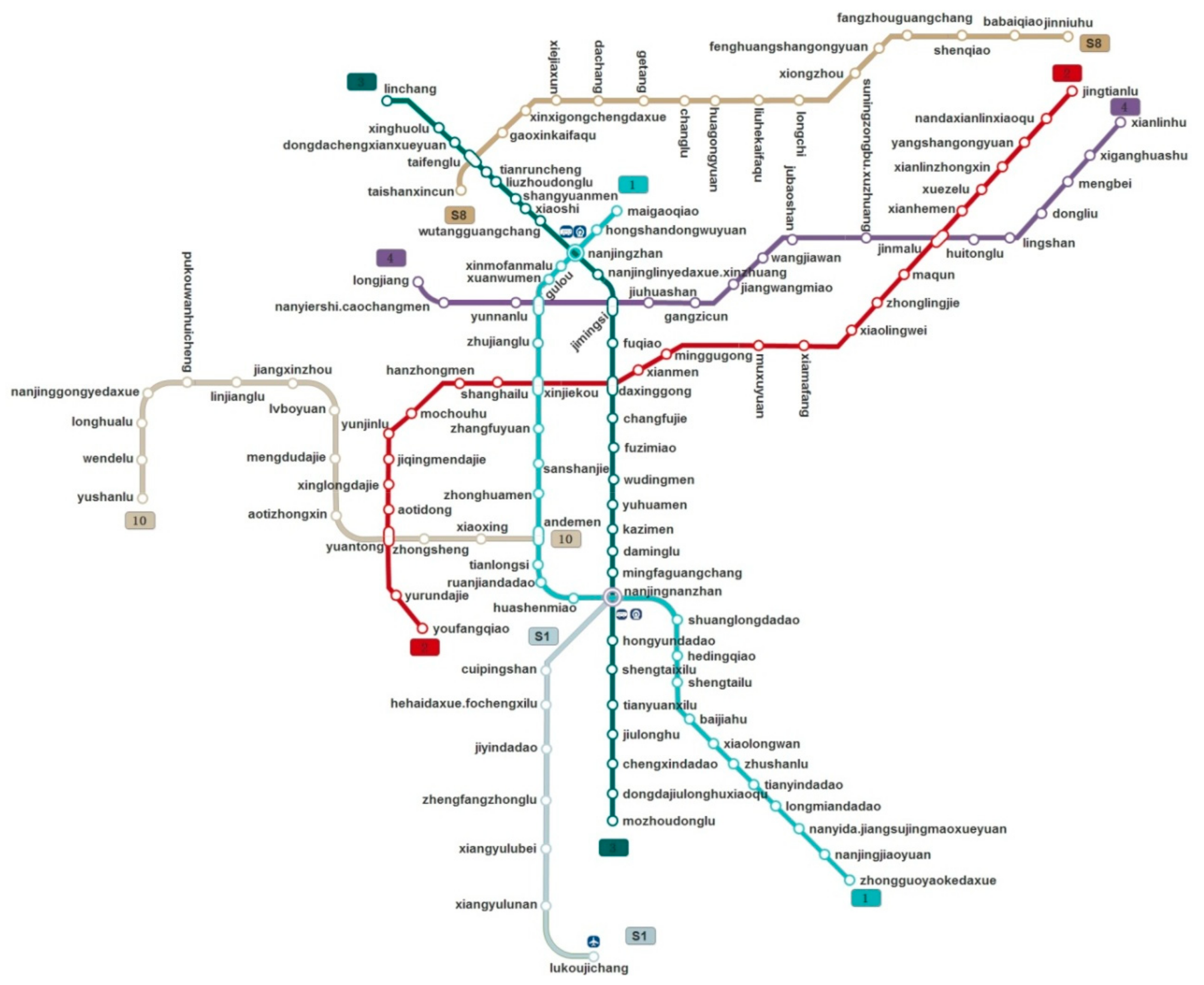
The rapid development of the Nanjing metro network and the universal application of smart cards provide the basis for the use of big data to analyze passenger behavior. Yang M investigated commuters using public bicycles to enter the subway, and analyzed personal characteristics and their experiences before and after going to work [45]. Based on the single line passenger flow data of Nanjing metro, Li J studied the influence of weather conditions on the passenger flow of Nanjing metro [46]. Zhao D analyzed the transfer situation between metro and public transport by using the data of the Nanjing bus smart card [47]. Wei Y analyzed the temporal and spatial change rule of passenger flow based on the data of the Nanjing metro smart card [48]. Wei Y used smart card data to propose the data filtering process and exception recognition, and classified and explained exceptions [49]. Yu J used the field data of the Nanjing metro stations to establish an improved social force model and simulate the efficiency of passengers under different organizational modes [50].
The existing research involves the OD records of various modes of transportation, and analyzes the occurrence preference, route selection, and destination demand of passengers. The model of the urban subway is established by using the complex network method, and the performance of the subway network is analyzed. Different from other modes of transportation, metro OD data have clear time records of entry and exit. As an important part of the comprehensive transportation system in large cities, the travel time of passengers has certain stability and regularity. How to set the appropriate index to analyze the OD data of the metro is an urgent problem to be solved in traffic information management.
Previous research includes the use of complex network methods to model the subway network and analyze its related performance. OD travel time, as an important indicator of passenger travel quality, is affected by various external factors. Traffic big data has been collected and analyzed in each subsystem. This provides an idea for this research, which can consider the complex performance index of the metro network and OD travel time index, and analyze their correlation. The smart card data of subway passengers will provide an accurate quantitative basis for correlation.
The development of traffic big data technology makes it possible to accurately evaluate and identify passengers’ travel behavior. In the urban public transportation system, the smart card has been widely used, especially in the subway and bus system. In addition, GPS is generally used to locate taxis, shared cars, and shared bicycles, which also provides the possibility to track the movement of passengers. But these data formats may face the situation of nonstandard format, which makes the analysis difficult. As an important part of the urban transportation system, the data of passengers’ swiping card is of typical significance. This study uses the swiping card records of subway passengers to evaluate the influencing factors of passenger travel time, which can lay a research foundation for refining the influencing factors in the future.
In this research, the card swiping data of the Nanjing metro smart card is used to select the five working days of passengers’ entry and exit records, establish an index evaluation system for the OD travel time of passengers, and select appropriate images to express the big data visually. This paper mainly adopts the complex network method to build the subway network model, and analyzes OD travel time with other indicators. The OD travel time index can be divided into three categories: time index, complex network index, and composite index. The Pearson correlation of these indexes of OD travel time was quantitatively analyzed. This will help to understand the factors affecting the travel time of passengers, improve the flow efficiency of passengers, and optimize the layout of the subway network and urban space.

2. Overview of Nanjing Metro and Analysis Process

2.1. Development of Nanjing Metro Lines

Table 1 shows the opening conditions of 7 metro lines in Nanjing at the beginning of 2017, including line name, opening time, number of stations, and length. From 2005 to 2017, Nanjing metro opened 7 metro lines in total. The time interval between the opening of line 1 and line 2 is relatively long. By 2014, line 10, S1, and S8 were opened continuously. Line 1 opened 16 stations in 2005, plus the South Extension Line opened in 2010, a total of 27 stations. Lines 1, 2, 3, and 4 form the main network of Nanjing metro. Line 10, S1, and S8 are extensions of the main line. Lines 1, 2, and 3 have a large number of stations. Except line 10, the length of other lines is more than 30 km. The long distance of extension line is caused by the large distance between stations.
Figure 1 shows the route map of Nanjing metro in 2017, with different colors to represent different routes. This metro line map is from the information released by Nanjing Metro Group Co., Ltd. [48]. The names of subway lines and stations are marked in the figure. From the subway figure, it can be seen that the main lines are 1, 2, 3, and 4, which run through the main urban area of Nanjing, and the intersection part constitutes the central area of Nanjing. The ring formed by the intersection of Line 1 and Line 3 forms the main urban area of Nanjing. The two intersections are the old railway station Nanjing Station and the new railway station Nanjing South Station, which are also important transportation hubs. Line 10, S1, and S8 are extension lines, connecting the remote suburbs of Nanjing. Xinjiekou station, the intersection of line 1 and line 2, is the geographical center and commercial center of Nanjing.
Table 2 shows the running direction, starting point, terminal point, and passing station of Nanjing metro lines. In the actual subway operation process, the subway is a two-way operation.

2.2. Smart Card Big Data of Nanjing Metro

According to the data released by Nanjing Municipal Bureau of Statistics, by the end of 2016, Nanjing had a permanent population of 8.27 million, including 6.78 million urban residents. The passenger flow data of Nanjing metro comes from the swiping card data of the passenger’s smart card, including card number, card type, station, time of entering and leaving the station, etc. The minimum unit of time data is seconds. More than one million OD records are generated by the AFC (Auto Fare Collection) system of Nanjing metro every day.

2.3. Correlation Analysis Process

Figure 2 shows the correlation analysis process of OD travel time indexes. Firstly, inappropriate data are filtered through data preprocessing. Then the OD travel time indexes can be divided into three categories: time index, complex network index, and composite index. Based on the complex network model, this research quantitatively analyzes the Pearson correlation of the indexes of OD travel time.

3. Data Preprocessing

Before analyzing the OD data of Nanjing metro, it is necessary to filter the data [32]. The abnormal data of OD includes the record of entering the station before yesterday, the record of entering the station after today, the record of negative use time, the record of more than 300 min, the record within one minute, and the record of entering and leaving the same station. The entry record before yesterday is that the passenger did not leave the station in time at that time, but chose to carry out remedial treatment afterwards on today.
The records of entering the station after today are usually concentrated in the early morning of the next day, which is a record error. The record with negative time does not conform to common sense, which is caused by the wrong record of the machine and equipment. According to the regulations of Nanjing metro, the maximum detention time of passengers in the metro network is 300 min. After this time, the smart card is locked and can no longer be used normally. According to the running time interval of the subway line, plus the time of passengers entering and leaving the station, the record within one minute is unreasonable. The entry and exit records of the same station are meaningless for the analysis of OD data.
Table 3 shows the data filtering of OD records in five working days, including the number before and after filtering every day, and the number filtered in each filtering step. As can be seen from Table 3, the total number of records ranges from 1.20 million to 1.32 million. The clear data number of each filtering step is relatively close, which reflects that these abnormal OD are common, so it is necessary to filter the data for further analysis.

4. Evaluation Indexes of OD Travel Time

OD travel time indexes can be divided into three categories: time index, complex network index, and composite index. Time index includes use time probability, passenger flow between stations, average time between stations, and time variance between stations. The complex network index is based on three complex networks, including the minimum number of rides between stations related to Space P model, and the shortest time between stations related to ride time model. Composite indicators include flow efficiency between stations and network flow efficiency.

4.1. Time Index

(1).
Use Time Probability
Formula 1 shows the calculating method of use time probability:
P i = T O D i i = 1 N T O D i
where P i is use time probability, i is the code of OD records, N is the total number of records, T O D i is the OD travel time of i .
Figure 3 shows the use time probability distribution in five days. It can be seen from the figure that the five-day curves are basically coincident, which shows that the use time probability distribution curve is relatively stable. The curve shows an obvious peak shape. The peak time is about 26 min, and the probability is more than 3%. The distribution of time used in 75–300 min is relatively flat, which shows that the time used is concentrated in 1–75 min, which may be detained in the subway network for some reason.
Figure 4 and Figure 5 show use time probability distribution of the early peak and late peak in five days, which can be compared with Figure 3. The early peak record selects the complete OD records from 7:00 to 9:00 of every morning. In the evening peak record, the complete OD records of the beginning and the end in the range of 17:00–19:00 every night are selected. The time is controlled within 120 min.
(2).
Passenger Flow between Stations
Passenger flow between stations refers to the traffic between different stations in a day. As of the beginning of 2017, there are 128 metro stations of Nanjing metro. Figure 6 shows the passenger flow distribution between stations on February 13. The figure is drawn with Origin software, and the contour module is used to represent different values with different colors. The distribution of the remaining four days is similar to this one.
It can be seen from Figure 5 that most of the traffic between stations is concentrated within 100, and a small part of the traffic is between 200 and 500, and some of the traffic is zero. Line 1, 2, and 3 are the main lines. The interaction between stations is frequent, and the flow is generally 200–500. Because the distance between extension lines is far, it is inconvenient to transfer, and the flow is zero. The flow between the same station of Line 1 and Line 2 is large, reaching 500–2000. The OD station with the largest flow is from Xingjiekou to Maigaoqiao, which exceeds 8000.
(3).
Average Time between Stations
Average time between stations refers to the average OD time between different stations in a day. Figure 7 shows the average time between stations on February 13. The distribution of the remaining four days is similar to this one. It can be seen from the figure that the average time between stations is mainly composed of 0–50 min and 50–100 min. Because of the relationship of zero traffic, there are zero records between stations. The average time between some stations is 100–150 min, and these records are mainly concentrated between 80–90 stations on Line 3.
Table 4 shows the five-day OD average time table, including the total number, the average time, the number of early peak, the average time of early peak, the number of late peak, and the average time of late peak. It can be seen from Table 4 that the average time of is basically stable at about 28 min, and the average time of early peak and late peak is kept at about 26 min. The number of early peak and late peak accounts for about 45% of the total number of days, but the time used is smaller than the average time of the whole day. This shows that the passenger flow during the peak period is larger, but the flow speed is faster. This may be the reason why the subway has opened more flights and the passengers are moving faster.
(4).
Time Variance between Stations
Time variance between stations indicates the deviation of a group of discrete data of time use between any two stations from the average time use between stations. This indicator reflects the difference of OD time of passenger flow between stations, as shown in Formula 2:
S i j 2 = 1 N 1 [ ( x i j 1 x i j ) 2 + ( x i j 2 x i j ) 2 + + ( x i j k x i j ) 2 + + ( x i j N x i j ) 2 ]
where S i j 2 is time variance between stations, and i , j are the station code, k is the number of OD records between stations, N is the total number of inter station records, and x i j = 1 N k = 1 N x k is the average value of inter station time.
Figure 8 shows time variance between stations on February 13. The distribution of the remaining four days is similar to this one. It can be seen from the figure that the time variance between stations mainly consists of two parts: 0–25, 25–50, and some are 50–100. On the whole, the time error is mainly concentrated in the OD alignment involving the station records of Line 1, 2, and 3, which is mainly due to the large passenger flow between these stations, resulting in the large time error of passengers.

4.2. Complex Network Index

Complex network index of Nanjing metro is closely related to OD time. The station codes are from the AFC of the Metro Management Department. The above Figure 1 and Table 2 show the station names and codes corresponding to different lines. When building the complex model of the Nanjing metro network, this research first uses MATLAB software to build the relationship matrix between Nanjing metro stations, and then uses the Netdraw module of UCINET software to import the relationship matrix, so as to draw the topological structure of Space P.
(1).
Space P Model and Minimum Number of Rides
Space P model regards subway stations as nodes. If there is a direct subway line between two stations, they establish a connection. Space P model reflects the transfer relationship between different metro lines. In order to facilitate analysis, the minimum number of rides between stations is used instead of the number of transfers. The number of rides between stations on the same metro line is 1. The number of rides can be presented by the shortest distance. The shortest distance between any two stations is the number of connections that the shortest path between two stations passes through. The shortest distance between stations represents the minimum number of rides between stations. Generally speaking, the more times passengers take the subway on different lines from the origination to the destination, it means that they need to travel farther and spend more time.
Figure 9 shows the Space P model of Nanjing metro network [39]. It can be clearly seen that the internal stations of the seven metro lines are closely connected, and there are important transport hubs between different metro lines, connecting the metro lines together.
Figure 10 shows the distribution of the minimum number of rides between stations. The minimum number of rides between stations is mainly 1, 2, and 3, which shows that the transfer between stations of Nanjing metro is relatively convenient. The number 1 is mainly distributed on the diagonal, because the stations of the same line are generally arranged in order. Because some stations are traffic hubs, the number of rides between the hubs and other stations is 1. The ride times between Line 1, 2, and 3 are basically 2, indicating that the transfer between main lines is relatively fast. The number 4 of rides is mainly concentrated in Line S8, which is too remote and inconvenient to interact with other lines, resulting in zero passenger flow of OD records.
(2).
Ride Time Model and Shortest Ride Time
Ride time means the actual time spent on the metro vehicle, not including inbound time, outbound time, and waiting time. Using the operation schedule of the train, the time interval between any adjacent stations is given to the contact value between stations, which constitutes the ride time model. This is a weighted directed network model. The directionality between stations is related to the direction of train operation. Figure 11 shows the up time interval of Nanjing metro, corresponding to the metro station sequence shown in Table 2. Figure 12 shows the down time interval of Nanjing metro. The time interval is simplified to minutes, which is the difference of departure time of adjacent stations.
According to the weighted network model, the shortest ride time between any two stations can be calculated. Figure 13 shows the shortest ride time distribution between stations. It can be seen from the figure that the shortest ride time between stations is mainly 0–20, 20–40, 40–60, 60–80. The time between stations on the diagonal is basically 0–20, because the stations are on the same line. The time between Line 1, 2, and 3 is less because of the connection of transportation hubs. The time between the station coded 70–80 and other stations reaches 80–120, because the station on Line S8 is inconvenient to transfer with other stations and takes a long time.

4.3. Composite Index

Composite index considers synthetically the time index and complex network index.
(1).
Flow Efficiency between Stations
The shortest ride time between any two stations is a stable value, which is only related to the train operation schedule. It is assumed that when passengers choose the route between two stations, the premise is to use the shortest ride time. Then, the waiting time between stations can be calculated. The waiting time here includes the time for passengers to enter, leave, and transfer. Here, time data between stations refers to the average value.
Formula 3 shows how to calculate the waiting time:
T w = T t T r
where T w is waiting time, T t is travel time, and T r is ride time.
Formula 4 shows the flow efficiency between stations:
E f = T r T t
where E f is flow efficiency between stations, T t is travel time, and T r is ride time.
Flow efficiency reflects the ratio of ride time to travel time. The higher the flow efficiency is, the better the network mobility is, and the shorter waiting time the passengers spend. Flow efficiency is directly proportional to ride time taken on the metro vehicle.
Figure 14 shows the flow efficiency distribution between stations on February 13. The distribution of the other four days is similar. As can be seen from the figure, the flow efficiency between stations is mainly composed of yellow, concentrated in 0.6–0.8. The value on the diagonal area is 0–0.2, which is due to the shorter time between stations on the same line. OD records involving remote routes show high flow efficiency, which indicates that waiting and transfer times between these stations are relatively smaller.
(2).
Network Flow Efficiency
Referring to the calculation method of flow efficiency between stations, network flow efficiency of Nanjing metro is calculated.
Table 5 shows the five-day network flow efficiency, including the average travel time, travel time variance, average waiting time, waiting time variance, and network flow efficiency.

5. Correlation Analysis

Before the correlation analysis of evaluation indexes of OD travel time, OD records with zero passenger flow must be removed first, otherwise the accuracy of the correlation analysis will be affected.
The purpose of correlation analysis is to understand the correlation between OD travel time and those factors, and the degree of correlation between them. The metro management department can promote the flow of passengers and improve the operation efficiency of the subway system by analyzing the influencing factors.

5.1. Pearson Correlation Model

The Pearson correlation model is generally used to measure the linear correlation between variables. When both variables are normal continuous variables and the relationship between them is linear, the Pearson correlation coefficient is used to show the correlation degree between the two variables.
The calculation formula is shown in Formula 5:
r = N x i y i x i y i N x i 2 ( x i ) 2 N y i 2 ( y i ) 2
where r is the correlation coefficient, i is the code of indicator value, x i and y i are the corresponding indicator values, N is the number of indicator values. In the actual calculation, two series are used to express different index values, and the correlation coefficient reflects the correlation between the two series.
The greater the absolute value of the correlation coefficient, the stronger the correlation. The closer the correlation coefficient is to 1 or −1, the stronger the correlation degree is. The closer the correlation coefficient is to 0, the weaker the correlation degree is. Generally, the following value ranges determine the correlation strength of variables: correlation coefficient 0.8–1.0 indicates extremely strong correlation, 0.6–0.8 indicates strong correlation, 0.4–0.6 indicates moderate correlation, 0.2–0.4 indicates weak correlation, and 0.0–0.2 indicates extremely weak correlation or no correlation.

5.2. Correlation Analysis of Travel Time between Stations

OD travel time of passengers includes inbound time, outbound time, transfer time, and ride time. The first three time factors can be unified as waiting time. The ride time is linearly related to the number of ride times. OD travel time is the sum of waiting time and taking time, which is a linear relationship with these two variables. The paper makes a supplementary explanation.
Table 6 shows the correlation between travel time, travel time variance and travel time, number of rides, and passenger flow between stations. Since the passenger’s ride time is based on the assumption of taking the minimum time, it is also necessary to analyze the correlation between ride time and travel time.
The parameters in the table refer to the relevant data between stations, travel time and the number of rides refers to the minimum value. It can be seen from the table that travel time is highly related to ride time, and travel time is strongly related to ride times, which means that the longer the ride time and the more rides, the longer the whole travel time. Passenger flow is negatively correlated with travel time. The larger the passenger flow is, the shorter the travel time is. The reason may be that when the number of passengers’ increases, the subway will be added, the moving speed of passengers will increase, and the average waiting time will be shorter.
Travel time variance is negatively correlated with travel time and passenger flow. The variance of travel time and the number of rides are sometimes a negative extremely weak correlation, sometimes a positive extremely weak correlation. This shows that the travel time variance has certain randomness and has no obvious correlation with other parameters.

5.3. Correlation Analysis of Waiting Time between Stations

Table 7 shows the correlation between the waiting time or waiting time variance and the number of rides, passenger flow. The waiting time is the difference between travel time and ride time. It can be seen from the table that the waiting time is strongly related to the number of rides. This shows that the more ride times it takes, the longer it takes to wait for the car, because the transfer of passengers takes more time. The weak correlation between waiting time and passenger flow is negative. This shows that the larger the passenger flow, the less waiting time. The reason may be that in the face of congestion, passengers are quicker. The waiting time variance is weakly correlated with the number of rides and the passenger flow, which indicates that the waiting time has a greater randomness.

5.4. Correlation Analysis of Flow Efficiency between Stations

Table 8 shows the correlation between the flow efficiency between stations and ride time, number of rides and passenger flow. The flow efficiency is positively correlated with ride time, which indicates that the longer the ride time is, the higher the flow efficiency is. This is because the ride time taken by metro has increased for the entire journey. The flow efficiency is weakly related to the number of passengers and the passenger flow, which has certain randomness.

6. Conclusions

From 2005 to 2017, Nanjing metro opened 7 metro lines in total. Lines 1, 2, 3, and 4 form the backbone network of Nanjing metro, with 128 stations in total. Nanjing metro’s AFC system accumulates the big data of passengers’ entering and leaving the station. These data can be used to analyze the temporal and spatial distribution of OD. However, to evaluate OD, we need to further establish systematic indexes and analyze the correlation of indexes.
Before analyzing the correlation, we select five working days of data to filter out the unreasonable data. OD time index can be divided into three categories: time, complex network, and composite index. The time index includes use time probability, passenger flow between stations, average use time between stations, and use time variance between stations. Space P and ride time models are constructed by the complex network method. The complex network index is based on three complex network models, including the minimum number of rides between stations related to Space P, and the shortest ride time between stations related to the ride time network model. Composite index includes flow efficiency between stations and network flow efficiency.
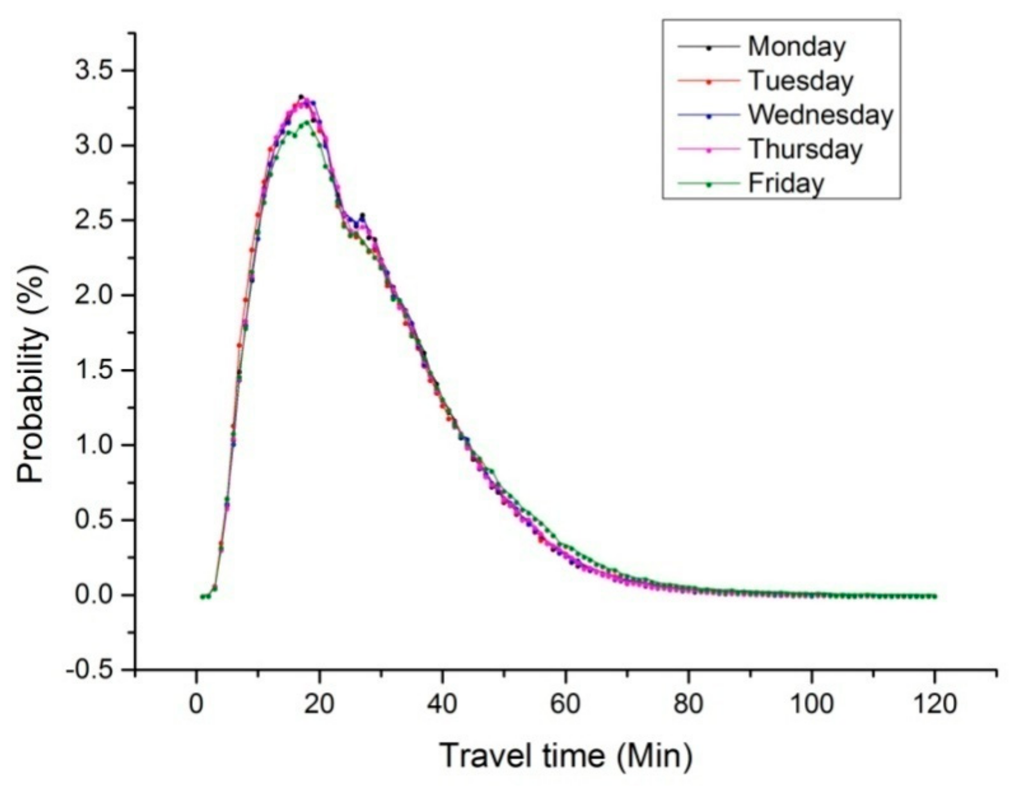
This research shows a five-day use time probability distribution. Taking February 13 as a representative, the distribution chart of time indexes is shown. The interaction between the main line stations is frequent and the traffic is large. The records of early peak and late peak account for about 45% of the total number of days. The average time between stations is mostly within 100 min. The main line has a large passenger flow between stations, which results in a relatively large time variance of passengers. The flow efficiency reflects the ratio of ride time to travel time. The higher the flow efficiency is, the better the network mobility is, and the shorter waiting time the passengers spend.
The Pearson correlation model is used to measure the linear correlation between the variables of the matrix, which is divided into positive correlation and negative correlation. The greater the absolute value of the correlation coefficient, the stronger the correlation.
Travel time is strongly related to ride time, and travel time is strongly related to ride times. This means that the longer the ride time and the more rides you take, the longer the travel time. The travel time variance has certain randomness, and has no obvious correlation with other indexes.
There is a strong correlation between waiting time and the number of rides. The weak correlation between waiting time and passenger flow is negative. The waiting time variance is weakly correlated with the number of rides and the passenger flow, which indicates that the waiting time has a greater randomness.
The flow efficiency is positively correlated with ride time, which indicates that the longer the ride time is, the higher the flow efficiency is. The flow efficiency is weakly related to the number of rides and the passenger flow, which has certain randomness.
Previous research considered the use of the complex network to model the subway network, analyzed various factors affecting OD travel time, and also used traffic big data as the basis for analysis. In this research, these methods are applied synthetically to analyze the influencing factors of OD travel time and the relationship between them. There is still some limitation in this research. Some abnormal travel records need to be further identified and filtered. Passenger’s travel route selection is based on the assumption of the shortest path, which needs to be combined with mobile signaling and other means for more accurate identification. Different stations, different weather, and different time periods have great influence on the travel time of passengers, which needs to be further analyzed in combination with previous research.
Based on the big data of the Nanjing metro smart card, this study uses the complex network method to construct and analyze the OD travel time index. These indexes consider the connection between the starting point and the terminal point of passengers, and can be used for quantitative evaluation of the connection between the subway station and the network. This method can be extended to the bus system and public bicycle system. Future research can further increase the length of the observation date, select subway data from different cities, carefully distinguish the influencing factors of passenger travel time, and analyze their correlation, so as to control variables and improve the operation efficiency and management level of the transportation system.

Author Contributions

W.T. undertook the data collection. C.J. provided an interpretation of the results. Y.X. and Y.W. wrote the majority of the paper. Y.X. contributed to the paper review and editing. All authors have read and agreed to the published version of the manuscript.

Funding

This research was funded by Natural Science Foundation of Zhejiang Province (No.LY20E080011), Key Project of National Natural Science Foundation of China (No. 51638004), Basic Research Program of Science and Technology Commission Foundation of Jiangsu Province (No. BK20180775), National Natural Science Foundation of China (No. 71701099).

Acknowledgments

The authors would like to express their sincere thanks to the anonymous reviewers for their constructive comments on an earlier version of this manuscript.

Conflicts of Interest

The authors declare no conflict of interest.

References

  1. Kim, H.; Nam, D.; Suh, W.; Cheon, S.H. Origin-destination trip table estimation based on subarea network OD flow and vehicle trajectory data. Transp. Plan. Technol. 2018, 41, 265–285. [Google Scholar] [CrossRef]
  2. Kim, K.; Kim, V.; Kim, H. Spatiotemporal auto-regressive model for origin–destination air passenger flows. J. R. Stat. Soc. Ser. A 2019, 182, 1003–1016. [Google Scholar] [CrossRef]
  3. Zhang, C.; Wang, J.; Lai, J.; Yang, X.; Su, Y.; Dong, Z. Extracting origin-destination with vehicle trajectory data and applying to coordinated ramp metering. J. Adv. Transp. 2019, 8, 8469316. [Google Scholar] [CrossRef] [Green Version]
  4. Liu, L.; Qiu, Z.; Li, G.; Wang, Q.; Ouyang, W.; Lin, L. Contextualized spatial-temporal network for taxi origin-destination demand prediction. Ieee Trans. Intell. Transp. Syst. 2019, 20, 3875–3887. [Google Scholar] [CrossRef] [Green Version]
  5. Bachir, D.; Khodabandelou, G.; Gauthier, V.; El Yacoubi, M.; Puchinger, J. Inferring dynamic origin-destination flows by transport mode using mobile phone data. Transp. Res. Part C Emerg. Technol. 2019, 101, 254–275. [Google Scholar] [CrossRef] [Green Version]
  6. Bachir, D.; Khodabandelou, G.; Gauthier, V.; El Yacoubi, M.; Puchinger, J. Constructing time-dependent origin-destination matrices with adaptive Zoning scheme and measuring their similarities with taxi trajectory data. IEEE Access 2019, 7, 77723–77737. [Google Scholar]
  7. Javani, B.; Babazadeh, A. Origin-destination-based truncated quadratic programming algorithm for traffic assignment problem. Transp. Lett. Int. J. Transp. Res. 2016, 9, 166–176. [Google Scholar] [CrossRef]
  8. Mehrabipour, M.; Hajibabai, L.; Hajbabaie, A. A decomposition scheme for parallelization of system optimal dynamic traffic assignment on urban networks with multiple origins and destinations. Comput. Aided Civ. Infrastruct. Eng. 2019, 34, 915–931. [Google Scholar] [CrossRef]
  9. Hoang, N.H.; Vu, H.L.; Panda, M.; Lo, H.K. A linear framework for dynamic user equilibrium traffic assignment in a single origin-destination capacitated network. Transp. Res. Part B Methodol. 2019, 126, 329–352. [Google Scholar] [CrossRef]
  10. Wang, Y.; Ma, X.; Liu, Y.; Gong, K.; Henricakson, K.C.; Xu, M.; Wang, Y. A two-stage algorithm for origin-destination matrices estimation considering dynamic dispersion parameter for route choice. PLoS ONE 2016, 11, e0146850. [Google Scholar]
  11. Li, D.; Miwa, T.; Xu, C.; Li, Z. Non-linear fixed and multi-level random effects of origin-destination specific attributes on route choice behavior. Iet Intell. Transp. Syst. 2019, 13, 654–660. [Google Scholar] [CrossRef]
  12. Ou, J.; Lu, J.; Xia, J.; An, C.; Lu, Z. Learn, assign and search: Real-time estimation of dynamic origin-destination flows using machine learning algorithms. IEEE Access 2019, 7, 26967–26983. [Google Scholar] [CrossRef]
  13. Duan, Z.; Zhang, K.; Chen, Z.; Liu, Z.; Tang, L.; Yang, Y.; Ni, Y. Prediction of city-scale dynamic taxi origin-destination flows using a hybrid deep neural network combined with travel time. IEEE Access 2019, 7, 127816–127832. [Google Scholar] [CrossRef]
  14. Yang, S.; An, C.; Wu, Y.J.; Xia, J. Origin-destination-based travel time reliability. Transp. Res. Rec. J. Transp. Res. Board 2017, 2643, 139–159. [Google Scholar] [CrossRef]
  15. Margaretic, P.; Thomas-Agnan, C.; Doucet, R. Spatial dependence in (origin-destination) air passenger flows. Pap. Reg. Sci. 2017, 96, 357–380. [Google Scholar] [CrossRef] [Green Version]
  16. Hanseler, F.S.; Molyneaux, N.A.; Bierlaire, M. Estimation of pedestrian origin-destination demand in train stations. Transp. Sci. 2017, 51, 981–997. [Google Scholar] [CrossRef] [Green Version]
  17. Nigro, M.; Cipriani, E.; Giudice, A. Exploiting floating car data for time-dependent Origin-Destination matrices estimation. J. Intell. Transp. Syst. 2017, 22, 159–174. [Google Scholar] [CrossRef]
  18. Ma, W.; Qian, Z. Statistical inference of probabilistic origin-destination demand using day-to-day traffic data. Transp. Res. Part C Emerg. Technol. 2018, 88, 227–256. [Google Scholar] [CrossRef] [Green Version]
  19. Dai, X.; Sun, L.; Xu, Y. Short-term origin-destination based metro flow prediction with probabilistic model selection approach. J. Adv. Transp. 2018, 2018, 5942763. [Google Scholar] [CrossRef]
  20. Wang, J.; Deng, W.; Guo, Y. New bayesian combination method for short-term traffic flow forecasting. Transp. Res. Part C Emerg. Technol. 2014, 43, 79–94. [Google Scholar] [CrossRef]
  21. Zhu, S.; Zheng, H.; Peeta, S.; Guo, Y.; Cheng, L.; Sun, W. Optimal heterogeneous sensor deployment strategy for dynamic origin-destination demand estimation. Transp. Res. Rec. J. Transp. Res. Board 2016, 2567, 18–27. [Google Scholar] [CrossRef]
  22. Zhu, N.; Ma, S.; Zheng, L. Travel time estimation oriented freeway sensor placement problem considering sensor failure. J. Intell. Transp. Syst. 2017, 1, 26–40. [Google Scholar] [CrossRef]
  23. Hobson, B.; Lowcay, D.; Gunay, H.B. Opportunistic occupancy-count estimation using sensor fusion: A case study. Build. Env. 2019, 159, 1061154. [Google Scholar] [CrossRef]
  24. Moslem, S.; Ghorbanzadeh, O.; Blaschke, T.; Duleba, S. Analysing stakeholder consensus for a sustainable transport development decision by the fuzzy AHP and interval AHP. Sustainability 2019, 11, 3271. [Google Scholar] [CrossRef] [Green Version]
  25. Ghorbanzadeh, O.; Moslem, S.; Blaschke, T.; Duleba, S. Sustainable urban transport planning considering different stakeholder groups by an interval-AHP decision support model. Sustainability 2019, 11, 9. [Google Scholar] [CrossRef] [Green Version]
  26. Duleba, S.; Moslem, S. Sustainable urban transport development with stakeholder participation, an AHP-Kendall model: A case study for Mersin. Sustainability 2018, 10, 3647. [Google Scholar] [CrossRef] [Green Version]
  27. Duleba, S.; Moslem, S. Examining Pareto optimality in analytic hierarchy process on real Data: An application in public transport service development. Expert Syst. Appl. 2019, 116, 21–30. [Google Scholar] [CrossRef]
  28. Moslem, S.; Duleba, S. Sustainable urban transport development by applying a Fuzzy-AHP model: A case study from Mersin, Turkey. Urban Sci. 2019, 3, 55. [Google Scholar] [CrossRef] [Green Version]
  29. Jiang, X.; Wang, H.; Guo, X.; Gong, X. Using the FAHP, ISM, and MICMAC approaches to study the sustainability influencing factors of the last mile delivery of rural E-commerce logistics. Sustainability 2019, 11, 3937. [Google Scholar] [CrossRef] [Green Version]
  30. Guo, Y.; Wang, J.; Peeta, S. Impacts of internal migration, household registration system, and family planning policy on travel mode choice in China. Travel Behav. Soc. 2018, 13, 128–143. [Google Scholar] [CrossRef]
  31. Ruan, Y.; Zhu, D.; Lu, J. Social adaptation and adaptation pressure among the “drifting elderly” in China: A qualitative study in Shanghai. Int. J. Health Plan. Manag. 2019, 34, 1149–1165. [Google Scholar] [CrossRef]
  32. Guo, Y.; Peeta, S. Impacts of personalized accessibility information on residential location choice and travel behavior. Travel Behav. Soc. 2020, 19, 99–111. [Google Scholar] [CrossRef]
  33. Li, Y.; Guo, Y.; Lu, J.; Peeta, S. Impacts of congestion pricing and reward strategies on automobile travelers’ morning commute mode shift decisions. Transp. Res. Part A Policy Pr. 2019, 125, 72–88. [Google Scholar] [CrossRef]
  34. Wang, D.; Lin, T. Built environment, travel behavior, and residential self-selection: A study based on panel data from Beijing, China. Transportation 2019, 46, 51–74. [Google Scholar] [CrossRef]
  35. Cheng, G.; Zhao, S.; Li, J. The effects of latent attitudinal variables and sociodemographic differences on travel behavior in two small, underdeveloped cities in China. Sustainability 2019, 11, 1306. [Google Scholar] [CrossRef] [Green Version]
  36. Guo, Y.; Wang, J.; Peeta, S.; Anastasopoulos, P.C. Personal and societal impacts of motorcycle ban policy on motorcyclists’ home-to-work morning commute in China. Travel Behav. Soc. 2020, 19, 137–150. [Google Scholar] [CrossRef]
  37. Feng, J.; Li, X.; Mao, B.; Xu, Q.; Bai, Y. Weighted complex network analysis of the different patterns of metro traffic flows on weekday and weekend. Discret. Dyn. Nat. Soc. 2016, 2016, 9865230. [Google Scholar] [CrossRef]
  38. Saberi, M.; Mahmassani, H.S.; Brockmann, D.; Hosseini, A. A complex network perspective for characterizing urban travel demand patterns: Graph theoretical analysis of large-scale origin-destination demand networks. Transportation 2017, 44, 1383–1402. [Google Scholar] [CrossRef]
  39. Zhang, J.; Wang, S.; Wang, X. Comparison analysis on vulnerability of metro networks based on complex network. Phys. A Stat. Mech. Its Appl. 2019, 496, 72–78. [Google Scholar] [CrossRef]
  40. Wu, X.; Dong, H.; Tse, C.K.; Ho, I.W.; Lau, F.C. Analysis of metro network performance from a complex network perspective. Phys. A Stat. Mech. Its Appl. 2018, 492, 553–563. [Google Scholar] [CrossRef]
  41. Wei, Y.; Ning, S. Establishment and analysis of the supernetwork model for Nanjing metro transportation system. Complexity 2018, 2018, 4860531. [Google Scholar] [CrossRef]
  42. Yu, W.; Chen, J.; Yan, X. Space-time evolution analysis of the Nanjing metro network based on a complex network. Sustainability 2019, 11, 523. [Google Scholar] [CrossRef] [Green Version]
  43. Yu, W.; Wang, T.; Zheng, Y.; Chen, J. Parameter Selection and Evaluation of Robustness of Nanjing Metro Network Based on Supernetwork. IEEE Access 2019, 7, 70876–70890. [Google Scholar] [CrossRef]
  44. Kanwar, K.; Kumar, H.; Kaushal, S. Complex network based comparative analysis of Delhi Metro network and its extension. Phys. A Stat. Mech. Its Appl. 2019, 526, 120991. [Google Scholar] [CrossRef]
  45. Yang, M.; Liu, X.; Wang, W.; Li, Z.; Zhao, J. Empirical analysis of a mode shift to using public bicycles to access the suburban metro: Survey of Nanjing, China. J. Urban Plan. Dev. 2016, 12, 05015011. [Google Scholar] [CrossRef]
  46. Li, J.; Li, X.; Chen, D.; Godding, L. Assessment of metro ridership fluctuation caused by weather conditions in Asian context: Using archived weather and ridership data in Nanjing. J. Transp. Geogr. 2018, 66, 356–368. [Google Scholar] [CrossRef]
  47. Zhao, D.; Wang, W.; Li, C.; Ji, Y.; Hu, X.; Wang, W. Recognizing metro-bus transfers from smart card data. Transp. Plan. Technol. 2019, 42, 70–83. [Google Scholar] [CrossRef]
  48. Yu, W.; Bai, H.; Chen, J.; Yan, X. Analysis of space-time variation of passenger flow and commuting characteristics of residents using smart card data of Nanjing metro. Sustainability 2019, 11, 4989. [Google Scholar] [CrossRef] [Green Version]
  49. Yu, W.; Bai, H.; Chen, J.; Yan, X. Anomaly detection of passenger OD on Nanjing metro based on smart card big data. IEEE Access 2019, 7, 138624–138636. [Google Scholar] [CrossRef]
  50. Yu, J.; Ji, Y.; Gao, L.; Gao, Q. Optimization of metro passenger organizing of alighting and boarding processes: Simulated evidence from the metro station in Nanjing, China. Sustainability 2019, 11, 3682. [Google Scholar] [CrossRef] [Green Version]
Figure 1. Nanjing metro line map.
Sustainability 12 01113 g001
Figure 2. Correlation analysis process.
Sustainability 12 01113 g002
Figure 3. Use time probability distribution in five days.
Sustainability 12 01113 g003
Figure 4. Use time probability distribution in early peak of five days.
Sustainability 12 01113 g004
Figure 5. Use time probability distribution in evening peak of five days.
Sustainability 12 01113 g005
Figure 6. Passenger flow distribution between stations on February 13.
Sustainability 12 01113 g006
Figure 7. Average time between stations on February 13.
Sustainability 12 01113 g007
Figure 8. Time variance between stations on February 13.
Sustainability 12 01113 g008
Figure 9. Space P model of Nanjing metro.
Sustainability 12 01113 g009
Figure 10. Distribution of the minimum number of rides between stations.
Sustainability 12 01113 g010
Figure 11. Up time interval of Nanjing metro.
Sustainability 12 01113 g011
Figure 12. Down time interval of Nanjing Metro.
Sustainability 12 01113 g012
Figure 13. Distribution of the shortest ride time between stations.
Sustainability 12 01113 g013
Figure 14. Flow efficiency distribution between stations on February 13.
Sustainability 12 01113 g014
Table 1. Opening sequence of Nanjing metro lines.
Opening SequenceNumber of StationsLength (km)Opening Year
127(16)38.92005
22637.92010
101421.62014
S1837.32014
S81745.22014
32944.92015
41833.82017
Table 2. Direction and stations of Nanjing metro lines.
Line CodeOriginationDestinationStation Code
1maigaoqiaozhongguoyaokedaxue[16, 15, 14, 13, 12, 11, 10, 9, 8, 7, 6, 5, 41, 42, 43, 44, 45, 46, 47, 48, 49, 50, 51, 52, 53, 54, 55]
2jingtianluyoufangqiao[40, 39, 38, 37, 36, 35, 34, 33, 32, 31, 30, 29, 28, 27, 26, 9, 25, 24, 23, 22, 21, 20, 19, 2, 18, 17]
3linchangmouzhoudonglu[89, 90, 91, 73, 92, 93, 94, 95, 96, 14, 97, 98, 99, 26, 100, 101, 102, 103, 104, 105, 106, 44, 107, 108, 109, 110, 111, 112, 113]
4xianlinhulongjiang[128, 127, 126, 125, 124, 123, 34, 122, 121, 120, 119, 118, 117, 98, 11, 116, 115, 114
10yushanluandemen[64, 63, 62, 61, 60, 59, 58, 57, 56, 1, 2, 3, 4, 5]
S1nanjingnanzhanlukoujichang[44, 71, 70, 69, 68, 67, 66, 65]
S8jinniuhutaishanxincun[88, 87, 86, 85, 84, 83, 82, 81, 80, 79, 78, 77, 76, 75, 74, 73, 72]
Table 3. Data filtering of OD (origination–destination) records in five working days.
DateWeekWhole NumberNumber After FilteringInbound Before YesterdayInbound After TodayNegative
Use Time
More than 300 min0-1minInbound and Outbound on Same Stations
2.13Monday1,228,1311,218,423932915124018866445
2.14Tuesday1,305,5211,294,9481764410131520127016
2.15Wednesday1,240,3081,229,7042482512129521376887
2.16Thursday1,201,7131,192,083682811131119996213
2.17Friday1,324,3421,313,34072286131321197464
Table 4. OD average time in five days.
DateWhole NumberAverage Time
(min)
Number of Early PeakAverage Time of Early Peak (min)Number of Evening PeakAverage Time of Evening Peak (min)
2.131,218,42328.41275,28426.62292,46626.51
2.141,294,94828.13270,29126.26322,73626.37
2.151,229,70428.61271,89926.93293,06226.60
2.161,192,08328.31265,42726.28286,64826.59
2.171,313,34029.00268,91526.58320,66427.42
Table 5. Network flow efficiency in five days.
DateWhole NumberAverage Travel Time (min)Travel Time VarianceAverage Waiting Time (min)Waiting Time VarianceNetwork Flow Efficiency
2.131,218,42328.41285.418.8959.260.6871
2.141,294,94828.13283.479.0162.030.6797
2.151,229,70428.61290.609.1264.150.6812
2.161,192,08328.31280.058.8856.820.6863
2.171,313,34029.00305.179.3063.600.6793
Table 6. Correlation analysis of travel time between stations.
Travel TimeTravel Time Variance
DateRide TimeNumber of RidesPassenger FlowRide TimeNumber of RidesPassenger Flow
2.130.96540.6374−0.3147−0.0196−0.0034−0.0234
2.140.96570.6438−0.3066−0.01960.0146−0.0217
2.150.96370.6437−0.3220−0.01820.0039−0.0303
2.160.96330.6345−0.3162−0.00730.0128−0.0278
2.170.96650.6431−0.3163−0.0131−0.0049−0.0290
Table 7. Correlation analysis of waiting time between stations.
Waiting TimeWaiting Time Variance
DateNumber of RidesPassenger FlowNumber of RidesPassenger Flow
2.130.6386−0.2630−0.0034−0.0234
2.140.6573−0.25660.0146−0.0217
2.150.6523−0.27810.0039−0.0303
2.160.6249−0.26040.0128−0.0278
2.170.6517−0.2690−0.0049−0.0290
Table 8. Correlation analysis of flow efficiency between stations.
Flow Efficiency
DateRide TimeNumber of RidesPassenger Flow
2.130.64810.0752−0.1007
2.140.64600.0714−0.1096
2.150.64420.0695−0.0873
2.160.64840.0716−0.1013
2.170.64720.0774−0.1115

