A Multi-commodity Network Flow Model for Sustainable Performance Evaluation in City Logistics: Application to the Distribution of Multi-tenant Buildings in Tokyo

Abstract

The distribution of goods in crowded city centers is a major challenge. In this paper, we propose a methodology for evaluating the performance of a parcel distribution network in city logistics. This methodology encompasses the main entities of a two-tier distribution system made up of carriers, huge shopping centers (multi-tenant buildings) and intermediate depots (urban consolidation centers), as well as the parcel flows between them. This methodology aims to optimize the transport flows (distance traveled) of a given distribution network while also quantifying the impact in terms of sustainable development by measuring gas emissions. Two different states of the network with different connectivity degrees are evaluated and compared: the current state of the network as well as its future state. The transport network modeling is based on a network flow, which is expressed in linear programming and implemented with an optimization solver. The validation of this methodology is based on the parcel distribution of the Multi-tenant Buildings of the city of Tokyo. The findings are that the network with greater connectivity between the entities brings significant traveled distance reduction as well as a reduction of emissions of CO2. Another finding is that the grouping of the parcels (i.e., pooling) brings a reduction of the distance traveled compared to the transport organization without grouping and contributes to a reduction in the number of trucks.

1. Introduction

City logistics aims at optimizing logistics activities in urban areas with the support of advanced information and communication technologies towards sustainable development [1,2]. Our study deals with the transport flow analysis in the context of the last-mile delivery. Even if the last mile represents a small part of the whole transportation chain, it is known to represent a significant part (about one-third) of the total transportation costs [3]. This problem generates traffic jams as well as an increase in air and noise pollution; it has a strong impact on the quality of life in cities and consequently undermines the objectives of sustainable development.

In this article, we focus on the distribution of goods from the outskirts of the city to the main buildings located in the city center of a megalopolis. In this context, two-tier distribution systems have emerged for many years; therefore, the main components of the distribution networks studied in this paper are as follows:

• The multi-tenant buildings (MTB) are shopping complexes containing hundreds of shops, restaurants, offices, open spaces, and even sometimes a theater. These buildings with high population densities are the place of complex relationships between the owners, the tenants, and the management companies from which multiple problems can emerge. Let us mention, for instance, sustainable development problems such as energy consumption [4], and organizational problems such as regulating flows between different stakeholders. In this article, we focus precisely on the distribution flows of parcels to these buildings.
• The urban consolidation center (UCC) is a way to consolidate the flow of deliveries in the last mile [5]. UCCs are central elements in vertical collaboration that make it possible to group parcels that have been addressed for certain customers in a single flow. These centers facilitate last-mile delivery by providing equipment that allows large vehicles to enter these spaces and consolidating the flows that can be formatted to suit the delivery mode more adapted to the last mile.
• The carriers (CRRs) are independent companies that receive transport orders from the suppliers of the final customers located in the MTBs. They deliver parcels from their depot to a given final destination (i.e., MTB) and use intermediate logistics platforms such as UCC to optimize their own transport performance.

This paper aims at modeling and optimizing freight flows in order to compare the performances of different distribution networks. The measured performances cover traditional indicators such as distance and number of vehicles, but they also include indicators related to greenhouse gases and particulate emissions that are important in terms of sustainable development. The main objective of this paper is to highlight the interest of an open distribution network where the infrastructure can be shared by different transport operators. The following sections present a literature review, define the problem and working hypothesis, and present a linear programming model to optimize flows. Lastly, we report the experiments carried out for the freight distribution in Tokyo. A conclusion ends the paper.

2. Literature Review

Most of the work in transport planning involves the development of demand forecasting models coupled with network models to analyze distribution flows. For instance, [6] proposed an Origin–Destination synthesis model for a multi-commodity transport system. A commodity corresponds to a good (or a parcel) that has to be transported from a source node to a destination node. Our contribution also concerns the multi-commodity context, focusing on analyzing the distribution flows.

Research in the field of distribution in urban logistics is mainly oriented towards the design of distribution networks. The so-called Service Network design term is extensively used to refer to many design planning problems in transportation and distribution systems [7,8] proposed a low carbon network planning model for a city logistic distribution system; their model aims to decide opening distribution centers, and the objective function integrates operational costs with or without tax carbon for comparison purposes. [9] proposed to select among four kinds of typical distribution modes: self-distribution mode, mutual distribution mode, third party distribution mode, and common distribution mode while also reducing the carbon emissions. [10] presented a mathematical model to build a green distribution system minimizing the total cost made up of economic cost, environmental cost, and socioeconomic cost. The focus of our study is similar to the two-tier city logistics network proposed by [11]; however, ours is more close to the real-life case as the base network of freight carriers’ depots, urban consolidation centers, and multi-tenant buildings already exists (for example, the Tokyo case study presented later in the paper). We propose a complete integration and analyze the performance of these existing (real-life) networks with and without complete integration.

At the core of the studied network are the urban consolidation centers. There are several studies [12,13] addressing advantages of collaboration in the form of reducing the negative impact of urban transport. For example, [14] used a multi-agent simulation in cases of urban goods delivery using urban consolidation centers and evaluated the system based on the multiple criteria including reducing delivery costs and CO2, NOx, and suspended particulate matter (SPM) emissions. [15] also reported similar advantages (reduced number of tours needed to meet the customer’s demands and decreased the required distance) in a simulation to evaluate a UCC for distribution in Athens. This challenging topic has been reviewed in depth in [16]. The authors distinguished between vertical collaboration, which relies on breaking down transportation routes into multiple tiers, and horizontal collaboration, focusing on the question of centralized versus decentralized transportation planning. In this paper, we focus on vertical collaboration using UCCs in the last-mile delivery.

Apart from any studies which have reported the role and the potential impact of UCC on reducing nuisance [17,18,19,20,21,22,23], some real-life pilot projects implementing UCCs have also been reported [24,25]. For example, [26] reported a new type of urban consolidation center (Binnenstadservice.nl) in Nijmegen, which became successful by focusing on receivers rather than on carriers. On the other hand, the mixed success of the UCCs is reported due to several obstacles such as an increase of overall cost or space limitation in the city center. The analysis of the reasons for the failures or successes of UCCs is beyond the scope of this article and can be found in [27]. The recent review of UCC literature proposed by [28] highlights important findings, including the following three points: (i) many studies relate to the optimization of potential initiatives, but very few focus on existing initiatives; (ii) very few studies are oriented towards the overall impact of the UCCs on the distribution system; (iii) few studies measure or assess their environmental impact. Our contribution addresses some of these shortcomings. Indeed, we focus on the one hand on the whole network that includes the UCCs and that covers several entities of the distribution chain, and on the other hand, we carry out an analysis at the sustainable level of an existing and operating network in the city of Tokyo.

In order to assess the impact of distribution networks implementing UCCs in the centers of large cities, we chose to model the distribution of parcels from carriers to MTBs as a multi-commodity network flow (MCNF) problem.

An exhaustive review of the MCNF is beyond the scope of this article, and readers can refer to [29] for a comprehensive study of commodity flow models. The MCNF can be solved in polynomial time using linear programming if the flows are real values. However, the MCNF is an NP-hard problem if the flows are integers so it remains a difficult problem to solve [30]. Many formulations and many solution methods have been proposed to solve this problem using advanced mathematical programming approaches [31]. For instance, [32] presented a branch and price and cut algorithm to solve integers MCNF. The MCNF has been used in many domains such as telecommunication, production planning, logistics, and transportation. Regarding transportation, let us mention for instance a less than truckload (LTL) transportation problem which has been formulated as an MCNF in [33] and [34]. In our study, the overall objective is to ship the commodities through the network at the lowest possible cost while satisfying the arc capacities; furthermore, the carriers have to consolidate shipments in order to minimize the total time. To our knowledge, there is no work using a multi-commodity network flow model to assess the transportation flows in city logistics in the context of distribution of multi-tenant buildings. The model described in the next section is an extension of the integral MCNF, oriented towards the calculation of the flow of trucks into the network.

3. Materials and Methods

Our objective is to evaluate the performance of a parcel distribution network in terms of emissions and distance traveled. Our methodology can be described in the following three steps, corresponding to the next three sub-sections:

• First we set out the working hypotheses in order to define the studied problem (Section 3.1). In this section, two key definitions are introduced: one characterizes the degree of connectivity of a distribution network (labeled as “integration”); the second concerns the grouping level of the flow of transported parcels (labeled as “pooling”).
• Next, we propose a model of the distribution network in linear programming (Section 3.2).
• Last, we address the present the experimental framework in order to validate our solution approach based on an example case in Tokyo (Section 3.3).

3.1. Problem Definition and Hypothesis

The first key definition relates to the degree of connectivity of the network used by different partners. We have considered two distribution networks in this study, depending on the degree of accessibility of the urban consolidation centers and the level of connectivity of transportation infrastructure:

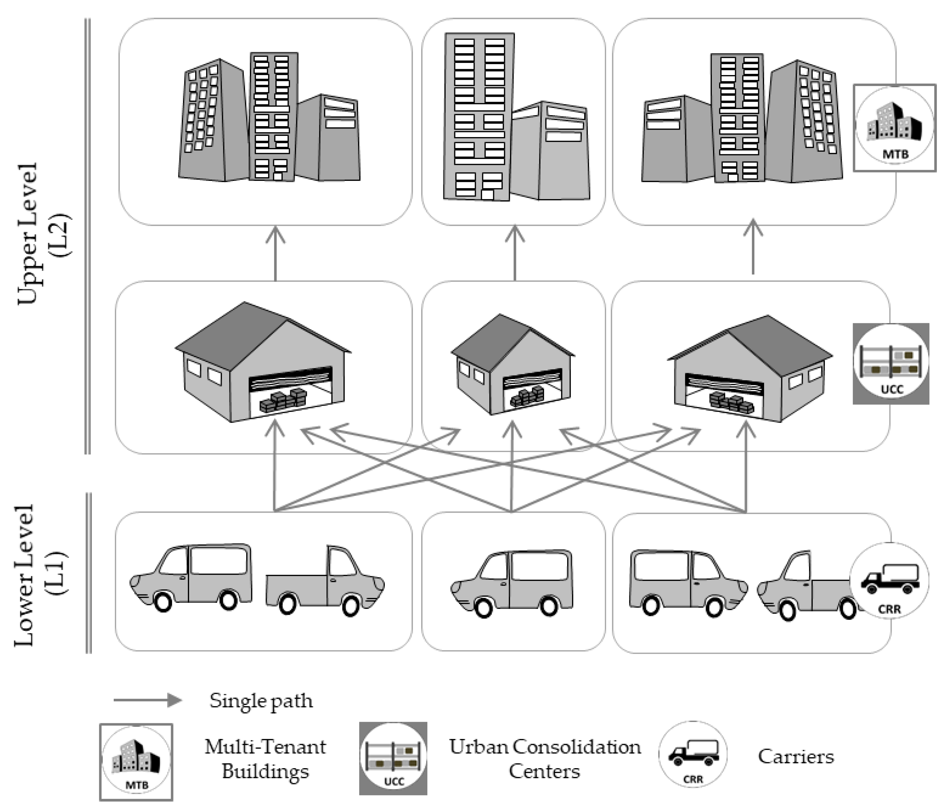
• The first distribution network is made up of UCCs, which are owned by transportation companies. Each facility is used by a unique owner; the service and space are not shared with other companies. In this case, UCCs are operated independently of each other, without any integration between different transport partners. Each UCC is dedicated to the deliveries to one or more consumers’ locations in a specific multi-tenant building. In this configuration, only a single path exists from a carrier to an MTB with no alternative solution. Figure 1 represents a simplified case containing three MTBs, three UCCs, and three carriers with their own distribution chain. As there is no connectivity (integration) between UCCs, this network configuration is labeled as NI (i.e., No Integration).
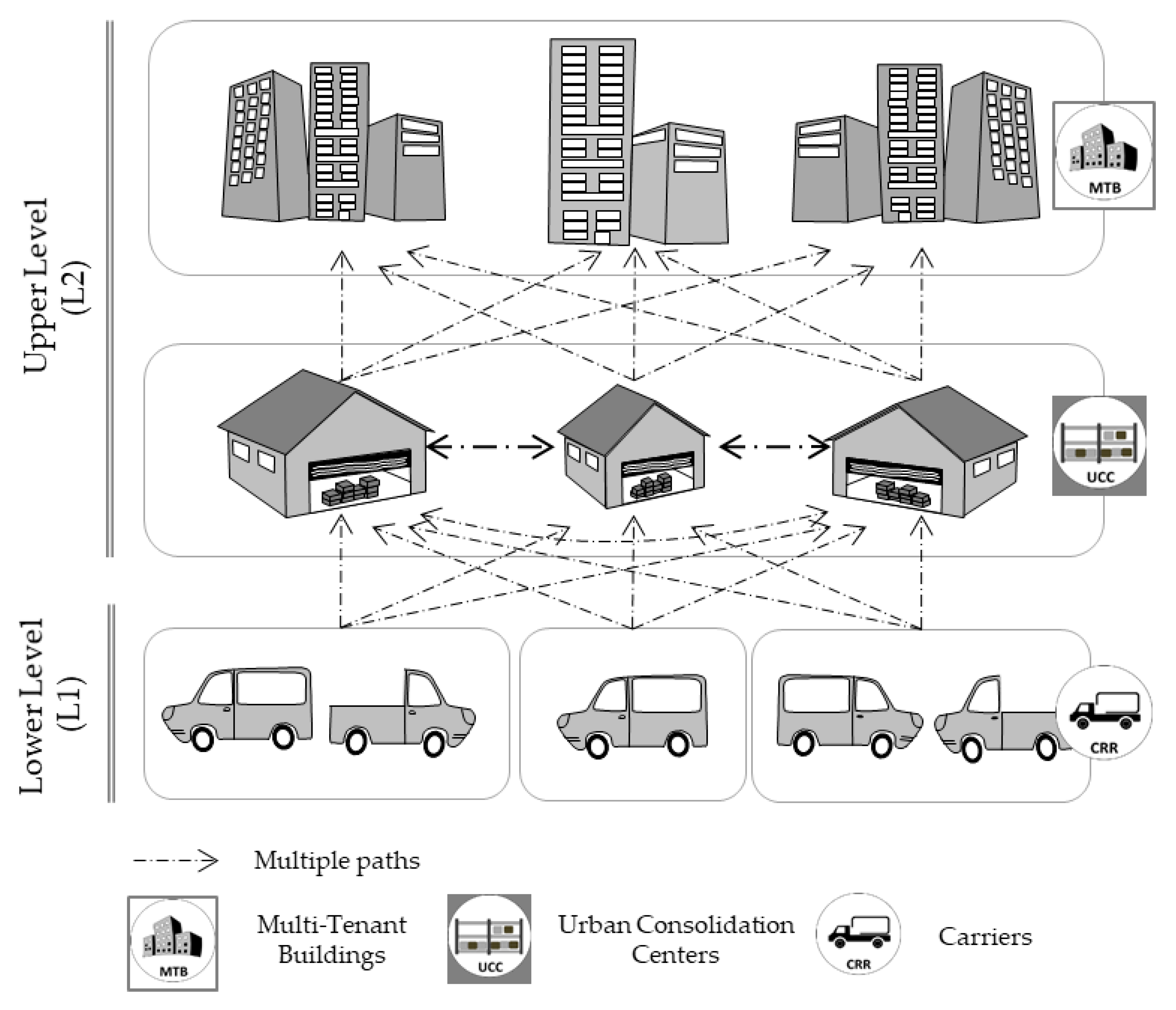
• The second distribution network is with an open transport infrastructure, where various transport operators share space, handling resources and other operational services. In this configuration, the UCCs are interconnected; therefore, the carriers can choose among alternative solutions from their depot to an MTB in order to optimize their own performance. These alternative solutions generate multiple potential paths for the parcels. For instance, many UCCs can be used in a chain to deliver parcels to the final destination. In this network, the transport operations performed by the transport companies are considered as fully integrated. Hence, this network is labeled as FI (Full Integration). Figure 2 represents this distribution network with integration of the urban consolidation centers.

The second key definition is about the pooling of parcels. From a general point of view, pooling consists in sharing of business processes and resources to provide scalable services for customers to gain optimized performance. Pooling requires companies to collaborate; for instance, by using joint resources with finite capacities. In the field of transport, sharing the urban consolidation centers among transport operators is a way to improve the overall performance of the distribution. Another way to further improve the transport performance could be the pooling of the vehicles.

Therefore, in the remainder of this study, we assume that the distribution network can be operated in different modes, whether the pooling of parcels from different carriers in the same truck is allowed or not. These modes are described as follows:

• In the first mode, labeled as NoPooling (NP), the carriers are independent and the parcels coming from different source nodes (i.e., carriers’ depot) cannot share the same truck.
• In the second mode, labeled as WithPooling (WP), parcels from different source nodes to the same destination can be pooled in the same truck. Notice that the pooling potentially applies to all the arcs of the network, but its impact on the parcels flows is different depending on the degree of connectivity of the network.

In order to evaluate the transport flows of these various distribution networks and to carry out some comparisons between them, we made the following assumptions:

• We focused on an overall (i.e., macroscopic) evaluation of the flows. Consequently, we focused on a mid-term evaluation without considering the routes optimization of the individual trucks.
• We focused on a one-day period of operation for the performance evaluation. Therefore, we did not address the specific time aspects (such as arrival time of the parcel) related to the entities (UCCs, MTBs) and to the flows between them.
• We carried out performance evaluations based on a cumulative assessment of the costs (i.e., distance, time, etc.) occurring on a full path from source to destination (which consists of many arcs shown in Figure 1 and Figure 2).
• We focused on the forward distribution flows from the carriers (i.e., sources) to the final destinations (i.e., MTB). The number of parcels returned from the MTB is usually very low; therefore, the return flows are not as critical as the forward flows. Consequently, no return flows from the MTBs back to the carrier are taken into account in this study.
• We assumed that the local administrative authorities can impose some limitations on the truck flows on certain arcs (i.e., maximum number of trucks). This limitation is in line with the aim of being able to reduce the negative impacts of freight transport in certain parts of the city. One example is the work of [35], which proposes an approach to reduce the environmental footprint of freight deliveries near sensitive urban facilities such as hospitals, schools, and retirement homes.
• Lastly, we assumed that the goal of UCCs located near the city center is to ban direct deliveries from a source to a final destination in order to reduce congestion or other environmental factors in densely populated areas. Therefore, in our model, the parcels flows have to cross UCCs in their journey from a carrier to an MTB, instead of being directly delivered to MTB.

3.2. Modeling of the Distribution Networks

The studied multi-commodity network flow (MCNF) problem is modeled by a directed graph $G=\left(V, A\right)$ where $V$is the set of nodes and $A$ the set of arcs. The nodes are associated to each entity of the distribution network: UCCs, MTBs, and the carriers’ depots. For each node $i\in V$, the set labeled suc(i) (respectively, pre(i)) characterizes the set of successors (respectively, predecessors) of node i in graph G.

Set $A$ of arcs of the graph is partitioned into two subsets A₁ and A₂, corresponding to the two levels (L1 and L2) of the distribution network (see Figure 1 and Figure 2). These two separate levels are defined as follows:

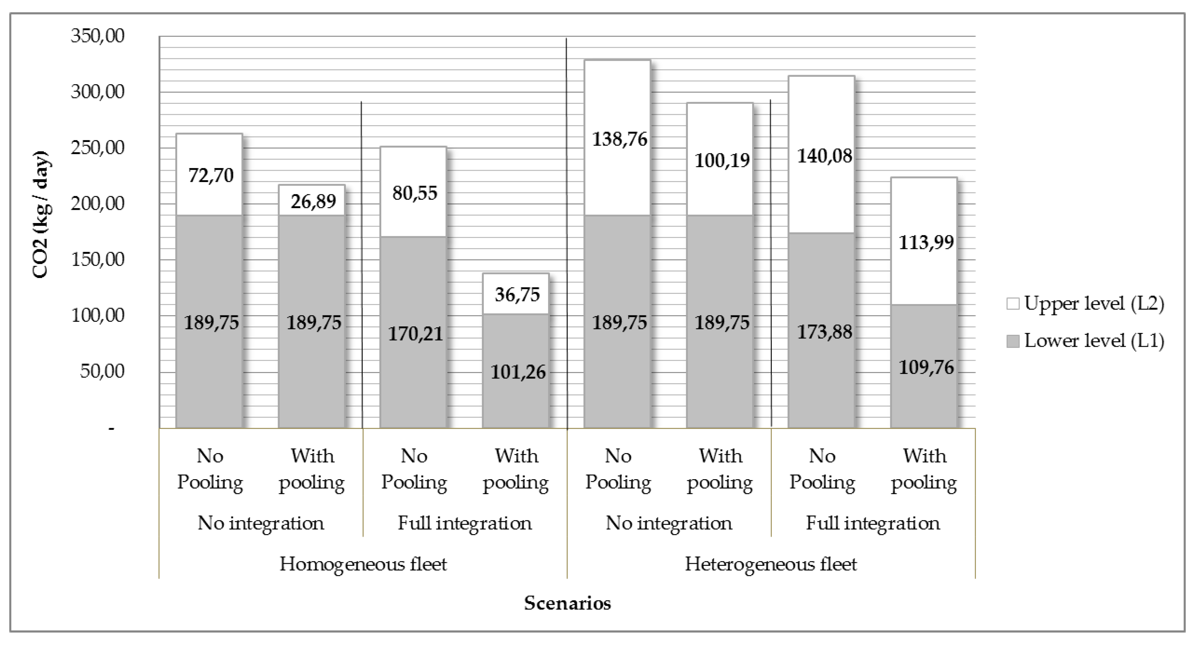
• The flows between carriers and UCCs (i.e., lower level) make up the first level of the two-tiers distribution problem. This level, labeled as L1, characterizes the part of the transportation network used by larger vehicles, which use traffic lanes outside the city center.
• The flows between UCCs and MTBs (i.e., upper level), make up the second level of the two-tiers distribution problem. This level is labeled as L2. The flows (parcels) exchanged between two UCCs are also considered as a part of this level.

Set L defines the set of levels (i.e., L = {1,2}) and, set $A_l$ contains the level l arcs. A non-negative capacity $ca{p}_{i,j}$ is assigned to each arc $\left(i,j\right)\in A$ and characterizes the maximum number of parcels going through this arc. The arc capacity is expressed as a multiple of the capacities$\mathrm{of}\mathrm{trucks} TruckCa{p}_l$ used in level l $\in L$. A travel cost ($cos{t}_{i,j})$ is also defined for each arc, representing the distance between nodes i and j. In addition, we introduce set K of the delivery demands. Each delivery demand $k \left(k\in K\right)$ has to be delivered from the depot of the carrier i (i.e., source node) to MTB j (i.e., destination node). This demand is modeled by assigning a positive quantity of parcels ($suppl{y}_{k,i})$ at the source node i and by assigning the corresponding negative value ($-suppl{y}_{k,j})$ at the destination node j.

Variables $nb{t}_{i,j,k}$ and $nbtU{T}_{i,j,k}$ correspond to, respectively, the number of full and partial (incomplete) trucks needed to satisfy the demand k on arc (i,j). Variable $nbpU{T}_{i,j,k}$ is the quantity of parcels corresponding to an incomplete truck (less than a full truckload) of the total demand k assigned to arc (i,j). Integer variable $x_{i,j,k}$ quantifies the number of parcels of demand k on arc (i,j).

We propose two formulations of the studied problems based on whether the pooling of parcels from different carriers in the same truck is allowed (Formulation WithPooling) or not (Formulation NoPooling). Both formulations use the same objective function (see Equation (1)) which minimizes the cumulated distances of all trucks over all the arcs of the graph. Equation (2) represents the capacity constraint on each arc (i,j). Equation (3) is the flow balance equation between input and output on arcs, which has to be verified for each node and for each demand. Equation (4) represents the truckload capacity constraint, which is used to calculate the number of full trucks and the number of parcels in the incomplete trucks. Equation (5) limits the number of parcels in an incomplete truck to the capacity of this truck. Equation (6) calculates the number of incomplete trucks, which is equal to zero or one. Equations (7)–(9) are corresponding equations in WithPooling formulation to Equations (4)–(6) of NoPooling formulation. Equation (6) and Equation (9) are linearized in the model implemented in the solver.

$$\left(\mathrm{NoPooling}\right)\min {\displaystyle \sum }_{\left(i,j\right)\in A, k\in K} cos{t}_{i,j}\ast \left(nb{t}_{i,j,k}+nbtU{T}_{i,j,k}\right)$$

(1)

s.t.

$${{\displaystyle \sum }}_{k \in K}{x}_{i,j,k}\le ca{p}_{i,j} \forall \left(i,j\right)\in A$$

(2)

$${{\displaystyle \sum }}_{j \in suc\left(i\right)}{x}_{i,j,k} - {{\displaystyle \sum }}_{j \in pre\left(i\right)}{x}_{i,j,k} =suppl{y}_{k,i }\forall i \in V, \forall k \in K$$

(3)

$$x_{i,j,k}= nb{t}_{i,j,k} · TruckCa{p}_l+nbpU{T}_{i,j,k} \forall l\in L, \forall \left(i,j\right)\in A_l,\forall k \in K$$

(4)

$$nbpU{T}_{i,j,k}\le TruckCa{p}_l-1 \forall l\in L, \forall \left(i,j\right)\in A_l, \forall k \in K$$

(5)

$$nbtU{T}_{i,j,k}=[nbpU{T}_{i,j,k} / TruckCa{p}_l] \forall l\in L, \forall \left(i,j\right)\in A_l, \forall k \in K$$

(6)

The formulation WithPooling is a variant of the previous model, where the variables$nb{t}_{i,j}$, $nbtU{T}_{i,j}$and $nbpU{T}_{i,j}$are no longer dependent on index k due to pooling of all demands.

$$\left(\mathrm{WithPooling}\right)\min {\displaystyle \sum }_{\left(i,j\right)\in A } cos{t}_{i,j}\ast \left(nb{t}_{i,j}+nbtU{T}_{i,j}\right)$$

s.t.    (2)–(3)

$${{\displaystyle \sum }}_{k \in K}{x}_{i,j,k}= nb{t}_{i,j} · TruckCa{p}_l+nbpU{T}_{i,j} \forall l\in L, \forall \left(i,j\right)\in A_l$$

(7)

$$nbpU{T}_{i,j}\le TruckCa{p}_l-1 \forall l\in L, \forall \left(i,j\right)\in A_l$$

(8)

$$nbtU{T}_{i,j}=[nbpU{T}_{i,j} / TruckCa{p}_l] \forall l\in L, \forall \left(i,j\right)\in A_l$$

(9)

3.3. Experimental Setup

In order to evaluate the distribution networks (Figure 1 and Figure 2), we created some test scenarios based on the freight distribution in Tokyo. It should be recalled that the capital of Japan is one of the largest metropolitan areas in the world (about 39 million inhabitants) and one of the largest economies in the world. We firstly introduce the context of the distribution of Tokyo city as to why it has been chosen to define our test scenarios. Then, we describe the input parameters common to all test scenarios followed by the input factors, which vary in each test scenario. Lastly, we describe the performance indicators used to evaluate the distribution networks.

3.3.1. Distribution Context of Tokyo

The approach proposed in this paper for modeling and performance evaluation is generic and has no strong limitation regarding the number of MTBs and UCCs. However, our test scenarios are based on the logistics practices currently implemented in some parts of Tokyo, which is comparable to the situation depicted in Figure 1 (i.e., No Integration). It can be described as follows:

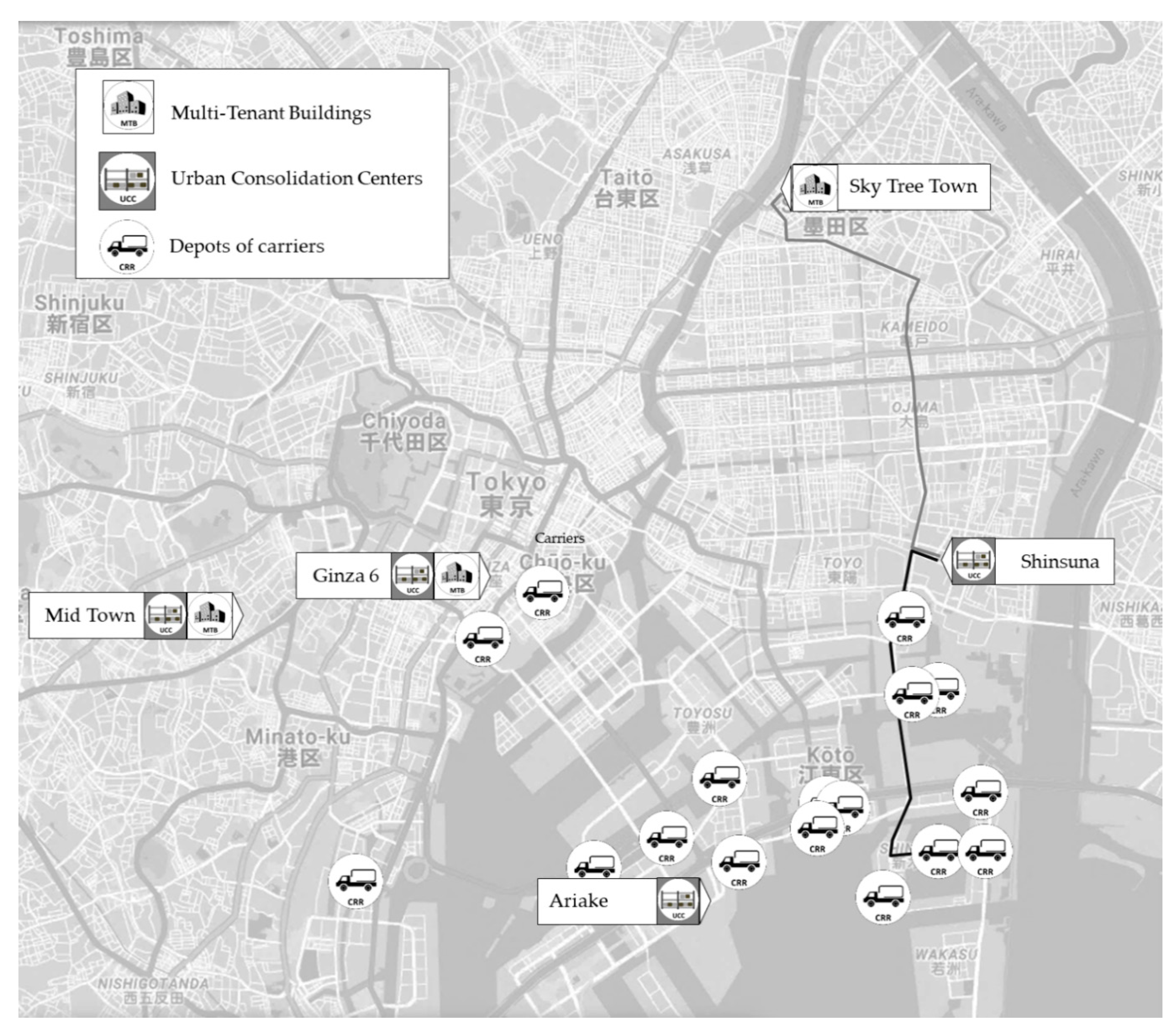
• There are three main MTBs of Tokyo: Ginza six (G6) in the Chuo ward, Tokyo Sky Tree Town (TT) in the Sumida ward and Tokyo Midtown (MT) in the Minato ward as shown in Figure 3.
• Four UCCs are in charge to distribute the parcels to these MTBs. The UCCs of Midtown and Ginza six are located in the basement of the MTB itself and serve to perform consolidation of deliveries addressed to the different floors. The MTB “Tokyo Sky Tree Town” is supplied by two external UCCs (Ariake and Shinsuna) as shown in Figure 2. All of these UCCs are dedicated to a specific MTB and there is no integration between them.
• We have also considered many depots, owned by the carriers, mainly located in the area of the Tokyo bay where the goods are arriving by linehaul trucks. Each carrier can serve any of the MTBs.

Figure 3 gives the locations of MTBs, UCCs, and carriers on the city map. It also shows a possible path from a carrier to Shinsuna UCC and from this UCC to Tokyo Sky Tree Town as an example.

3.3.2. Common Input Parameters

There are two main input parameters, which are fixed for all scenarios:

• The demands ($suppl{y}_{k,i})$, which are based on a combination of real and estimated delivery data. The real data comes from a major transportation company and logistics provider, operating the UCC at the Ginza six in Tokyo. The demands of the other MTBs are estimated using a proportional rule according to the surface area ratio of the considered MTB and Ginza six. Based on the real data, 18 carriers have been used in the distribution of parcels to the MTB terminals; one of these carriers has a dominant position and covers 43% of deliveries, whereas the top four carriers cover 88% of the demand.
• The cost ($cos{t}_{i,j})$ is the distance from node i to node j. The distances are average of the three distances obtained from Google Maps at 07:00 a.m., 11:00 a.m., and 2:00 p.m. in order to integrate the different traffic congestion situations. UCCs in Ginza six and Mid Town are located within these buildings; therefore, in these two cases, the distances $(cos{t}_{i,j}$) between UCC and MTB equals to zero.

3.3.3. Tests Scenarios

The tests scenarios are created using different input factors, which are as follows:

• Two possible values (45 or 180 parcels) for the capacity of the trucks (TruckCapl) have been considered. The lower capacity (i.e., 45 parcels) corresponds to a scenario where small trucks are used in the last-mile delivery starting from the UCC. These could be Light Electric Freight Vehicles as they are quiet, agile, emission-free, and take less space than conventional trucks and vans. The higher capacity (i.e., 180 parcels) corresponds to the average number of parcels for a three-ton truck, which is commonly used by the carriers. Consequently, we created two sets of possible scenarios based on types of vehicle in the network: either a homogenous fleet (HM), in which all vehicles have the same capacity over the entire network (180-180), or a heterogeneous fleet (HT) (45-180), with lower-capacity vehicles in the upper level (i.e., for $\left(i,j\right)\in A_2$) and larger vehicles in the lower level of the network (i.e., for $\left(i,j\right)\in A_1$).

Table 1. List of scenarios.

No.	Scenario Abbreviation	Integration	Pooling	Arcs Capacities	Trucks Capacities in A1 and A2
1	NP-NI-LI-HM	No	No	Limited	180-180
2	WP-NI-LI-HM	No	Yes	Limited	180-180
3	NP-FI-LI-HM	Yes	No	Limited	180-180
4	WP-FI-LI-HM	Yes	Yes	Limited	180-180
5	NP-NI-LI-HT	No	No	Limited	45-180
6	WP-NI-LI-HT	No	Yes	Limited	45-180
7	NP-FI-LI-HT	Yes	No	Limited	45-180
8	WP-FI-LI-HT	Yes	Yes	Limited	45-180
9	NP-NI-UL-HM	No	No	Unlimited	180-180
10	WP-NI-UL-HM	No	Yes	Unlimited	180-180
11	NP-FI-UL-HM	Yes	No	Unlimited	180-180
12	WP-FI-UL-HM	Yes	Yes	Unlimited	180-180
13	NP-NI-UL-HT	No	No	Unlimited	45-180
14	WP-NI-UL-HT	No	Yes	Unlimited	45-180
15	NP-FI-UL-HT	Yes	No	Unlimited	45-180
16	WP-FI-UL-HT	Yes	Yes	Unlimited	45-180

shows the full list of test scenarios resulting from these input factors.

• The degree of integration between the UCCs, which includes two levels: NI (No Integration) or FI (Full Integration).
• Whether the pooling of parcels is allowed or not: WP (With Pooling) or NP (No Pooling).
• The arcs capacities $ca{p}_{i,j}$of the network are unlimited (UL) or limited (LI). In the latter case, the values are assigned to the arcs in order to limit the emissions on a sub-area of the network.

3.3.4. Performance Indicators

In addition to the cumulated total distance of the trucks (TD) provided by the objective function (Equation (1)), some other performance indicators, including some sustainable development indicators (i.e., emissions) have also been calculated in a post-optimization stage. The list of indicators is defined below:

• The cumulated total distance of the trucks TD (i.e., Equation (1)).
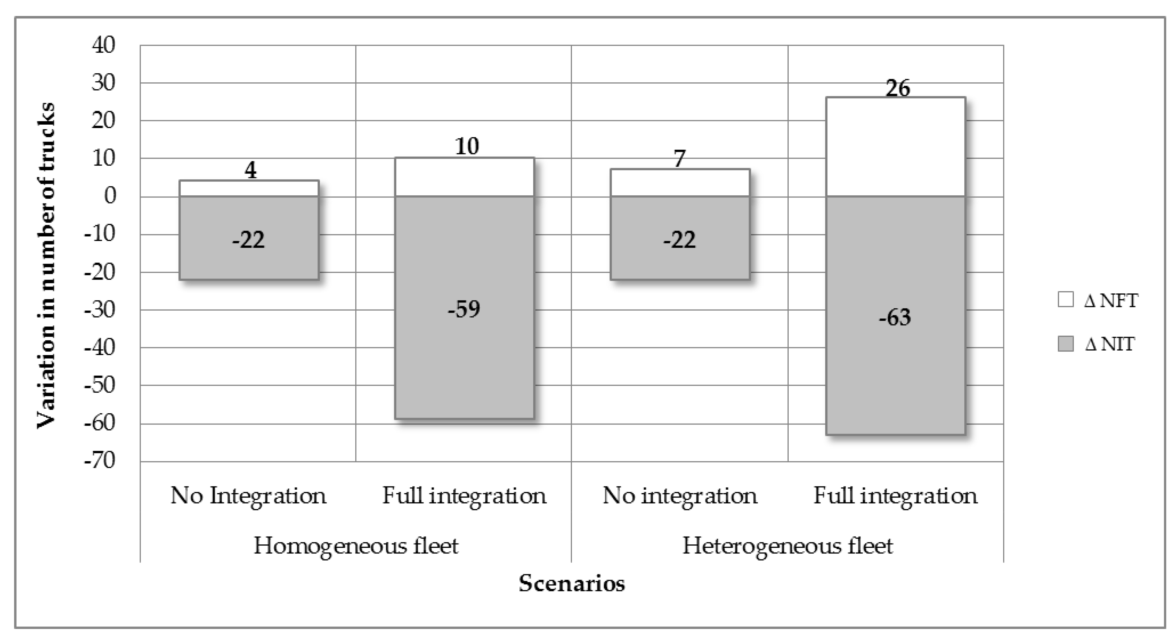
• The number of full trucks (NFT), the number of incomplete trucks (NIT), and the total number of trucks (NT) are calculated according to Equations (10)–(12) in the NoPooling formulation of the problem.

$$NFT={\displaystyle \sum }_{\left(i,j\right)in A, k\in K}nb{t}_{i,j,k}$$

(10)

$$NIT={\displaystyle \sum }_{\left(i,j\right)in A, k\in K}nbtU{T}_{i,j,k}$$

(11)

NT= NFT + NIT

(12)

Similar indicators are also calculated for the WithPooling formulation as well.

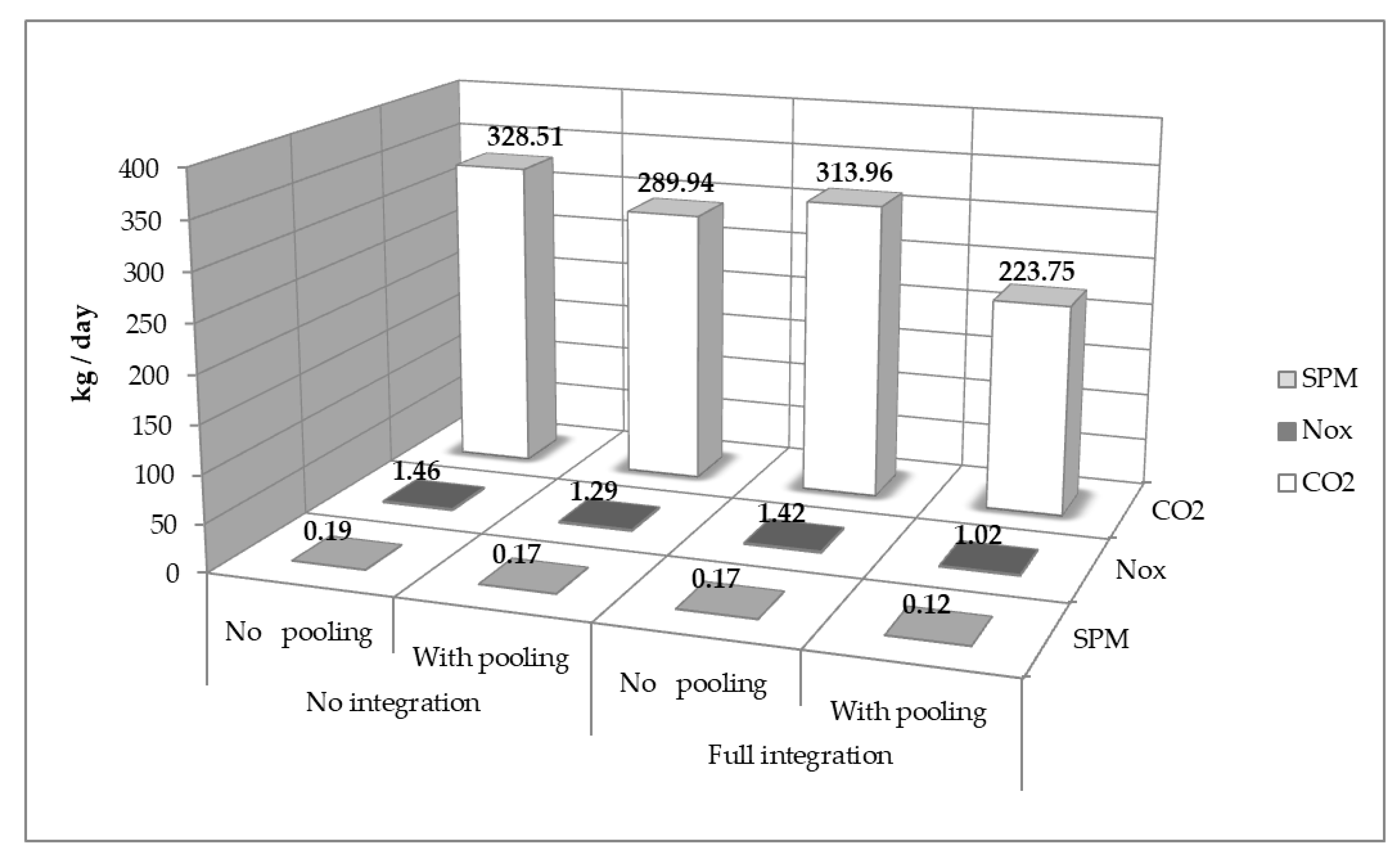
• The gas emissions (CO2, NOx) and the suspended particulate matter emissions (SPM) as defined in [36].
• In addition, we define the percent gap of a given indicator “X”, labeled as gapX (z1, z2). It is the relative variation of “X”, generated by switching the two-levels input factor z, and it is defined as: gapX (z1, z2) = (Xz1-Xz2)/Xz2, keeping all other input factors unchanged. For example, the percent gap in distance generated by the capacities of the network is reported as gapTD (LI, UL) = (TD_LI- TD_UL)/ TD_UL.

4. Results

The experiments (or scenarios) that have been conducted, aimed to assess the impact of the input factors on the performance indicators mentioned in the previous section. The models have been implemented with the IBM ILOG CPLEX solver.

Table 2. Characterization of the models.

Integration	Pooling	Demands	Nodes	Arcs	Constraints	Variables
NI	NP	72	25	76	32,124	24,193
NI	WP	72	25	76	8268	6301
FI	NP	72	25	96	36,456	27,649
FI	WP	72	25	96	9192	7,201

shows some information about the size of the models: number of nodes and arcs and also number of variables and constraints. The computation times to get the optimal solutions are less than 30 minutes in every experiment.

4.1. Total Cumulative Distance

Firstly, we focus on a network where the capacities on the arcs are limited (i.e., scenarios numbered 1-8). The results presented in Figure 4 and Figure 5 are intended to compare the total cumulated distance of the two distribution networks (NI and FI) depending on whether the capacities of trucks are homogeneous (HM) (180-180 parcels) or not (HT) (45-180 parcels) and depending also on whether the pooling of the parcels is allowed (WP) or not (NP). Figure 4 and Figure 5 show that the distance is significantly reduced when integration between UCCs is considered.

Table 3. Gap (percent) of total cumulated distance—Limited arcs capacities.

(a) Impact of Integration		(b) Impact of Pooling
Scenarios	gapTD (NI,FI)	Scenarios	gapTD (NP,WP)
NP-xx-LI-HM	11.7	xx-NI-LI-HM	18.4
WP-xx-LI-HM	38.9	xx-FI-LI-HM	43.5
NP-xx-LI-HT	9.9	xx-NI-LI-HT	11.9
WP-xx-LI-HT	22.3	xx-FI-LI-HT	23.9

and

Table 4. Gap (percent) of total cumulated distance—Full integration.

(a) Homogeneous Fleet		(b) Heterogeneous Fleet
Scenarios	gapTD (LI,UL)	Scenarios	gapTD (LI,UL)
NP-NII-xx-HM	0	NP-NI-xx-HT	0
WP-NI-xx-HM	0	WP-NI-xx-HT	0
NP-FI-xx-HM	28.4	NP-FI-xx-HT	7.7
WP-FI-xx-HM	4.6	WP-FI-xx-HT	15.6

give the impact (i.e., reduction gaps) of various input parameters. The "scenarios" column of these tables omits the comparison variable and replaces it with “xx”; for example, the label "NP-xx-LI-180" means that the impact of integration has been compared by reporting gapTD (NI, FI).

Table 3a shows that the gap varies between 10% and 39% when integration is considered. On the other hand, the distance reduction gap in Table 3b varies between 12% and 44% when the effect of pooling (WP or NP) is evaluated; proving a high impact of pooling on the distance reduction as compared to the integration. Furthermore, Table 3 shows that the reduction in distance is greater when the homogeneous fleet is used as compared to the case when heterogeneous fleet is used; for instance, this reduction drops from 43.5% to 23.9% in the case FI. Indeed, the limitation of the truck capacities at the upper level of the network (45 parcels) generates an increase in the number of trucks and therefore in distance.

Secondly, we analyze the impact of the arcs capacities by comparing the limited capacities scenarios (number 1 to 8) with unlimited capacities scenarios (number 9 to 16). The impact of arcs capacities on the total distance is provided by the gap indicator gap (LI, UL) in Table 4a,b. This indicator, which is characteristic of the dataset used, can be interpreted as a deviation from a minimum distance boundary that can only be reached if there is no capacity constraint on the arcs (i.e., gap = 0 means that the smallest minimum distance is reached).

These distance gaps in Table 4a,b are only for the full integration scenarios as the capacities of the arcs play no role (i.e., gap = 0) when there is no integration (NI), whether they are pooling or not. However, the impact of the arcs capacities of the network is significant with the integrated distribution network (FI) as seen in Table 4.

4.2. Emissions

Figure 6 and Figure 7 focus on emissions. The emission curves of the four possible combinations of the two input factors are plotted in these figures ("Pooling": WP or NP; "Integration": FI or NI). Figure 6 considers homogeneous fleet while Figure 7 is for heterogeneous fleet. Both of these figures have the same trend. The integrated version of the network allows a reduction of CO2 compared to the nonintegrated version; this reduction varies from 5% to 23% in the heterogeneous fleet case and varies from 5% to 36% in the homogeneous fleet case.

The reductions in all emissions (CO₂, NOx, SPM) are better for the FI-WP scenario, which exceeds the other three scenarios. Hence, the combination of pooling (WP) and network integration (FI) gives the best results in terms of emissions. This corresponds to a significant reduction in the cumulative total distance observed in the previous analysis (i.e., the TD indicator). The NI-WP scenario is intermediate in terms of emissions, demonstrating a very positive impact of pooling, even in non-integration (NI) scenarios. In contrast, FI-NP and NI-NP scenarios without pooling provide almost identical results that are the worst in terms of emission reductions.

Figure 8 focuses on the distribution of CO₂ emissions over the two levels of the distribution network (i.e., L₁ and L₂) in the different scenarios. This figure shows that the introduction of zero-emission vehicles such as Light Electric Freight Vehicles in the last few kilometers of delivery would significantly reduce CO₂ emissions by keeping only low-level emissions (grey bars). A comparison of FI-WP scenarios with homogeneous and heterogeneous fleets shows that the increase in emissions generated by the use of smaller trucks at the high level (FI-WP-LI-HT) can be offset by the use of zero-emission vehicles, reducing CO₂ emissions to get the same orders of magnitude (101 and 109 kg/day) for both scenarios FI-WP-LI-HM and FI-WP-LI-HT. The average reduction of the CO2 emissions for all scenarios is 35%.

4.3. Number of Trucks

In this last part, we evaluate the impact of the pooling on the number of trucks used in the whole network. We focus on the variation of the number of full trucks (Δ NFT) and the variation of the number of incomplete trucks (Δ NIT), depending on whether pooling is allowed or not. Figure 9 shows that in the four scenarios shown, pooling makes it possible, on the one hand, to increase very significantly the number of full trucks (white part of bars) and simultaneously reduces the number of incomplete trucks (grey bars). The most significant variations come from the scenarios with full network integration (FI) compared to the scenarios without integration (NI). For example, in the full network integration scenarios, heterogeneous fleet scenario reduces the number of incomplete trucks by 63 units (NIT decreased from 84 to 21) and increases the number of full trucks by 26 units (NFT increased from 21 to 46). The net reduction of the total number of trucks is significant for all scenarios, as shown in

Table 5. Impact of pooling: variation on the number of trucks in the two levels of the network.

Scenario	Total	Lower Level (L1)	Upper Level (L2)
xx-NI-LI-HM	−18 (−18%)	0	−18 (−64%)
xx-FI-LI-HM	−49 (−45%)	−29 (−40%)	−20 (−57%)
xx-NI_LI-HT	−15 (−12%)	0	−15 (−29%)
xx-FI-LI-HT	−37 (−28%)	−28 (−38%)	−9 (−16%)

("Total" column). The average reduction in the number of trucks for all scenarios is 29%. We can conclude that pooling has a very strong impact on reducing the number of trucks. The breakdown of this variation by network level shows that scenarios without integration (NI) are unable to reduce the number of trucks, which is in line with the fact that these scenarios are very constrained in terms of flow because they do not offer transport alternatives from the depot to the UCC. Table 5 also shows that scenarios with integration (FI) generate a higher average reduction on the lower level. This reduction is less important when heterogeneous fleet is used because the increased number of lower capacity trucks in the upper level balances the decreasing effect of pooling.

5. Conclusions

In this article, we propose a methodology for evaluating the performance of a parcels distribution network in urban logistics. The originality of this methodology is as follows:

• The representation of the distribution problem in the form of a multi-commodity network flow which is, to our knowledge, a novelty in the field of urban logistics. The linear programming model makes it possible to optimize the total distance traveled and makes it possible to evaluate the impact in terms of emissions of the studied network. This model encompasses the UCCs, which are central elements in vertical collaboration; it also offers the possibility to limit the impact of the distribution flows in specific areas by using the arc capacities of the network.
• We reported several comparisons. Firstly, the comparison of two types of distribution networks with different degrees of connectivity (i.e., integrated (FI) vs. nonintegrated (NI) networks); these two types of networks correspond to the current state (NI) and a proposed future state of the distribution system (FI). Secondly, we reported the comparison of two types of organization regarding the parcel distribution (With Pooling (WP) or No Pooling (NP)).
• Lastly, this approach is generic and can be applied to optimize parcel distribution in city centers of large urban areas.

The experimental study of the distribution of parcels to the MTBs (large shopping centers) in the city of Tokyo highlights the benefits of using a fully integrated distribution network compared to a network without integration. A very important reduction of the traveled distance (up to 39%) and a significant reduction in emissions (up to 36% of CO2 emissions) can be obtained in fully integrated distribution networks. It also highlights the impact of pooling, which brings a reduction of up to 29% of the distance traveled compared to no pooling organization. Our study also makes it possible to quantify the reduction in emissions due to the introduction of zero-emission vehicles, such as Light Electric Freight Vehicles at the upper level (L2) of the network; this reduction is about 35% on average in all scenarios. Overall, the combination of an integrated network and the pooling of parcels improves the reduction of emissions, travel distances, and number of trucks, leading to the implementation of sustainable urban freight transport systems.

Future studies will focus on the following issues: (i) introducing time in the flow modeling, which is a key component for enhancing the model in order to carry out multiperiod optimization on a given planning horizon and also to be able to represent the behavior of the UCC over time (i.e., load over time); (ii) carrying out financial assessments of the different networks, taking into account the administrative costs of the UCCs; (iii) study the impact of new multi-tenant buildings resulting from the implementation of transportation infrastructure dedicated to the development of a new generation of ultra-high-speed trains in Tokyo; (iv) applying our distribution modeling approach to other cities in order to carry out comparative studies between the practices used in different countries in order to identify best practices.

References

1. Taniguchi, E.; Thompson, R.G.; Yamada, T. New opportunities and challenges for city logistics. Transp. Res. Procedia 2016, 12, 5–13. [Google Scholar] [CrossRef] [Green Version]
2. Anand, N.; van Duin, R.; Quak, H.; Tavasszy, L. Relevance of City Logistics Modelling Efforts: A Review. Transp. Rev. 2015, 35, 701–719. [Google Scholar] [CrossRef]
3. Roca-Riu, M.; Estrada, M. An evaluation of urban consolidation centers through logistics systems analysis in circumstances where companies have equal market shares. Soc. Behav. Sci. 2012, 39, 786–806. [Google Scholar] [CrossRef] [Green Version]
4. Edwards, T.J.; Kumphai, W. Sustainability in Multi-tenant Office Buildings: Anatomy of a LEED EBOM Program. Energy Eng. 2012, 109, 7–23. [Google Scholar] [CrossRef]
5. McDermott, D.R. An Alternative Framework for Urban Goods Distribution: Consolidation. Transp. J. 1975, 15, 29–39. [Google Scholar]
6. Holguín-Veras, J.; Patil, G.R. A Multicommodity Integrated Freight Origin–destination Synthesis Model. Netw. Spat. Econ. 2008, 8, 309–326. [Google Scholar] [CrossRef]
7. Crainic, T.G. Service network design in freight transportation. Eur. J. Oper. Res. 2000, 122, 272–288. [Google Scholar] [CrossRef]
8. Yang, J.; Guo, J.; Ma, S. Low-carbon city logistics distribution network design with resource deployment. J. Clean. Prod. 2016, 119, 223–228. [Google Scholar] [CrossRef]
9. Yang, L.; Cai, Y.; Hong, J.; Shi, Y.; Zhang, Z. Urban Distribution Mode Selection under Low Carbon Economy—A Case Study of Guangzhou City. Sustainability 2016, 8, 673. [Google Scholar] [CrossRef] [Green Version]
10. Li, S.; Wei, Z.; Huang, A. Location Selection of Urban Distribution Center with a Mathematical Modeling Approach Based on the Total Cost. IEEE Access 2018, 6, 61833–61842. [Google Scholar] [CrossRef]
11. Crainic, T.G.; Ricciardi, N.; Storchi, G. Models for Evaluating and Planning City Logistics Systems. Transp. Sci. 2009. [Google Scholar] [CrossRef] [Green Version]
12. Taniguchi, E.; Heijden, R.E.C.M.V.D. An evaluation methodology for city logistics. Transp. Rev. 2000, 20, 65–90. [Google Scholar] [CrossRef]
13. Hezarkhani, B.; Slikker, M.; Van Woensel, T. Gain-sharing in urban consolidation centers. Eur. J. Oper. Res. 2019, 279, 380–392. [Google Scholar] [CrossRef]
14. Firdausiyah, N.; Taniguchi, E.; Qureshi, A.G. Modeling city logistics using adaptive dynamic programming based multi-agent simulation. Transp. Res. Part E Logist. Transp. Rev. 2019, 125, 74–96. [Google Scholar] [CrossRef]
15. Rabe, M.; Klueter, A.; Wuttke, A. Evaluating the consolidation of distribution flows using a discrete event supply chain simulation tool: Application to a case study in Greece. In Proceedings of the 2018 Winter Simulation Conference (WSC), Gothenburg, Sweden, 9–12 December 2018; pp. 2815–2826. [Google Scholar] [CrossRef]
16. Cleophas, C.; Cottrill, C.; Ehmke, J.F.; Tierney, K. Collaborative urban transportation: Recent advances in theory and practice. Eur. J. Oper. Res. 2019, 273, 801–816. [Google Scholar] [CrossRef]
17. Allen, J.; Browne, M.; Woodburn, A.; Leonardi, J. The Role of Urban Consolidation Centres in Sustainable Freight Transport. Transp. Rev. 2012, 32, 473–490. [Google Scholar] [CrossRef]
18. Allen, J.; Browne, M.; Woodburn, A.G.; Leonardi, J. A review of urban consolidation centres in the supply chain based on a case study approach. Supply Chain Forum Int. J. 2014, 15, 100–112. [Google Scholar] [CrossRef] [Green Version]
19. Browne, M.; Woodburn, A.; Allen, J. Evaluating the potential for urban consolidation centres. Eur. Transp. 2007, 35, 46–63. [Google Scholar]
20. Van Duin, J.H.R.; van Kolck, A.; Anand, N.; Tavasszy, L.A.; Taniguchi, E. Towards an Agent-Based Modelling Approach for the Evaluation of Dynamic Usage of Urban Distribution Centres. Procedia—Soc. Behav. Sci. 2012, 39, 333–348. [Google Scholar] [CrossRef] [Green Version]
21. Cherrett, T.; Allen, J.; McLeod, F.; Maynard, S.; Hickford, A.; Browne, M. Understanding urban freight activity—Key issues for freight planning. J. Transp. Geogr. 2012, 24, 22–32. [Google Scholar] [CrossRef] [Green Version]
22. Battaia, G.; Faure, L.; Marqués, G.; Guillaume, R.; Montoya-Torres, J.R. A Methodology to Anticipate the Activity Level of Collaborative Networks: The Case of Urban Consolidation. Supply Chain Forum 2014, 15, 70–82. [Google Scholar] [CrossRef] [Green Version]
23. Simoni, M.D.; Bujanovic, P.; Boyles, S.D.; Kutanoglu, E. Urban consolidation solutions for parcel delivery considering location, fleet and route choice. Case Stud. Transp. Policy 2018, 6, 112–124. [Google Scholar] [CrossRef]
24. Panero, M.; Hyeonshic, S.; Lopez, D. Urban Distribution Centers: A Means to Reducing Freight Vehicle Miles Traveled; Final Report; New York University: New York, NY, USA, 2011. [Google Scholar]
25. Browne, M.; Allen, J.; Leonardi, J. Evaluating the use of an urban consolidation centre and electric vehicles in central London. IATSS Res. 2011, 35, 1–6. [Google Scholar] [CrossRef] [Green Version]
26. Van Rooijen, T.; Quak, H. Local impacts of a new urban consolidation centre—The case of Binnenstadservice.nl. Procedia—Soc. Behav. Sci. 2010, 2, 5967–5979. [Google Scholar] [CrossRef] [Green Version]
27. Holguín-Veras, J.; Amaya Leal, J.; Sanchez-Diaz, I.; Browne, M.; Wojtowicz, J. State of the art and practice of urban freight management Part II: Financial approaches, logistics, and demand management. Transp. Res. Part Policy Pract. 2018. [Google Scholar] [CrossRef]
28. Björklund, M.; Johansson, H. Urban consolidation centre—A literature review, categorisation, and a future research agenda. Int. J. Phys. Distrib. Logist. Manag. 2018, 48, 745–764. [Google Scholar] [CrossRef] [Green Version]
29. Ahuja, R.K.; Magnanti, T.L.; Orlin, J.B. Network Flows: Theory, Algorithms, and Applications, 1st ed.; Pearson: Englewood Cliffs, NJ, USA, 1993. [Google Scholar]
30. Karp, R.M. On the Computational Complexity of Combinatorial Problems. Networks 1975, 5, 45–68. [Google Scholar] [CrossRef]
31. Assad, A.A. Multicommodity network flows—A survey. Networks 1978, 8, 37–91. [Google Scholar] [CrossRef]
32. Barnhart, C.; Hane, C.A.; Vance, P.H. Using Branch-and-Price-and-Cut to Solve Origin-Destination Integer Multicommodity Flow Problems. Oper. Res. 2000, 48, 318–326. [Google Scholar] [CrossRef]
33. Farvolden, J.M.; Powell, W.B.; Lustig, I.J. A Primal Partitioning Solution for the Arc-Chain Formulation of a Multicommodity Network Flow Problem. Oper. Res. 1993, 41, 669–693. [Google Scholar] [CrossRef]
34. Barnhart, C.; Sheffi, Y. A Network-Based Primal-Dual Heuristic for the Solution of Multicommodity Network Flow Problems. Transp. Sci. 1993, 27, 102–117. [Google Scholar] [CrossRef]
35. Qureshi, A.G.; Taniguchi, E.; Iwase, G. A Vehicle Routing Model Considering the Environment and Safety in the Vicinity of Sensitive Urban Facilities. In City Logistics 1; John Wiley & Sons, Ltd.: Hoboken, NJ, USA, 2018; Chapter 18; pp. 343–357. [Google Scholar] [CrossRef]
36. NILIM, National Institute of Land and Infrastructure Management. Quantitative Appraisal Index Calculations Used for Basic Unit Computation of CO2, NOx, SPM; National Institute of Land and Infrastructure Management: Tsukuba, Japan, 2003. (In Japanese) [Google Scholar]
Figure 1. Transportation network with no integration (NI).
Sustainability 12 02180 g001
Figure 2. Transportation network with full integration (FI).
Sustainability 12 02180 g002
Figure 3. A Tokyo map extract with multi-tenant buildings (MTBs), urban consolidation centers (UCCs), and depots of carriers.
Sustainability 12 02180 g003
Figure 4. Total cumulated distances (TD)—Homogeneous fleet (HM).
Sustainability 12 02180 g004
Figure 5. Total cumulated distances (TD)—Heterogeneous fleet (HT).
Sustainability 12 02180 g005
Figure 6. Emissions: CO2, NOx, suspended particulate matter (SPM)—Homogeneous fleet (HM).
Sustainability 12 02180 g006
Figure 7. Emissions: CO2, NOx, SPM—Heterogeneous fleet (HT).
Sustainability 12 02180 g007
Figure 8. Emissions (CO2) in the different network levels.
Sustainability 12 02180 g008
Figure 9. Impact of pooling on the variation of number of trucks.
Sustainability 12 02180 g009