Abstract
A major consideration for consumers and the residential construction industry is the cost–benefit and break-even of various sustainable construction options. This research provides a publicly available simulation that allows users to compare baseline construction options versus sustainable options and evaluates both break-even costs as well as environmental effects. This R Shiny Monte Carlo simulation uses common pseudo-random number streams for replicability and includes options for solar, rainwater harvesting, wells, Icynene foam, engineered lumber, Energy Star windows and doors, low flow fixtures, aerobic/non-aerobic/city waste treatment, electric versus gasoline vehicles, and many other options. This is the first simulation to quantify multiple sustainable construction options, associated break-even points, and environmental considerations for public use. Using user default parameters, coupled with a 100% solar solution for a baseline 3000 square foot/279 square meter house with 2 occupants results in a break-even of 9 years. Results show that many of the sustainable options are both green for the environment and green for the pocketbook.
1. Introduction
Reducing the impact of the built environment is a necessary step to address concerns of climate change, as well as population growth. Green building codes and certifications (GBCCs) have arisen to help provide best practice for green construction. Understanding which codes actually result in effective environmental changes that are positive for the consumer is necessary [1]. Incorporating requirements into GBCC systems improves environmental performance 15–25% across 12 environmental impact categories when compared with the construction of a standard office building, as defined by the National Institute of Standards and Technology [1].
In a recent study, electricity, tap water consumption, and employee commuting dominated 10 out of 12 environmental impact categories, categories that included global warming; human health consequences; eutrophication, acidification, and use of water; and smog formation. For land use impacts, wood products contributed the most (perhaps, unsurprisingly) [2]. Overall, GBCCs have been found to cause up to 25% fewer environmental impacts than standard building techniques. Specific improvements include acidification (25%), human health—respiratory (24%), and global warming (22%) [2].
Net Zero (or even Net Positive) construction involves the design of facilities that either consume no net energy (demand less supply) or that produce more energy than consumed [3], reducing global warming. Net Zero construction may even power user transportation [4]. Rainwater harvesting removes the stress on below-ground and groundwater sources for both residential and business construction (including hospitals) [5,6].
Evaluating cost–benefit for certain elements of sustainable construction is not unique, and the evidence is both international and mixed. A study in Israel demonstrated lower electricity and water bills for certain sustainable interventions in schools, but there was no achievable or meaningful break-even [7]. A United States study illustrated that the construction costs were larger up front for green-certified residences, and that these houses demanded a significant price premium [8]. Sun, Chen, Wang, Lo, Yau, and Wu [9] demonstrated increased costs for green construction between 1.58% and 9.3% in Taiwan. Dwaikat and Ali conducted an empirical review of evidence associated with green building. They discovered a cost premium range for green construction between −0.4% and 21% in 17 studies [10]. These findings may be due partially to different definitions of “green” construction (i.e., different elements) and geography. Up-front costs exist.
Still, the break-even for such costs may be trivial, depending on the consumer’s needs or desires. A study in China showed green building can generate incremental economic benefits [11]. Liu and Liu provided a decision framework for sustainable construction options partially based upon mortgage analysis. In their framework, they focused on thermal efficiency in Australia and found that a 45% improvement in energy consumption would be amortized in 25 years [12]. This type of break-even analysis is important for both the consumer and the builder. In New Zealand, a study indicated that the New Zealand Green Building Commission’s Homestar standards may deliver operational savings, but that many residences are unable to experience the savings estimates suggested [13].
Qualitative and policy analysis of cost–benefits also exist in the literature. A qualitative essay provided empirical evidence of cost offsets and break-even points for some but not all sustainable construction techniques employed [14]. With increased legislation requiring sustainable construction, such as California’s measure to require 100% solar offset of new residential construction [15], affordability is likely to be affected [16]. When considering both criteria (sustainability and affordability), policymakers and consumers need to understand both the short-term and the long-term effects.
These studies provide the basis for building a flexible simulation, one which evaluates both costs and environmental impact. The simulation itself was motivated by a research residence. The research home, once the highest certified home for sustainable construction based on the National Association of Homebuilders standards [4], exists on 100% solar and 100% rainwater harvesting. The user interactive simulation is based on cost, demand, supply, and environmental considerations. The primary hypothesis is that some elements of green construction might also be green for the pocketbook as well. Using distributions based upon known costs and relationships, we propose a simulation that allows users to investigate singularly or simultaneously various green construction options. Break-even analysis is therefore produced.
2. Materials and Methods
In this Monte Carlo simulation study, we evaluate break-even considerations, environmental impacts, and efficacy of multiple sustainable building innovations for residences. Included in the simulation are user options for lumber selection, insulation selection, window and door selection, the water system, the electrical system, the water heating system, geothermal heating and cooling, and vehicle selection. Vehicle selection is an important consideration, as an electric vehicle (EV) powered 100% by the home requires additional solar power but may reduce emissions and eliminates the owner’s need for gasoline, all of which have impacts on costs and the environment.
A simulation of costs over time, based on construction materials selection, provides information about the cost and environmental effects of residential construction decisions. Measured outputs include cost, demand for water and electricity, CO2e emissions, trees required for the construction process, and water required to support the demand of occupants. The simulation is implemented in R Shiny [17] and freely available here: https://rminator.shinyapps.io/sustain4/. Figure 1 is the motivation for this simulation, a sustainable residence [18].
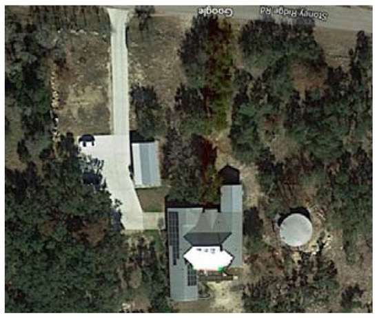
Figure 1.
The residence as constructed.
2.1. Acquisition Costs and Selection of Lumber, Engineered vs. Traditional
Finger-jointed studs use reclaimed wood that might otherwise be discarded (Figure 2). They are straighter and result in less wood wasted. Further, they have a strong vertical load capability, with evidence that many species (including pine) have better structural properties when finger-jointed [19].
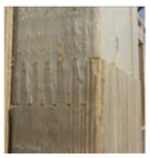
Figure 2.
Finger-jointed stud used in the residence construction.
A 20” diameter tree with 42 feet length of usable wood produces about 260 board feet (0.614 cubic meters). The Idaho Forest Products Commission estimated that a typical 2000 square foot (185.8 square meters) house would use 102 trees of that size, 19.6 trees per square foot [20]. For the simulation, there is little quantitative support about the amount of reduction achieved in construction through the use of engineered lumber. This uncertainty translated to a uniform distribution with a conservative range of 10% to 20% reduction (flexible) based on the user input on trees per square foot (defaulted to 20, flexible). Equation (1) provides the operationalization for lumber usage. In this equation, the number of trees used is a binomial mixture, where LUM is an indicator for the use of engineered lumber. The resulting equation reduces consumption by 10 to 20% uniformly when engineered lumber is selected and 0% otherwise.
The cost of finger-jointed studs may be more expensive than regular studs. At one lumber site, retail cost of a 2 × 4 × 104 5/8” regular pine stud versus the same size finger-jointed stud is listed at $3.62 [21] versus $5.59 [22], respectively. This is a 54.4% cost increase for materials, which might be offset by lower labor costs due to engineered lumber’s straightness. Engineered lumber typically results in a lowered installed cost per square unit [23].
The cost differential is not atypical, as many engineered lumber products have upcharges between 1.5 and 2 times the cost of traditional lumber [24]. A reasonable estimate for the total cost of traditional framing is between $4 to $10 per square foot for labor and $3 to $6 per square foot for materials [25]. These values were used in a uniform distribution for non-engineered lumber. Conservatively, a uniform 10% to 20% reduction in labor costs and uniform 1.5 to 2.0 times increase in material costs were used for engineered lumber calculations. Equation (2) shows the lumber cost calculations in the simulation. In this binomial mixture equation, the indicator variable LUM mixes traditional wood construction (1-LUM) with engineered wood construction (LUM). Traditional wood construction labor and material costs are modeled uniformly between $4 and $10 per square foot and between $3 and $6 per square foot, respectively. For engineered wood construction, labor costs are reduced between 10 and 20% uniformly and material costs are 1.5 to 2.0 times higher. No operations and maintenance (O&M) costs were assessed for lumber selection due to its lengthy lifespan.
2.2. Acquisition Costs of Air, Water, and Vapor Barriers
For the research house motivating this simulation, Icynene spray foam was selected over other products (e.g., fiberglass, cork, pressed straw, coconut fiberboard, etc.) as it is multipurpose, providing an air barrier, vapor barrier, and water barrier, eliminating the need for attic vents, test ductwork, or air-seal attics. Icynene is environmentally friendly, made of 100% pure water-blown air, and it contains no artificial chemicals [26]. Residential spray foam insulation (Figure 3) provides a thermal barrier with exceedingly low conductivity (0.021 W/mK in one study [27]). Spray foam has reasonable hygrothermal properties and is resistant to moisture migration. The practical relevance of the tight seal around the residence is that during the heat of the Texas summer (in excess of 100 °F), the observed temperature in the attic spaces does not exceed 80 °F/26.7 °C with the house thermometer set to 76 °F/24.4 °C. The estimated wall U-values are 0.12, while the U-values for the slab foundation (8” to 8’ on the slope) are estimated between 0.07 to 0.83. The simulation includes an Icynene spray foam option for these reasons.
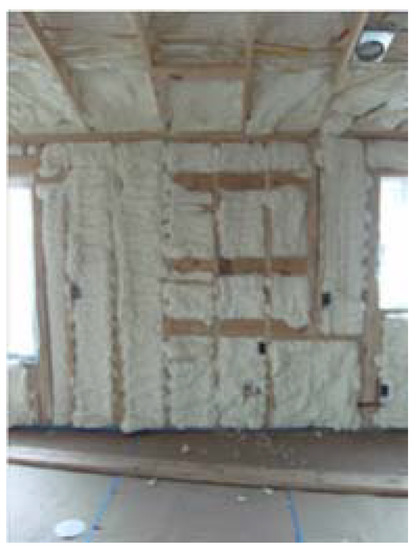
Figure 3.
Open-cell spray foam insulation installed in the residence.
The 2020 cost for open-cell spray foam insulation is about $0.35 to $0.55 per board foot [28]. Assuming 3.5” depth of spray converts to $1.23 to $1.93 per square foot, values used in the simulation of cost. Fiberglass batt insulation runs $0.64 to $1.19 per square foot (2359.17 cubic centimeters) [29]; however, this value provides an incomplete picture. Spray foam works as an air barrier, vapor barrier, water-resistant barrier, and insulation. There is no need for attic vents, test ductwork, or air-seal attics. When evaluated in this manner, it is actually 10–15% less expensive than traditional construction [30]. To account for these components when selecting non-spray foam insulation, a uniform distribution between 0.85 and 0.90 was divided by the non-spray foam insulation costs to inflate them (see Equation (3)). In this equation, the indicator variable INS is coded as 1 if Icynene foam is selected and 0 otherwise and U indicates a uniform variable on the ranges provided. No O&M costs were assigned for insulation, as all forms can last beyond 40 years.
2.3. Acquisition Costs and Selection of Windows and Doors
In the simulation, the user can select Energy Star windows and doors similar to those used in the motivating residence’s construction. The choice of windows and doors based on the solar heat gain coefficient (SHGC) is important to the home energy usage. The SHGC is defined as the fraction of incident solar radiation admitted through a window. In warm climates, windows should have solar heat gain coefficients (SHGCs) lower than 0.25 [31]. Further, the U-value, a factor that expresses the insulative value of windows, should be 0.4 or lower.
Low emissivity windows are typically 10% to 15% more expensive than standard windows [32]. The typical cost range in 2020 dollars is $385 to $785 with an average of $585 [33]. The Department of Energy (DOE) estimates savings of $125 to $465 per year from replacing windows with new windows that have higher Energy Star ratings [34]. In the simulation, Energy Star windows are modeled as a 12% reduction from kWh based on DOE estimates [34]. The simulation requests that the user specify the number of windows and doors in the house and select whether they will be Energy Star certified (checkbox). Acquisition costs are shown in Equation (4) based upon a 15% premium for Energy Star doors and windows per the Department of Energy. In this equation, ENERGY is an indicator variable indicating that Energy Star doors were installed. Doors need not be replaced during the maximum 40-year simulation, but windows are modeled as being replaced every 20 years.
2.4. Selection of Water System
The decision to install a rainwater harvesting (RWH) system versus a well or municipal water is one that is dependent on environmental considerations, the availability of municipal water, the homeowner’s wishes, and regulations. For the residence that informed the simulation, no city water sources were available, so the choice was either well or RWH. After a cost analysis, it was estimated that the acquisition costs for a well and the cost for an RWH system would be nearly identical based on well depth and rainwater design considerations. The simulation provides the user the opportunity to select rainwater, well, or municipal water options. More information about RWH system design and quality is available from these resources: [5,34,35,36].
2.4.1. Acquisition Costs of Well, Rainwater, and City Options
Acquisition costs for an RWH system (guttering, PVC piping, cistern with butyl rubber liner, and accessories) are approximately $8000 to $10,000 [37], but a large tank requirement can increase this value (e.g., $25,500 for the tank [38]). The cistern is the largest expense. The retail cost is $0.0625 per gallon for a Pioneer tank at one location [37], although it is possible to use fiberglass tanks at a less expensive rate ($0.50 per gallon) [38]. Current well drilling prices in the U.S. are between $15 and $30 per foot, up to $50 for difficult terrain [39]. For the simulation, users select the well depth or the cistern size. If city or municipal water is available, there is no acquisition cost. Equation (5) illustrates how acquisition costs were assessed. In this equation, WELL is an indicator variable for the construction of a well with an associated cost distribution (triangular) based on [39] and well depth. RWH is an indicator variable for the selection of a rainwater system with the price equal to $0.50 to $0.70 per gallon of storage. This price includes complete installation of the system (including the pump). The indicator CITY is omitted, as municipal connection fees are nominal and not charged as part of the acquisition of a water system.
2.4.2. O&M Costs for Water
Equation (6) accounts for the annual maintenance and operations of the water system selected for the simulation scenario. According to the Environmental Protection Agency (EPA), the average American uses about 88 gallons of water per day [40]. The cost of municipal water in the US is approximately $0.006 per gallon per person per day [41]. According to the Centers for Disease Control and Prevention (CDC), wells should also be inspected annually [42] at a cost of $300 to $500 per year [43]. Rainwater harvesting systems also have annual maintenance expenses. If gutter and roof cleaning is done by the owner, then the cost is estimated at $328 per year by the Environmental Protection Agency [44]. These costs are represented in Equation (6). In this equation, city water costs are based on a per gallon demand and a rate between ($0.004, $0.006) per gallon. Well O&M costs are $300 to $500 per the CDC, and RWH maintenance costs are centered around the EPA cost estimate. The accumulation rate is defined as 1 + inflation.
Selection of appliances and fixtures is important for a sustainable house reliant on 100% rainwater. Toilets, shower heads, and other water fixtures in the residence that inspired this simulation were low flow/high pressure. Mayer et al. [45] estimate that toilets use 29% of indoor water consumption, while water used for bathing, dishwashing, and laundry consume about 36%, 14%, and 21%, respectively. The Environmental Protection Agency (EPA) shows that high pressure, low flow shower heads reduce flow from 2.5 gallons per minute to 2.0 gallons per minute, a 20% reduction [46]. The Department of Energy estimates water savings between 25% and 60% [47] (values used in the simulation). Costs for low flow fixtures are comparable to standard fixtures, so acquisition costs were omitted. Equation (7) is the water demand. In this equation, LOW is an indicator variable for installation of low flow devices, and the mixture equation includes a uniform reduction of 25% to 60% if those fixtures are installed.
2.4.3. Acquisition, Replacements Costs, and Environmental Considerations Based on Selection of Water Heater, Adjusted Water Demand
One of the simulation options is tankless electric water heaters. These water heaters take up less space than those with tanks and do not constantly use energy to keep water warm. One study indicated that the life cycle savings over traditional electric storage systems is 3719 Australian dollars (about $2500 US dollars) [48]. However, that study does not consider the possibility that all electrical power needed is generated by solar. Further, the carbon footprint is much lower, as it is in operation only when demanded. Tankless water heaters may be as much as 99% efficient [38], saving 27% to 50% of kWh consumption [49]. The acquisition cost of an electric tankless heater is largely dependent on size, capability, and brand and may be higher than traditional tank versions; however, many high capacity electric versions are comparable in acquisition costs with traditional tank versions. Tankless may also last 1.5 to 2 times as long as tank water heaters (20 years) and save 8% to 34% on water (values used in the simulation), depending on water demand; however, demand flow for multiple simultaneous operations must be evaluated and proper capability systems selected [50]. The water demand reduction factor was included in the simulation by a uniform distribution between 0.66 and 0.92 as shown in Equation (8). Acquisition and replacement costs for tankless and tanked water heaters were based on user input for average cost (inflation-adjusted), while the replacement life was estimated at 8–10 years (uniform distribution) for tanked heaters and 15–20 years (also uniformly distributed) for tankless [51].
2.4.4. Environmental Consideration: Water Supply Requirements for Meeting Residents’ Water Demand
For the simulation, users select from RWH, well, or city/municipal water sources. From a sustainability perspective, RWH requires far less water for the same aquifer demand (either well or municipal). Specifically, run-off, absorption and adsorption, and evaporation and transpiration reduce aquifer resupply to about 30% [52]. On the other hand, RWH systems capture 75% to 90% of rainwater, depending on design and rainfall [35]. The amount of water pulled from the aquifer to supply one gallon is therefore at 2.5 to 3.0 times as much as rainwater harvesting. Equation (9) illustrates how the simulation accounts for the water supply requirements to satisfy demand. RWH is an indicator variable indicating a rainwater harvesting system. This equation is adjusted later for selection of low flow devices and installation of tankless water heaters.
2.5. Acquisition, O&M Costs, and Environmental Considerations for Waste Management System
Cradle-to-grave water management requires that black water be treated responsibly and sustainably. Traditional municipal waste management and septic systems (aerobic and anaerobic) are two options for treating waste at residences, while traditional wastewater treatment plants are a third option. All three are available in the simulation.
Unlike traditional anaerobic septic fields, Biologically Accelerated Treatment (BAT) plants (also termed Biologically Accelerated Wastewater Treatment (BAWT) plant) work by treating wastewater physically and biologically in a pre-treatment compartment. Water then flows through the treatment compartment where it is aerated, mixed, and treated by a host of biological organisms (a biomass). The mixture then flows to a settlement compartment where particulate matter settles, returning to the treatment compartment, leaving only odorless and clear liquid (gray water produced by the biomass) which is discharged through sprinkler heads [53]. Figure 4 is an encased BAT system. Aerobic systems break down waste far quicker than anaerobic due to the nature of the bacteria.
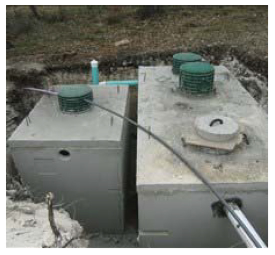
Figure 4.
Biologically Accelerated Treatment plant during installation at research residence.
Installing a typical anaerobic system averages $3500, whereas an aerobic costs about $10,500 [54]. Maintaining the aerobic septic system is about $200 annually [55], which is somewhat more than anaerobic systems [56] (modeled as 50% of the cost on average). There are benefits to the environment in that (1) pumps for transporting water to wastewater treatment plants are not necessary (and the associated energy costs), (2) treated water returned to the environment is cleaner, (3) electricity for processing water (in this case) is largely if not entirely generated by the sun. Equations (10) and (11) are the acquisition and operation costs for the simulation. In these equations, AEROBIC is an indicator variable for an aerobic septic system, ANAEROBIC indicates an anaerobic septic, and city waste management is omitted (zero cost and nominal O&M).
2.6. Acquisition/O&M Costs, Electrical Systems
For the simulation, users are asked to select the percent of kWh provided by solar. Acquisition of a system includes extra capacity to account for 0.004% decay per year. In doing so, O&M costs for the duration of the simulation are built-in [57]. To illustrate, a 30-year horizon would require 11.33% more panels. Further, users were required to select their state, as geography has an impact on capture. That impact was acquired by evaluating the ratio of the recommended photovoltaic system size recommended by manufacturers to the kWh used monthly (e.g., [58]). Cost per solar panel watt was a user option, set between $2 and $5 with the default value of $3.18 [59]. Equation (12) is the solar acquisition cost when selected, where SOLAR is an indicator variable for the inclusion of a solar system, ENERGY is an indicator variable for Energy Star windows/doors.
O&M costs for solar are negligible, particularly since the decay factor is included in the system [60]. Residential electricity rates are anticipated to be fairly stable over time as well [61]. For the simulation, the user inputs the initial cents per kWh, which are inflated over time based on the anticipated electrical inflation rate. Equation (13) provides the electrical O&M costs for the simulation. The total kWh is calculated later.
From an environmental perspective, the carbon dioxide avoidance by leveraging solar is significant. The footprint of solar is 6 g CO2e/kWh, while coal carbon capture and storage (CCS) is 109 g and bioenergy is 98 g. Wind power produces lower emissions (4 g); however, the research residence location is a low-production wind area [62]. Wind power will be incorporated in a future version of the simulation. Equation (14) is the CO2e/kWh formula used in the simulation. This equation includes a calculation for gasoline cars of 8887 grams per gallon of gas consumed [63]. An inherent assumption of this formula is that the percentage offset by solar is a true offset, not just credited.
2.7. Acquisition/O&M for Vehicle (Important for EV Considerations)
Electricity generated from solar panels may be used to charge electric vehicles (Figure 5). A low-end electrical vehicle such as a Nissan Leaf 8-year costs are estimated to be $36,537.82 with total 8-year energy costs (kWh) at $3969 [64]. When powered by solar that is 100% capable of producing both home and automobile power, there are negligible O&M energy costs. Thus, the difference in cost between an equal value gasoline car (after accounting for any tax credits and residual) would be the maintenance and energy costs. In the simulation, the user selects the car acquisition cost for comparison (possibly zero to omit this element). Equation (15) reflects the implementation of the comparison in the simulation if a user selects an electric vehicle. The last portion of the equation uses the complement of the indicator for electric vehicles (EVs) and multiplies that by the annual cost of driving. The user selects the starting gasoline cost (inflated), miles driven, and miles per gallon.
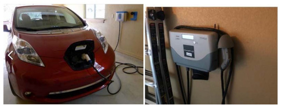
Figure 5.
Nissan Leaf and charging station installed at research residence.
2.8. Acquisition Costs for Heating, Ventilation, and Air Conditioning
As part of the research construction, the residence was equipped with a closed loop, geothermal system (see Figure 6). This became an option in the simulation. Vertical, closed-loop geothermal units are heat exchangers that leverage the fact the temperature 200’ below the Earth remains relatively constant. The cost of the system including wells, unit, and ducting (complete) was $26,500. The tax credit currently stands at 30%. Climatemaster (the brand installed) estimates a $1000 savings in electrical costs per year over an electric heat pump ($3135 versus $4169) [65].
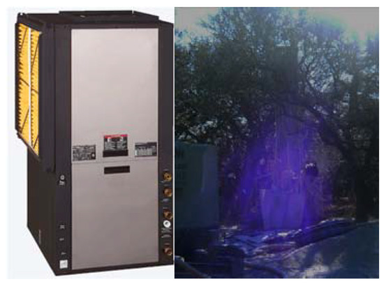
Figure 6.
Geothermal unit and vertical drilling of wells.
Acquisition costs for geothermal are much more than traditional heat pumps [66]. In the simulation, the user selects the tonnage required, and this tonnage is used to estimate the total install cost. Equation (16) illustrates the simulation implementation, where GEO is an indicator variable for the installation of a geothermal system.
Geothermal systems may be more expensive but reduce kWh usage. This reduction is factored into the total kWh calculation in Equation (17) along with Energy Star windows and doors, tankless water heaters, and electric vehicle consumption. ENERGY, GEO, TANKLESS, and EV are indicator variables for the presence of Energy Star doors/windows, geothermal heating, tankless water heaters, and an electric vehicle, respectively.
2.9. Simulation Runs and Flowchart
The number of simulation iterations is user-specified from 1000 to 8000. A confidence interval of 95% is graphed across the break-even graph for users to evaluate the variability of the estimates. The default value is 2000 iterations. Figure 7 is the flowchart with red text indicating the step identifier for discussion. While the equations were explicated earlier, a detailed discussion follows.
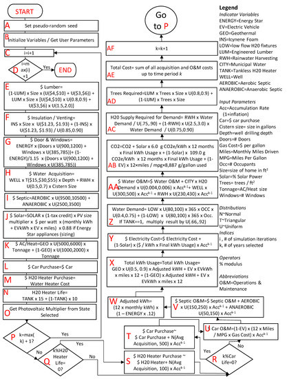
Figure 7.
Flowchart for the simulation with red text identifying steps.
The flowchart starts in the upper left (step START), and a common random number seed (step A) is set for comparison across models. Step B initializes all variables and retrieves parameters from the user interface for use in the simulation. In step C, the number of simulation iterations indexed by i is incremented by 1. While i is less than the maximum number of iterations +1 (originally set by the user in the user interface with values between 1000 and 8000), the simulation continues to step D, otherwise, it terminates (step END).
Next, acquisition costs are assigned. These costs include lumber (step E), insulation/venting (step F), doors and windows (step G), water acquisition (as needed, step H), septic (step I), solar (step J), HVAC system (step K), vehicle acquisition costs (if desired to compare electrical versus non-electrical, step L), and water heater acquisition (step M). Additionally, water heater life (step N) and the state photovoltaic multiplier (step O) are obtained [58]. These elements are included in the left-hand column on the flowchart. At the bottom of this column, iterations for the number of years (user selected up to 40 and indexed as k) begin (step P).
After acquisition costs, the simulation estimates replacement costs for certain major items. Each year, there are checks for water heater replacement (step Q) and vehicle replacement (acquisition costs, step R) based on estimated lifespan. If required, these costs are introduced (step S and T, respectively). Otherwise, annual vehicle costs (step U) are calculated directly.
Operations and maintenance costs, as well as environmental effects, are then estimated. Annual septic costs are calculated (step V) followed by consumption of kWh per year based on Energy Star or no Energy Star appliances (step W). This calculation is then adjusted in step X for user selection of geothermal and electric vehicles. In step Y, the kWh consumption is converted to costs. Annual water demanded for the residence is then calculated based on occupancy, selection of low flow appliances by the user, and supply method (well, rainwater, municipal) in step Z. In step AA, the user selections for the water system are converted to operations and maintenance costs for the water system. Step AB estimates the CO2 emissions for the selected electrical source, percent solar acquisition, and usage of vehicle (electric or otherwise) based on user input from the simulation. In step AC, the actual water required to meet the demand is calculated, and in step AD, the number of trees required for the building construction is estimated. In step AE, all acquisition and discretionary costs are aggregated for the iteration. Finally, step AF increments the years for the analysis and sends the simulation back to step P.
2.10. Verification and Validation (V&V)
Since the simulation was written in R Shiny, several methods were available for verification and validation. To investigate validity, prior and posterior distributions were investigated to ensure that output distributions matched the input distributions. For validity across experimental conditions, a common random number stream was used. In doing so, we ensured that comparison differences would not be due to the selection of pseudo-random numbers alone. Third, visualization of the simulation results ensured that the outcomes were as expected.
3. Results
3.1. Baseline vs. Scenario 1
The baseline scenario was set to include the parameters in Figure 8. Runs were based on 30-year ownership, 3000 square feet construction (279 square meters), 25 windows, 3 external doors, 2 occupants, 2 water heaters, $1000 water heater acquisition, 30% tax credit, 5 ton (4.5 metric ton) heat pump/geothermal heat pump in Texas, 1500 base kWh usage per month, $0.13 per kWh utility costs, $3.30 per watt solar panels, 3% annual inflation, 0.3 kWh per mile for EV, $30,000 base cost for vehicles, 1100 monthly miles, 30 mpg for gas vehicles, $2.20 per gallon for gasoline, 8-year car life, and 2000 simulation runs. Comparative construction analysis in Figure 8 included all possible sustainable checkboxes offered in the simulation plus rainwater harvesting and an aerobic septic system, mimicking the research residence.
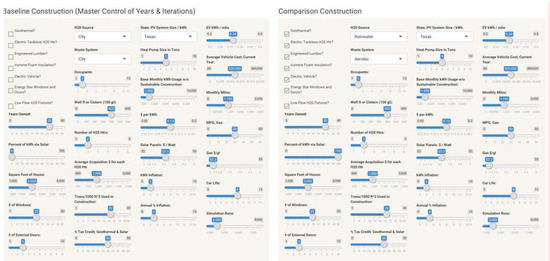
Figure 8.
Baseline and comparison construction information, Scenario 1.
3.1.1. Scenario 1—All Sustainable Items Checked
Figure 9 shows the graphical results of the break-even analysis for Scenario 1. The break-even time based on this analysis is about 23 years due to the up-front expenses. At 30 years, the cost savings are estimated to be $50,000. The sustainable construction option saves 60,736 kilograms of CO2 (Equation (14)) and requires 5495 fewer kilogallons of water to meet demand over the 30-year lifespan. The sustainable option requires 201 fewer MWh over the course of 30 years, and the grid cost is zero as solar provides 100% of the power required. While better for the environment, water and wastewater are more expensive for sustainable construction and can never achieve any break-even. An inherent assumption and limitation with this scenario is that a 100% solar option provides sufficient electricity for the household without the additional need for grey electricity. In other words, the home has sufficient storage such that it consumes no power from the grid day or night.
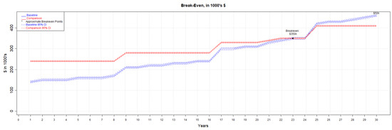
Figure 9.
Break-even analysis for Scenario 1.
3.1.2. Scenario 2—100% Solar Only
Scenario 2 includes 100% solar as the comparison option. Break-even is at nine years with the maximum cost savings at 30 years equal to $100,000. See the comparison in Figure 10. CO2e savings over traditional construction totals 55,620 kilograms. If tax credits are reduced to zero, then the break-even moves to 13 years rather than 9.
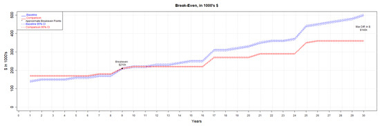
Figure 10.
100% solar versus the baseline.
3.1.3. Comparison Tables for Various Scenarios
The number of scenarios available is beyond enumeration, as the simulation is designed to support user input. Thus, the design of experiments and response surface methodology are outside the scope. Given the fixed parameters for the baseline discussed previously, comparison changes were made for many of the sustainable construction options. Interestingly, Icynene foam and engineered lumber are not major contributors to the cost or break-even analysis. The hypothetical advantage of EVs is offset by the requirement for more solar in a 100% solar solution, as well as gas prices. Other combinations are left to the user to explore. Table 1 illustrates the results.

Table 1.
Comparison of simulation break-even results.
4. Discussion
The simulation results show that building a sustainable house can be both green for the environment and green for the pocketbook depending on the trade-off considerations of the consumer. The simulation results show that many but not all sustainable construction options have an associated cost premium up front. The initial up-front costs may be quickly offset by savings depending on construction options. Of importance, we note that a 100% solar solution alone offsets the acquisition costs for the baseline construction in about 9 years with 30% tax credits.
Some construction elements showed no cost–benefit. For example, an aerobic septic system has both higher acquisition costs and higher maintenance costs than an equivalently sized anaerobic system. The use of engineered lumber or Icynene foam does not produce measurable cost benefits, although engineered lumber reduces the number of trees required and is environmentally responsible. An electric car without any associated solar power offset may actually cost the homeowner more, depending on the gas prices versus the kWh electrical prices; however, the CO2 admissions are reduced. Even rainwater harvesting requires more acquisition, operations, and maintenance costs than well or city water but reduces the total water required for each gallon demanded.
Aside from the economic considerations, there are environmental considerations. The amount of CO2 produced in electrical consumption through coal-powered plants is multiple times that of solar (109 grams versus 6 grams per kWh). Further, the amount of water required to produce a single gallon for consumption is significantly reduced by rainwater harvesting. Low flow appliances also reduce consumption and are of similar cost to more wasteful appliances.
In evaluating the two scenarios presented, both achieved break-even and reduced environmental impact. Scenario 1 (all sustainable options checked) saved over 60,000 kilograms of CO2, a non-trivial amount, and required nearly 5500 fewer kilogallons of water to meet demand over the 30-year lifespan. The consumer, however, would not experience a break-even until year 23. An all solar scenario, however, had a quick break-even of 9 years and still saved nearly 56,000 kilograms of CO2. Both of these scenarios illustrate that green construction may be green for the pocketbook as well.
4.1. Policy Considerations
There are also policy requirements for sustainable construction. For example, California now requires new residential construction to offset its own electrical demand. This mandate is one aspect of the California Energy Commission’s initiative to have 50% of the entire State of California’s energy production be from a clean energy source by 2030 [67]. Another law restricts California residents to 55 gallons/day water usage by 2022 and 50 gallons/day by 2030 [68]. Mandates on both electric and water usage are likely the wave of the future. A proactive approach leveraging the analysis presented here and elsewhere will help both builders and buyers.
4.2. Limitations
The limitations of the simulation in this study are significant. First, only a limited subset of sustainable and non-sustainable construction components is considered. Many others will be added in future work, but modeling the universe is not realistic. Second, the estimates in this study are based on evidence and professional assessment; however, they may contain more errors than modeled. Third, the distributions selected, while ostensibly reasonable, may be improved with additional analysis. Finally, it is important to note that a 100% solar option assumes that no grey electricity is consumed (i.e., there is solar power storage).
4.3. Future Sustainable Improvements and Modeling
All add-on construction to the residence included mini-splits (both in wall and in roof systems). These systems have more upfront costs but are much more energy efficient, as they do not lose energy through ductwork. Further, they are now inconspicuous and highly effective [69]. See Figure 11 for pictures of in-roof and in-wall systems installed in the residence. In new construction, these systems should be considered due to their efficiency and elimination of ductwork and other requirements.
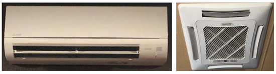
Figure 11.
Mini-split units mounted in research residence, wall and roof versions.
Another new construction consideration is the use of wireless multi-gang light switches. These fixtures can minimize wiring requirements by using a single drop instead of multiple drops. With the advent of 5G, it might be possible to eliminate CAT6 wiring during residential construction in the future as well.
This is the first simulation of its type that quantifies multiple sustainable construction options, associated break-even points, and environmental considerations. In future simulations, wind power, as well as natural gas and propane, will be modeled. Distributions and parameters will be refined where possible, and additional input options for users will appear.
5. Conclusions
The primary hypothesis in this study was that some elements of green construction might also be green for the pocketbook. The simulation demonstrates that break-even is achievable for many combinations of sustainable construction components but not for each possible combination. As legislation and best-practice construction methods increasingly push towards sustainable interventions, knowledge of the environmental and consumer costs is necessary. This publicly available simulation, the first of its type, addresses this analysis requirement.
Author Contributions
Conceptualization, L.F.; methodology, L.F. and B.B.; validation, L.F.; programming, C.K. and M.B.; formal analysis, L.F., B.B., and M.B.; writing, L.F., B.B., M.B., and K.L.; and review, C.S.K. All authors have read and agreed to the published version of the manuscript.
Funding
This research received no external funding.
Conflicts of Interest
The authors declare no conflict of interest.
References
- Yale Environmental Review. Available online: https://environment-review.yale.edu/reducing-environmental-impact-green-buildings-0 (accessed on 2 January 2020).
- Suh, S.; Tomar, S.; Leighton, M.; Kneifel, J. Environmental Performance of Green Building Code and Certification. Environ. Sci. Technol. 2014, 48, 2551–2560. [Google Scholar] [CrossRef] [PubMed]
- Jain, M.; Hoppe, T.; Bressers, H. A governance perspective on net zero energy building niche development in India: The case of New Delhi. Energies 2017, 10, 1144. [Google Scholar] [CrossRef]
- The ‘Greenest’ Home in Texas. Available online: https://www.ksat.com/weather/2012/02/09/the-greenest-home-in-texas/ (accessed on 2 January 2020).
- Fulton, L.V.; Bastian, N.; Mendez, F.; Musal, R. Rainwater Harvesting System Simulation using a Non-Parametric Stochastic Rainfall Generator. Simulation 2013, 89, 693–702. [Google Scholar] [CrossRef]
- Fulton, L.V. A Simulation of Rainwater Harvesting Design and Demand-Side Controls for Large Hospitals. Sustainability 2018, 10, 1659. [Google Scholar] [CrossRef]
- Meron, N.; Meir, I. Building green schools in Israel. Costs, economic benefits and teacher satisfaction. Energy Build. 2017, 154, 12–18. [Google Scholar] [CrossRef]
- Yeganeh, A.J.; McCoy, A.P.; McCoy, S. Green affordable housing: Cost-benefit analysis for zoning incentives. Sustainability 2019, 11, 6269. [Google Scholar] [CrossRef]
- Sun, C.; Chen, Y.G.; Wang, R.J.; Lo, S.C.; Yau, J.T.; Wu, Y.W. Construction cost of green building certified residence: A case study in Taiwan. Sustainability 2019, 11, 2195. [Google Scholar] [CrossRef]
- Dwaikat, L.; Ali, K. Green buildings cost premium: A review of empirical evidence. Energy Build. 2016, 110, 396–403. [Google Scholar] [CrossRef]
- Liu, Y.; Guo, X.; Hu, F. Cost-benefit analysis on green building energy efficiency technology application: A case in China. Energy Build. 2014, 82, 37–46. [Google Scholar] [CrossRef]
- Liu, L.; Liu, C. The economics of sustainable residential building in Australia. In Proceedings of the 6th International Conference on Machinery, Materials, Environment, Biotechnology and Computer (MMEBC 2016), Tianjin, China, 11–12 June 2016; Available online: https://www.atlantis-press.com/proceedings/mmebc-16/25859006 (accessed on 19 March 2020).
- Ade, R.; Rehm, M. Buying limes but getting lemons: Cost-benefit analysis of residential green buildings—A New Zealand case study. Energy Build. 2019, 186, 284–296. [Google Scholar] [CrossRef]
- Fulton, L.; Beauvais, B.; Brooks, M.; Kruse, C.S.; Lee, K. Green for the environment and green for the pocketbook: A decade of living sustainably. Preprints 2020, 2020020002. Available online: https://www.preprints.org/manuscript/202002.0002/v1 (accessed on 19 March 2020). [CrossRef]
- Penn, I. California Will Require Solar Power for New Homes. New York Times. 8 May 2018. Available online: https://www.nytimes.com/2018/05/09/business/energy-environment/california-solar-power.html (accessed on 1 April 2020).
- Glaeser, E.L.; Gyourko, J. The impact of building restrictions on housing affordability. Econ. Policy Rev. 2003, 9, 1–19. [Google Scholar]
- Chang, W.; Cheng, J.; Allaire, J.J.; Xie, Y.; Mcpherson, J. Shiny: Web Application Framework for R. R Package Version 1.4.0. 2019. Available online: https://CRAN.R-project.org/package=shiny (accessed on 25 February 2020).
- Google Maps Imagery@2020 CAPCOG Maxar Technologies. Available online: https://www.google.com/maps/@29.7772101,-98.3875654,140a,35y,163.01h,8.72t/data=!3m1!1e3 (accessed on 2 January 2020).
- De Silva, S.; Liyanage, V. Suitability of finger jointed structural timber for construction. J. Struct. Eng. Appl. Mech. 2019, 2, 131–142. [Google Scholar] [CrossRef]
- McMansions Are Not Eco-Friendly. The Seattle Times. Available online: https://www.seattletimes.com/business/real-estate/mcmansions-are-not-eco-friendly/ (accessed on 2 January 2020).
- Menards 2 × 4 × 104 5/8’’ Pre-Cut Stud Construction/Framing Lumber. Available online: https://www.menards.com/main/building-materials/lumber-boards/dimensional-lumber/2-x-4-pre-cut-stud-construction-framing-lumber/1021091/building-materials/lumber-boards/dimensional-lumber/2-x-4-pre-cut-stud-construction-framing-lumber/1021305/p-1444422686698.htm (accessed on 2 January 2020).
- Menards 2 × 4 × 104 5/8’’ Finger Joint Pre-Cut Stud Construction/Framing Lumber. Available online: https://www.menards.com/main/building-materials/lumber-boards/dimensional-lumber/2-x-4-finger-joint-pre-cut-stud-construction-framing-lumber/1021111/p-1444422419687.htm (accessed on 2 January 2020).
- Probuilder. Available online: https://www.probuilder.com/wood-vs-engineered-lumber (accessed on 8 March 2020).
- The Pros and Cons of Engineered Lumber. Available online: https://www.residentialproductsonline.com/pros-and-cons-engineered-lumber (accessed on 2 January 2020).
- How Much Does It Cost to Frame a House? Available online: https://www.homeadvisor.com/cost/walls-and-ceilings/install-carpentry-framing/ (accessed on 2 January 2020).
- Sustainability and Green Innovation Easy with Icynene Spray Foam Insulation. Available online: https://www.icynene.com/en-us/news/sustainability-and-green-innovation-easy-icynene-spray-foam-insulation (accessed on 11 February 2020).
- Li, Y.; Yu, H.; Sharmin, T.; Awad, H.; Gull, M. Towards energy-Efficient homes: Evaluating the hygrothermal performance of different wall assemblies through long-term field monitoring. Energy Build. 2016, 121, 43–56. [Google Scholar] [CrossRef]
- How Much Does It Cost to Insulate a House? Available online: https://www.homeadvisor.com/cost/insulation/ (accessed on 2 January 2020).
- Foam Insulation vs. Fiberglass, Cellulose: Which Is the Right Choice? Available online: https://www.probuilder.com/insulation-choices-fiberglass-cellulose-or-foam (accessed on 2 January 2020).
- What Makes It Energy Star? Available online: https://www.energystar.gov/products/building_products/residential_windows_doors_and_skylights/key_product_criteria (accessed on 2 January 2020).
- Homebuilders Uing Low-E Windows to Reduce Energy Costs. Available online: https://www.thebalancesmb.com/uses-of-low-e-windows-844755 (accessed on 2 January 2020).
- How Much Do Energy Efficient Windows Cost? Available online: https://modernize.com/windows/energy-efficient (accessed on 2 January 2020).
- Benefits of Energy Star Qualified Windows, Doors, and Skylights. Available online: https://www.energystar.gov/products/building_products/residential_windows_doors_and_skylights/benefits (accessed on 2 January 2020).
- US Department of Energy Energy Star Qualified Windows. Available online: https://www.energystar.gov/ia/partners/manuf_res/downloads/PartnerResourceGuide-LowRes.pdf (accessed on 8 March 2020).
- Texas Water Development Board. Texas Manual on Rainwater Harvesting, 3rd ed.; State of Texas: Austin, TX, USA, 2005; p. 30. [Google Scholar]
- Fulton, L.; Muzaffer, R.; Mendez Mediavilla, F. Construction analysis of rainwater harvesting systems. In Proceedings of the 2012 Winter Simulation Conference (WSC), Berlin, Germany, 9–12 December 2012. [Google Scholar] [CrossRef]
- Texas Co-op Power Rainwater Harvesting FAQ. Available online: https://www.texascooppower.com/texas-stories/life-arts/rainwater-harvesting-faq (accessed on 2 January 2020).
- Rain Ranchers. Available online: https://rainranchers.com/above-ground-rainwater-collection-tanks/ (accessed on 8 March 2020).
- How Much Does It Cost to Drill or Dig a Well? Available online: https://www.homeadvisor.com/cost/landscape/drill-a-well/ (accessed on 2 January 2020).
- Understanding Your Water Bill. Available online: https://www.epa.gov/watersense/understanding-your-water-bill (accessed on 8 March 2020).
- Average Residential Monthly Cost of Water. Available online: https://www.statista.com/statistics/720418/average-monthly-cost-of-water-in-the-us/ (accessed on 8 March 2020).
- Well Maintenance. Available online: https://www.cdc.gov/healthywater/drinking/private/wells/maintenance.html (accessed on 2 January 2020).
- How Much Does a Well Inspection Cost? Available online: https://www.thumbtack.com/p/well-inspection-cost (accessed on 2 January 2020).
- Rainwater Harvesting. Available online: https://www.epa.gov/sites/production/files/2015-11/documents/rainharvesting.pdf (accessed on 8 March 2020).
- Mayer, P.W.; DeOreo, W.B.; Optiz, E.M.; Kiefer, J.C.; Davis, W.Y.; Dziegielewski, B.; Nelson, O.J. Residential End Users of Water; AWWA Research Foundation and American Water Works Association: Denver, CO, USA, 1999; Available online: https://www.waterrf.org/research/projects/residential-commercial-and-institutional-end-uses-water (accessed on 2 January 2020).
- EPA Showerheads. Available online: https://www.epa.gov/watersense/showerheads (accessed on 2 January 2020).
- Reduce Hot Water Use for Energy Savings. Available online: https://www.energy.gov/energysaver/water-heating/reduce-hot-water-use-energy-savings (accessed on 26 February 2020).
- Kumar, N.M.; Mathew, M. Comparative life-cycle cost and GHG emission analysis of five different water heating systems for residential buildings in Australia. Beni Suef. Univ. J. Basic Appl. Sci. 2018, 7, 748–751. [Google Scholar] [CrossRef]
- Tankless Hot Water Heaters Versus Tank Water Heaters. Available online: https://www.petro.com/resource-center/tankless-hot-water-heaters-vs-tank-storage-water-heaters (accessed on 8 March 2020).
- Tankless or Demand-Type Water Heaters. Energy Gov. Available online: https://www.energy.gov/energysaver/heat-and-cool/water-heating/tankless-or-demand-type-water-heaters (accessed on 2 January 2020).
- 3 Environmental and Economic Benefits of Tankless Water Heaters. Available online: http://www.eemax.com/2016/01/11/3-environmental-and-economic-benefits-of-tankless-water-heaters/ (accessed on 2 January 2020).
- Rain and Precipitation. USGS. Available online: https://www.usgs.gov/special-topic/water-science-school/science/rain-and-precipitation?qt-science_center_objects=0#qt-science_center_objects (accessed on 2 January 2020).
- Jet Aeration System. Available online: https://www.jetprecast.com/jet-aeration-system.html (accessed on 2 January 2020).
- New Septic System Installation Costs. Available online: https://homeguide.com/costs/septic-tank-system-cost#new (accessed on 2 January 2020).
- Compare Aerobic vs. Anaerobic Septic System Costs. Available online: https://www.kompareit.com/homeandgarden/plumbing-compare-aerobic-vs-anaerobic-septic-system.html (accessed on 2 January 2020).
- Basics for Septic Systems. Texas Commission on Environmental Quality. Available online: https://www.tceq.texas.gov/assistance/water/fyiossfs.html (accessed on 2 January 2020).
- What Is the Lifespan of a Solar Panel? Engineering.com. Available online: https://www.engineering.com/3DPrinting/3DPrintingArticles/ArticleID/7475/What-Is-the-Lifespan-of-a-Solar-Panel.aspx (accessed on 4 January 2020).
- How Many Solar Panels do I Need? Available online: https://www.gogreensolar.com/pages/how-many-solar-panels-do-i-need (accessed on 8 March 2020).
- How Much Do Solar Panels Cost to Install for the Average House in the US in 2020? Available online: https://www.solarreviews.com/solar-panels/solar-panel-cost/ (accessed on 8 March 2020).
- Solar Panels Lifetime Productivity and Maintenance. Available online: https://www.bostonsolar.us/solar-blog-resource-center/blog/solar-panels-lifetime-productivity-and-maintenance-costs/ (accessed on 8 March 2020).
- Projection of Average End-Use Electricity Price in the US from 2019 to 2050 (in US Cents per Kilowatt Hour). Available online: https://www.statista.com/statistics/630136/projection-of-electricity-prices-in-the-us/ (accessed on 20 January 2020).
- Pehl, M.; Arveson, A.; Humpenoder, F.; Popp, A.; Luderer, H.; Luderer, H. Understanding future emissions from low-carbon power systems by integration of life-cycle assessment and integrated energy modelling. Nat. Energy 2017, 2, 939–994. [Google Scholar] [CrossRef]
- Greenhouse Gas Emissions from a Typical Passenger Vehicle. Available online: https://www.epa.gov/greenvehicles/greenhouse-gas-emissions-typical-passenger-vehicle (accessed on 8 March 2020).
- Fulton, L. Ownership cost comparison of battery electric and non-plug-in hybrid vehicles: A consumer perspective. Appl. Sci. 2018, 8, 1487. [Google Scholar]
- Geothermal Savings Cost Calculator. Available online: https://www.climatemaster.com/residential/geothermal-savings-calculator/sc01.php (accessed on 2 January 2020).
- How Much Does a Heat Pump Cost? Available online: https://www.homeadvisor.com/cost/heating-and-cooling/install-a-heat-pump/ (accessed on 8 March 2020).
- California Becomes 1st State to Require Solar Panels on New Homes. Here’s How It Will Reduce Utility Costs. Available online: https://fortune.com/2018/12/06/california-solar-panels-new-homes/ (accessed on 2 January 2020).
- Brown, J.; Bee, S. Get Ready to Save Water: Permanent California Restrictions Approved by Gov. Available online: https://www.sacbee.com/news/politics-government/capitol-alert/article211333594.html (accessed on 2 January 2020).
- Mini-Split Heat Pumps: The Advantages and Disadvantages of Ductless Heating. Available online: https://learn.compactappliance.com/mini-split-heat-pumps/ (accessed on 2 January 2020).
© 2020 by the authors. Licensee MDPI, Basel, Switzerland. This article is an open access article distributed under the terms and conditions of the Creative Commons Attribution (CC BY) license (http://creativecommons.org/licenses/by/4.0/).