Improving the Efficiency and Sustainability of Power Systems Using Distributed Power Factor Correction Methods

Abstract

For the equipment connected to the three-phase or single-phase grid, the power factor represents an efficiency measure for the usage of electrical energy. The power factor improvement through correction methods reduces the load on the transformers and power conductors, leading to a reduction of losses in the mains power supply and a sustainable grid system. The implications at the financial level are also important. An example of load that generates a small power factor is represented by a motor without mechanical load or having a small mechanical load. Given the power factor correction (PFC), the costs are reduced through the elimination of penalties, applying only in the common coupling point (CCP). The advantages of using equipment for the power factor correction are related also to their long operation duration and the easiness of their installation. The device presented in this article takes advantage of the advances in information and communication technology (ICT) to create a new approach for telemetry and remote configuration of a PFC. This approach has flexibility and versatility, such that it can be adapted to many loads, easily changing the capacitance steps and settings of the power factor correction device.

1. Introduction

The power factor is a measure of the efficiency of the use of electricity. Improved power factor correction reduces the load of the transformers and conductors of electrical installations. The implications are also financial in nature, a low power factor increasing the cost of consumed electrical energy [1,2,3,4].

Reactive power is an important parameter of the electrical power that leads to a decreased power factor. It is generated by two main factors: reactive elements and unbalances in the three-phase systems [5]. For example, AC rotary machines will induce extra losses when unbalanced load current and reactive power are absorbed by a single-phase load. Sensitive electronic equipment is particularly disturbed by the low power factor generated by unbalanced current. There are many authors that explored ways to reduce the extra costs generated by reactive power [6,7,8,9,10,11].

The use of capacitors for the correction of the power factor is related to the long service life and the ease of installation. It should be kept in mind that the capacitor batteries introduce disturbances in the network when they are connected and disconnected. The maximum value of the voltage does not exceed (in the absence of harmonics) twice the maximum value of the rated voltage, when switching the discharged capacitors [12].

In the case of a capacitor already charged at the time of switching off, the overvoltage can reach a maximum value approaching three times the peak nominal value. When considering the automatic step change of capacitor batteries, care must be taken that the section of capacitors to be supplied is completely discharged [1,12].

An overexcited synchronous condenser is another option to correct the power factor. Basically, it is a synchronous electric drive/generator in the no load electric drive state, but with overexcited current. This is a much more expensive option because of the special design needed (e.g., oversized windings and special rotor shaft), which is the main disadvantage. An advantage is the missing disturbances in the power network.

Good management of an electrical energy consumer network includes the evaluation of the power factor and actions to improve it. For the reliable measurement of power, reactive power, the appearance of the resonance phenomenon needs to be taken into consideration and has been studied by various authors, with several approaches being published in various articles [13,14,15]. We use mathematical models to describe the performance of the power factor corrector, similar to the ones described in [16]. There are also principles for optimization of the power factor in a closed network, such as the proportional-integral-derivative (PID) algorithm [17].

In the context of increasing the penetration of the intermittent renewable energy sources, the concept of microgrids (MG) becomes more frequent as a solution to these issues. There are efforts being made to improve the solutions available to microgrid developers in order to compensate the power factor and the load asymmetries inside the microgrid by utilizing advanced functionalities enabled by grid tied inverters of photovoltaics and energy storage systems [18,19].

Advanced operational capabilities of power electronic based distributed energy resources (DERs) can be employed to compensate power quality phenomena such as harmonics, interharmonics, and current/voltage unbalances [15,19,20,21,22]. Hence, smart and multi-functional inverters are capable of providing multiple ancillary services to the MG, along with dedicated resources such as automatic power factor correction equipment.

The problems of degrading power factor and reactive power are mainly present in the industrial environment, where the frequency of inductive loads is significant, most commonly from electric motors. Due to rapid advances in ICT, the digital transformation is expanding across all domains. In the industrial environment, most often, it takes the form of Industry 4.0 ecosystems that integrate several technologies and concepts such as the Internet of Things (IOT), big data, cloud computing, and smart metering, in order to allow real-time monitoring and controlling of a complex industrial system using remote computers and mobile devices [23,24,25,26,27].

Similar applications are employed in ship main propulsion power monitoring systems. In the particular application explored in [28], wireless telemetry technology was used alongside the MODBUS communication protocol.

The topic of power factor correction has been previously explored and presented in the literature, using different approaches. In [29], a new digital power factor correction (PFC) control strategy was presented, based on digital signal processor speed to solve the problem of limited switching frequency. In [30], a programmable logic controller (PLC) was used to control switch capacitors for PFC near a three-phase electric induction motor. More complex PFC decision algorithms were analyzed in [31], and a new teaching learning based optimization (TLBO) approach was studied along with a cloud based data warehouse for electrical parameters. The power factor has different limits depending on the country. A value of about 0.8 is suitable for industrial loads. Under semi-industrial/mixed conditions, a value of 0.85 is a common value, while 0.9 is generally used/considered for residential areas.

In order to improve electrical energy efficiency through the current quality, this paper analyzes the performances of a proposed distributed power factor correction methodology. For this purpose, a new design and implementation of a PFC are performed. It uses an industrial decision device manufactured by Ducati Energia [32,33], five capacitor batteries that can be engaged incrementally, ICT in general, and IOT in particular. This approach has flexibility and versatility, such that it can be adapted to many loads, easily changing the capacitance steps and the settings of the power factor correction device. The switching overvoltage problem is solved using the decision software to prevent a switch from taking place before the capacitors are discharged. Tests are performed on a motor with no load, at initial PF of 0.64. Using the correction device, the PF is improved to 0.8. Our goal is to create a versatile solution that is easy to adapt and configure in industrial settings, not to push the PF to the ideal value of one.

The rest of the paper is organized as follows. Section 2 presents the general architecture of the PFC system, along with the materials and methods used. Details on the implementation of the experimental model are presented in Section 3, while Section 4 presents the measured results at the switching moment. The paper concludes in Section 5.

2. Background, Materials, and Methods

2.1. Background

In the sinusoidal regime, for single-phase or three-phase circuits symmetrically charged, for which the RMS values of the voltages and currents on the three phases (but also the phase differences between the corresponding phasors) are equal, the power factor is defined as the positive and subunit ratio between the active power P and the apparent power S [34]. Regarding the power factor notations, the PF notation is used in the U.S. regulations, while the λ notation is used in the European regulations.

$$1\ge \mathsf{\lambda }\equiv \mathrm{PF}=\frac{\mathrm{P}}{\mathrm{S}}\ge 0$$

(1)

For a linear and passive dipole, we have for the power factor the expression:

$$\mathsf{\lambda }\equiv \mathrm{PF}=\frac{\mathrm{P}}{\mathrm{S}}=\frac{\mathrm{U}·\mathrm{I}·\cos \mathsf{\phi }}{\mathrm{U}·\mathrm{I}}=\cos \mathsf{\phi }, 0\le \cos \mathsf{\phi }\le 1$$

(2)

The PF is easily determined from the power triangle. Thus, the power factor is the ratio of active power to apparent power. If mathematically, this ratio is also described by the cosine of the angle between the two powers, in reality, the coincidence between the two sizes will exist only if the waveform of the current is sinusoidal (that is, if they are not harmonic):

$$\mathrm{PF}=\frac{\mathrm{P}}{\mathrm{S}}\hspace{1em}\hspace{1em}\cos \left(\mathsf{\phi }\right)=\frac{{\mathrm{P}}_1}{{\mathrm{S}}_1}$$

(3)

where P and S are the active, respectively the apparent, total power, and P₁ and S₁ are the active power, respectively the apparent, power given by the fundamental (1st order harmonic).

In the non-sinusoidal regime, the components that define the power factor (the active power P, respectively the apparent power S) are the same with the mention that the apparent power S is written according to the three orthogonal components: the active power P, the reactive power Q, and the deforming power D, so that Equation (2) changes into (4):

$$\mathsf{\lambda }\equiv \mathrm{PF}=\frac{\mathrm{P}}{\mathrm{S}}=\frac{\mathrm{P}}{\sqrt{{\mathrm{P}}^2+{\mathrm{Q}}^2+{\mathrm{D}}^2}}$$

(4)

Even if there is no reactive power, the power factor remains lower than 1, due to the deforming power specific to the non-sinusoidal regime. Generally, the cancellation of the reactive power does not improve the power factor as it does in the sinusoidal regime. It is possible that by reducing the reactive power, the deforming power increases even more. This means that in the non-sinusoidal mode, by adding capacitors, it is sometimes possible to even worsen the power factor.

The reactive factor and the deforming factor are defined. The reactive factor is defined as the ratio between the reactive power and the active power in the circuit, at one point [34]:

$$\mathsf{\rho }=\frac{\mathrm{Q}}{\mathrm{P}}$$

(5)

while the deforming factor represents the ratio between the deforming power and the non-deforming power:

$$\mathsf{\tau }=\frac{\mathrm{D}}{\sqrt{{\mathrm{P}}^2+{\mathrm{Q}}^2}}$$

(6)

Relation (4) turns into Relation (7), where cos ξ is a notation given by (8):

$$\mathsf{\lambda }\equiv \mathrm{PF}=\frac{\mathrm{P}}{\mathrm{S}}=\frac{\mathrm{P}}{\sqrt{{\mathrm{P}}^2+{\mathrm{Q}}^2}}·\frac{\sqrt{{\mathrm{P}}^2+{\mathrm{Q}}^2}}{\sqrt{{\mathrm{P}}^2+{\mathrm{Q}}^2+{\mathrm{D}}^2}}=\cos \mathsf{\phi }·\cos \mathsf{\xi }$$

(7)

$$\cos \mathsf{\xi }=\frac{\sqrt{{\mathrm{P}}^2+{\mathrm{Q}}^2}}{\sqrt{{\mathrm{P}}^2+{\mathrm{Q}}^2+{\mathrm{D}}^2}}<1$$

(8)

The expression of the power factor can be rewritten as (9):

$$\mathsf{\lambda }=\mathrm{PF}=\frac{1}{\sqrt{1+{\mathsf{\rho }}^2}}·\frac{1}{\sqrt{1+{\mathsf{\tau }}^2}}$$

(9)

In the non-sinusoidal regime, the definition of the power factor does not express the degree of use of the power available in the network, because the sources of harmonics are not the generators of the network, but actually the nonlinear receivers.

In the non-sinusoidal mode, two values for the power factor are defined and measured: the power factor for the fundamental component (fundamental 50/60 Hz power factor or displacement power factor (DPF)) and the total power factor (PF) (true/total power factor):

$${\mathsf{\lambda }}_1\equiv \mathrm{DPF}={\cos \mathsf{\phi }}_1=\frac{{\mathrm{P}}_1}{{\mathrm{S}}_1}$$

(10)

$$\mathsf{\lambda }\equiv \mathrm{PF}=\frac{\mathrm{P}}{\mathrm{S}}=\frac{\mathrm{P}}{\mathrm{U}·\mathrm{I}}$$

(11)

In the U.S., the penalties applied to industrial consumers are based on the value of the fundamental power factor given by Relation (10) above [34]. The total power factor includes the influence of the harmonics on the active power, and the apparent power provides information on the efficiency of the use of the active power at the consumer.

An expression can be established for the total power factor in the non-sinusoidal regime, depending on the current and voltage distortion factors. To do this, the expressions of active power and apparent power are written. The active power in the non-sinusoidal regime is given by the sum of the active powers corresponding to each harmonic in part, generating two components, the fundamental active power and the harmonic active power (the deforming residue of the active power):

$$\mathrm{P}={{\displaystyle \sum }}_{\mathrm{h}=1}{\mathrm{U}}_{\mathrm{h}}·{\mathrm{I}}_{\mathrm{h}}·\cos \left({\mathsf{\alpha }}_{\mathrm{h}}-{\mathsf{\beta }}_{\mathrm{h}}\right)={{\displaystyle \sum }}_{\mathrm{h}=1}{\mathrm{U}}_{\mathrm{h}}·{\mathrm{I}}_{\mathrm{h}}·\cos {\mathsf{\phi }}_{\mathrm{h}}={\mathrm{P}}_1+{\mathrm{P}}_{\mathrm{H}}$$

(12)

$${\mathrm{P}}_1={\mathrm{U}}_1·{\mathrm{I}}_1·\cos {\mathsf{\phi }}_1$$

(13)

$${\mathrm{P}}_{\mathrm{H}}={{\displaystyle \sum }}_{\mathrm{h}=1}{\mathrm{U}}_{\mathrm{h}}·{\mathrm{I}}_{\mathrm{h}}·\cos {\mathsf{\phi }}_{\mathrm{h}}$$

(14)

The apparent power of an electric dipole is defined by the product of the RMS values of the voltage and current, denoted by S in Relation (15). Similarly, the apparent power in the non-sinusoidal regime can be decomposed into the fundamental apparent power S1 given by Relation (16) and the harmonic apparent power (the residual apparent power) SN given by Relation (17). The fundamental apparent power, S1, and its components P1 and Q1 are of great interest because they intervene in the circulation of powers in the circuit. In the non-sinusoidal mode, the apparent power can be expressed according to the RMS value of the voltage and the RMS value of the current, according to (18):

$$\mathsf{S}=\mathsf{U}·\mathsf{I}$$

(15)

$${\mathrm{S}}_1={\mathrm{U}}_1·{\mathrm{I}}_1$$

(16)

$${\mathrm{S}}_1^2={\mathrm{P}}_1^2+{\mathrm{Q}}_1^2$$

(17)

$${\mathrm{S}}^2={\left(\mathrm{U}·\mathrm{I}\right)}^2=\left({\mathrm{U}}_1^2+{\mathrm{U}}_{\mathrm{H}}^2\right)·\left({\mathrm{I}}_1^2+{\mathrm{I}}_{\mathrm{H}}^2\right)={\mathrm{S}}_1^2+{\mathrm{S}}_{\mathrm{H}}^2$$

(18)

The power factor can be rewritten in a form that takes into account the Total Harmonic Distortion factor for the voltage (THD_U) and the Total Harmonic Distortion factor for the current (THD_I) both defined below [34]:

$${\mathrm{k}}_{\mathrm{dl}}\equiv {\mathrm{THD}}_{\mathrm{I}}=\frac{{\mathrm{I}}_{\mathrm{H}}}{{\mathrm{I}}_1}=\sqrt{\frac{{{\displaystyle \sum }}_{\mathrm{h}\ne 1}{\mathrm{I}}_{\mathrm{h}}^2}{{\mathrm{I}}_1^2}};{\mathrm{k}}_{\mathrm{dU}}\equiv {\mathrm{THD}}_{\mathrm{U}}=\frac{{\mathrm{U}}_{\mathrm{H}}}{{\mathrm{U}}_1}=\sqrt{\frac{{{\displaystyle \sum }}_{\mathrm{h}\ne 1}{\mathrm{U}}_{\mathrm{h}}^2}{{\mathrm{U}}_1^2}}$$

(19)

$$\mathsf{\lambda }\equiv \mathrm{PF}=\frac{\mathrm{P}}{\mathrm{S}}=\frac{{\mathrm{P}}_1+{\mathrm{P}}_{\mathrm{H}}}{\sqrt{{\mathrm{S}}_1^2+{\mathrm{S}}_{\mathrm{N}}^2}}=\frac{\frac{{\mathrm{P}}_1}{{\mathrm{S}}_1}·\left(1+\frac{{\mathrm{P}}_{\mathrm{H}}}{{\mathrm{P}}_1}\right)·\mathrm{DPF}}{\sqrt{1+{\frac{{\mathrm{S}}_{\mathrm{N}}}{{\mathrm{S}}_1}}^2}}=\frac{\left(1+\frac{{\mathrm{P}}_{\mathrm{H}}}{{\mathrm{P}}_1}\right)·\mathrm{DPF}}{\sqrt{1+{\mathrm{THD}}_{\mathrm{I}}^2+{\mathrm{THD}}_{\mathrm{U}}^2+{\left({\mathrm{THD}}_{\mathrm{I}}+{\mathrm{THD}}_{\mathrm{U}}\right)}^2}}$$

(20)

For THD_U < 5% and for THD_I > 40%, the relation between the total power factor and the fundamental power factor can be written with the approximate formula (21):

$$\mathsf{\lambda }\equiv \mathrm{PF}=\frac{1}{\sqrt{1+{\mathrm{THD}}_{\mathrm{I}}^2}}·\mathrm{DPF}=\frac{{\mathrm{I}}_1}{\mathrm{I}}·{\cos \mathsf{\phi }}_1$$

(21)

The meanings of the quantities in (21) are: I₁ is the RMS value of the fundamental component of the current; I is the RMS value of the non-sine current; and φ₁ is the offset angle between the curves of the fundamental components of the voltage and the current.

Many modern equipment such as switching power supplies or speed adjustment equipment have the fundamental power factor close to 1, but the total power factor can be 0.5–0.6. In order to avoid non-compliant situations, it is necessary to measure both the fundamental power factor and the total power factor. The modern measuring devices (for example, the electric meters) can measure both DSP (PF1) and PF. For industrial consumers, PF is lower than DPF.

A special mention is that in the case of three-phase systems, in the sinusoidal and non-sinusoidal regime, the arithmetic power factor and the vector power factor are defined. In the case of the sinusoidal regime, these values are described below.

The arithmetic apparent power (A, B, C represent the three phases) in (22):

$${\mathrm{S}}_{\mathrm{a}}={\displaystyle \sum }_{\mathrm{x}\in \mathrm{A},\mathrm{B},\mathrm{C}}{\mathrm{S}}_{\mathrm{x}}={\mathrm{S}}_{\mathrm{A}}+{\mathrm{S}}_{\mathrm{B}}+{\mathrm{S}}_{\mathrm{C}}={\displaystyle \sum }_{\mathrm{x}\in \mathrm{A},\mathrm{B},\mathrm{C}}\sqrt{{\mathrm{P}}_{\mathrm{x}}^2+{\mathrm{Q}}_{\mathrm{x}}^2}$$

(22)

where S_A,B,C, P_A,B,C, and Q_A,B,C, represent the apparent power, the active power, and the reactive power on the phase.

Geometrical apparent power can be written as:

$${\mathrm{S}}_{\mathrm{g}}=\sqrt{{\mathrm{P}}^2+{\mathrm{Q}}^2}$$

(23)

$$\mathrm{P}={\displaystyle \sum }_{\mathrm{x}\in \mathrm{A},\mathrm{B},\mathrm{C}}{\mathrm{P}}_{\mathrm{x}}={\mathrm{P}}_{\mathrm{A}}+{\mathrm{P}}_{\mathrm{B}}+{\mathrm{P}}_{\mathrm{C}}$$

(24)

$$\mathrm{Q}={\displaystyle \sum }_{\mathrm{x}\in \mathrm{A},\mathrm{B},\mathrm{C}}{\mathrm{Q}}_{\mathrm{x}}={\mathrm{Q}}_{\mathrm{A}}+{\mathrm{Q}}_{\mathrm{B}}+{\mathrm{Q}}_{\mathrm{C}}$$

(25)

but can also be written in the form (26):

$${\mathrm{S}}_{\mathrm{g}}=\left|{\mathrm{P}}_{\mathrm{A}}+{\mathrm{P}}_{\mathrm{B}}+{\mathrm{P}}_{\mathrm{C}}+\mathrm{j}·\left({\mathrm{Q}}_{\mathrm{A}}+{\mathrm{Q}}_{\mathrm{B}}+{\mathrm{Q}}_{\mathrm{C}}\right)\right|=\left|\mathrm{P}+\mathrm{j}·\mathrm{Q}\right|$$

(26)

Following the conference of the American Institute of Electrical Engineers in 1920, two definitions for the arithmetic power factor, respectively geometrical, were proposed:

$${\mathsf{\lambda }}_{\mathrm{a}}\equiv {\mathrm{PF}}_{\mathrm{a}}=\frac{\mathrm{P}}{{\mathrm{S}}_{\mathrm{a}}}=\frac{{\mathrm{P}}_{\mathrm{A}}+{\mathrm{P}}_{\mathrm{B}}+{\mathrm{P}}_{\mathrm{C}}}{{\mathrm{S}}_{\mathrm{A}}+{\mathrm{S}}_{\mathrm{B}}+{\mathrm{S}}_{\mathrm{C}}}$$

(27)

$${\mathsf{\lambda }}_{\mathrm{g}}\equiv {\mathrm{PF}}_{\mathrm{g}}=\frac{\mathrm{P}}{{\mathrm{S}}_{\mathrm{g}}}=\frac{{\mathrm{P}}_{\mathrm{A}}+{\mathrm{P}}_{\mathrm{B}}+{\mathrm{P}}_{\mathrm{C}}}{\left|\underset{\_}{{\mathrm{S}}_{\mathrm{A}}}+\underset{\_}{{\mathrm{S}}_{\mathrm{B}}}+\underset{\_}{{\mathrm{S}}_{\mathrm{C}}}\right|}$$

(28)

in which the apparent complex powers on the phases are given by:

$$\underset{\_}{{\mathrm{S}}_{\mathrm{A}}}={\mathrm{P}}_{\mathrm{A}}+\mathrm{j}·{\mathrm{Q}}_{\mathrm{A}}; \underset{\_}{{\mathrm{S}}_{\mathrm{B}}}={\mathrm{P}}_{\mathrm{B}}+\mathrm{j}·{\mathrm{Q}}_{\mathrm{B}}; \underset{\_}{{\mathrm{S}}_{\mathrm{C}}}={\mathrm{P}}_{\mathrm{C}}+\mathrm{j}·{\mathrm{Q}}_{\mathrm{C}}$$

(29)

If we have the case of the non-sinusoidal regime, the powers are described below. The apparent arithmetic power (A, B, C represent the three phases) is given in (30). In addition to the sinusoidal regime, it is the appearance of deforming power.

$${\mathrm{S}}_{\mathrm{A}}=\sqrt{{\mathrm{P}}_{\mathrm{A}}^2+{\mathrm{Q}}_{\mathrm{A}}^2+{\mathrm{D}}_{\mathrm{A}}^2};{\mathrm{S}}_{\mathrm{B}}=\sqrt{{\mathrm{P}}_{\mathrm{B}}^2+{\mathrm{Q}}_{\mathrm{B}}^2+{\mathrm{D}}_{\mathrm{B}}^2};{\mathrm{S}}_{\mathrm{C}}=\sqrt{{\mathrm{P}}_{\mathrm{C}}^2+{\mathrm{Q}}_{\mathrm{C}}^2+{\mathrm{D}}_{\mathrm{C}}^2}$$

(30)

The apparent arithmetic power is:

$${\mathrm{S}}_{\mathrm{a}}={\mathrm{S}}_{\mathrm{A}}+{\mathrm{S}}_{\mathrm{B}}+{\mathrm{S}}_{\mathrm{C}}$$

(31)

while the geometrical apparent power is given in (30), and its components are given in (31):

$${\mathrm{S}}_{\mathrm{g}}=\sqrt{{\mathrm{P}}^2+{\mathrm{Q}}^2+{\mathrm{D}}^2}$$

(32)

$$\mathrm{P}={\mathrm{P}}_{\mathrm{A}}+{\mathrm{P}}_{\mathrm{B}}+{\mathrm{P}}_{\mathrm{C}}; \mathrm{Q}={\mathrm{Q}}_{\mathrm{A}}+{\mathrm{Q}}_{\mathrm{B}}+{\mathrm{Q}}_{\mathrm{C}};\mathrm{D}={\mathrm{D}}_{\mathrm{A}}+{\mathrm{D}}_{\mathrm{B}}+{\mathrm{D}}_{\mathrm{C}}$$

(33)

In order to characterize the apparent power in the case of unbalanced loads, the term equivalent apparent power is introduced. This can be correlated with losses in power lines and in transformers, in the same way that we have an apparent power for balanced loads. Compared to (34), an equivalent current I_e and an equivalent phase voltage U_e can be defined in (35):

$$\mathrm{S}=\sqrt{3}·\mathrm{U}·\mathrm{I}$$

(34)

$${\mathrm{S}}_{\mathrm{e}}=3·{\mathrm{U}}_{\mathrm{e}}·{\mathrm{I}}_{\mathrm{e}}$$

(35)

For a three-phase circuit with a neutral conductor, the equivalent voltage is given by (36):

$${\mathrm{U}}_{\mathrm{e}}=\sqrt{\frac{{\mathrm{U}}_{\mathrm{a}}^2+{\mathrm{U}}_{\mathrm{b}}^2+{\mathrm{U}}_{\mathrm{c}}^2}{3}}$$

(36)

For a three-phase circuit without a neutral conductor, the equivalent voltage can be calculated with (37):

$${\mathrm{U}}_{\mathrm{e}}=\sqrt{\frac{{\mathrm{U}}_{\mathrm{AB}}^2+{\mathrm{U}}_{\mathrm{BC}}^2+{\mathrm{U}}_{\mathrm{CA}}^2}{9}}$$

(37)

The RMS value of the equivalent current is evaluated according to the RMS values of the currents, I_A, I_B, and I_C in (38):

$${\mathrm{I}}_{\mathrm{e}}=\sqrt{\frac{{\mathrm{I}}_{\mathrm{A}}^2+{\mathrm{I}}_{\mathrm{B}}^2+{\mathrm{I}}_{\mathrm{C}}^2}{3}}$$

(38)

For the particular case of a balanced and linear load, we have U_e = U, I_A = I_B = I_C = I_e = I, and the apparent power is written according to Relation (39):

$${\mathrm{S}}_{\mathrm{e}}=\mathrm{S}=\sqrt{3}·\mathrm{U}·\mathrm{I}$$

(39)

Finally, the equivalent power factor results in (40):

$${\mathsf{\lambda }}_{\mathrm{e}}\equiv {\mathrm{PF}}_{\mathrm{e}}=\frac{\mathrm{P}}{{\mathrm{S}}_{\mathrm{e}}}$$

(40)

2.2. Materials and Methods

For the equipment connected to the three-phase or single-phase network, the power factor is a measure of the efficiency of the use of electricity. Improved power factor correction reduces the load of transformers and conductors of electrical installations. In ideal conditions, the power factor would be 1. An example of a load that produces a low power factor is an engine without a mechanical load or a low mechanical load.

Correcting the power factor leads to increasing the capacity of the network infrastructure and reducing losses in transformers and cables. One method of reducing the power factor, considering that most loads are inductive, is the use of electric capacitor batteries.

The advantages of using electric capacitors for power factor correction are related to the long service life and ease of installation. It should be kept in mind that the capacitor batteries introduce disturbances in the network when they are connected and disconnected. The use of capacitor batteries in automated power factor correction equipment uses several steps, thus ensuring load flexibility.

Creating a database with information on the evolution of the power factor, but also of other current parameters, can only improve the decision of choosing the optimal method for the correction of the power factor, based on the statistical analysis.

There are a number of standards that a device used for power factor correction must meet. Voltages and currents are measured in TrueRMS value. The entire design of the R5 device from Ducati Energia meets the standards: IEC/EN 61010-1, IEC/EN 61000-6-2, IEC/EN 61000-6-4, IEC/EN 61326-1, EN 62311, EN 301-489-1, EN 301-489-3, EN 300-220-2, and EN 300-330.

The switches for connecting/disconnecting the capacitor batteries were specially designed for this operation, being provided with resistors for limiting the current. It was not necessary to use a possible fourth contact for neutral, as the capacitor batteries were connected in a delta configuration according to the manufacturer’s recommendations for the power factor correction device. Their supply was through a general switch. The fuses for supplying the Ducati device and the control circuits were dimensioned at 2 A, and the power part was protected by a tripolar safety of 25 A.

The equipment was designed to be used for the 3 × 120 V three-phase network, but could also be used for the 3 × 230 V three-phase network, with minimal modifications.

The electrical diagram, according to the manufacturer’s recommendations, is shown in Figure 1. The T1 transformer was only required if the capacitor battery contactor coils were operating at a voltage different from that of the mains supply.

The current transformer was Class 0.5 with the ratio of currents 10/1. It was considered that the equipment would be used for laboratory experiments, for loads up to 10kW. For each particular industrial implementation, the capacitors battery must be adapted to the load, and the decision system parameters must be configured for the algorithm to know the parameters of the system it controls. The components and devices used and the necessary conductors were installed in a box with dimensions of 500 × 400 × 250. The safety measures imposed by the use of dangerous voltages were respected. Thus, safety measures were taken against electrocution by using terminals according to the European standards (they did not have accessible metal elements), and for unauthorized access, an alarm was provided that triggered when the door of the panel was opened, when the panel was powered. The operation of the panel was started with a key, thus avoiding the unauthorized use of the equipment. For each step of the capacitor stack, a light was installed to signal the change. Light indicators were also used to signal the presence of voltage on each phase.

The power factor correction equipment was optimally positioned near the load (electric motor). The minimum costs were when the power factor correction equipment was installed in a central position, within the installation. Usually, the power factor correction equipment is installed near the consumption measurement point (meter).

The relationships underlying the calculations for determining the power factor compensation capacity are contained in (41) and (42). If it is desired to obtain a certain power factor, not fully compensating it, we can use the relation obtained from the triangle of powers, which directly calculates the reactive power needed to be compensated by the capacitor (43). The initial angle between the voltage and current phases is φ₁, and the target phase shift is φ₂. The load was a serial network consisting of a resistor (R) and an inductance (L), which simulated a real inductive load. This was to be offset by a C_C capacity. The reactive power to be compensated is denoted with Qc.

$$\mathrm{I}=\frac{\mathrm{U}}{\mathrm{Z}}\hspace{1em}\mathrm{Z}=\sqrt{{\mathrm{R}}^2+{\mathrm{X}}_{\mathrm{L}}{}^2}\hspace{1em}\mathrm{P}=\mathrm{R}·{\mathrm{I}}^2\hspace{1em}\mathrm{S}=\mathrm{U}·\mathrm{I}\hspace{1em}\mathrm{Q}={\mathrm{X}}_{\mathrm{L}}·{\mathrm{I}}^2$$

(41)

$${\mathrm{X}}_{\mathrm{C}}=\frac{{\mathrm{U}}^2}{{\mathrm{Q}}_{\mathrm{c}}}{\hspace{1em}\mathrm{C}}_{\mathrm{C}}=\frac{1}{2·\mathsf{\pi }·\mathrm{f}·{\mathrm{X}}_{\mathrm{C}}}$$

(42)

$${\mathrm{Q}}_{\mathrm{C}}=\mathrm{P}·\left(\tan \left({\mathsf{\phi }}_1\right)-\tan \left({\mathsf{\phi }}_2\right)\right)$$

(43)

To make the calculations easier, one can imagine a simple application that can determine, for a particular consumer, the capacity needed to achieve full or partial compensation of the power factor. Here, MS Excel was used for the calculation; see Figure 2. Yellow is the initial (primary) size and red the intermediate size. Green is the measurements in direct relation with the determination of the compensating capacity, partial or total, of the power factor. The application calculated the same value for the compensation capacity using two different calculation methods.

To verify the calculations, a simulation was performed in LTSpice; see Figure 3 and Figure 4. The circuit elements were chosen for a phase shift of approximately 45 degrees. The circuit resistance was chosen to be 50 ohms, and the inductance resulted from 150 mH, from the triangle of impedances. For the total compensation of the phase shift determined by the resistor-inductor (RL) circuit R₁L₁, a capacitor C₁ with a capacity of approximately 32 μF was obtained, connected in parallel with the RL circuit considered. The presented circuit was single-phase (chosen for simplicity and clarity), and for the three-phase circuits, the situation was similar.

3. Results

3.1. Power Factor Compensation Equipment

For a power factor compensation circuit, equipment consisting of a Ducati Energia R5 485 device that controlled a five-step capacitor battery and a Raspberry Pi 3 IoT device with the corresponding program for greater functionality were developed, with more command and control possibilities and a high degree of automation; see Figure 5. The R5 device could be configured to work on both single-phase and three-phase networks.

The Ducati Energia R5 device ensured quality analysis in the monitored electrical network, by calculating the cosine of the phase difference between the current and the voltage. Its configuration was achieved both from the buttons on the front panel, but especially by the much greater number of possibilities, using the communication through the MODBUS/RS485 protocol. In addition, the MODBUS protocol could also read data on the network (voltages, currents, powers, phases, total harmonic distortion (THD), etc.). Starting from formula (19), the THD is here calculated based on another equivalent consecrated formula (44), where the current was measured and I_RMS easily computed, and the fundamental harmonic was calculated using Fast Fourier Transform (FFT).

$$\mathrm{THD}=\sqrt{{\left(\frac{{\mathrm{I}}_{\mathrm{RMS}}}{{\mathrm{I}}_1}\right)}^2-1}$$

(44)

The capacitor battery schematic is presented in Figure 1 and the implementation in Figure 6. There were five steps, the first two using three monophasic capacitors each and the next three using triphasic capacitors, as follows:

• Step I: 3 × 9.6 μF, 0.83 kvar, 1.6 A, 525 V
• Step II: 3 × 11.6 μF, 0.83 kvar, 1.73 A, 480 V
• Step III: 6.6 μF, 1 kvar, 1.4 A, 400 V
• Step IV: 6.6 μF, 1 kvar, 1.4 A, 400 V
• Step V: 9.95 μF, 1.5 kvar, 2.2 A, 400 V

The implemented MODBUS protocol was based on six callable functions, two of which were of particular interest: Function 03: “READ HOLDING REGISTERS” and Function 06: “PRESET SINGLE REGISTER”, the first one for reading data and the second one for configuring the device for correction of the fault power [9,10].

Function 03: “READ HOLDING REGISTERS” reads one or more memory adjacent locations, each one being one or two words in size. It is possible to read up to 12 or 24 consecutive measures.

Table 1. Read request format (from master to slave).

Addr	Func	Data Start Register H	Data Start Register L	Data # of Regs H	Data # Regs L	CRC	CRC
1Fh	03h	00h	11h	00h	08h	17h	B7h

describes the read request format (from master to slave) and

Table 2. Read reply format (from slave to master).

Addr	Func	Byte count	Data Out Reg 0012 H	Data Out Reg 0012 L	……	Data Out Reg 0018H	Data Out Reg 0018L	CRC	CRC
1Fh	03h	10h	10h	EFh	……..	3Bh	40h	xxh	yyh

describes the reply format (from slave to master). The standard abbreviations are used in the tables below: address (Addr), function (Func), cyclic redundancy check (CRC), register (Reg), high (H), low (L), most significant word (MSW), least significant word (LSW), integer (Int), voltage transformer (VT), current transformer (CT).

The interpretation of the reply is as follows:

• Addressed slave (Addr = 1Fh)
• Function code request (Func = 03)
• Number of data byte following (Byte count = 10h)
• Data byte fields requested by the master (Data Out)
• Cyclic redundancy check (CRC)

The physical address is always obtained from the measured address reduced by one unit. Examples of addresses and what is read from them are given in

Table 3. Examples of readable addresses and the results returned.

Add.	Word	Measurement Description	Unit	Format
0002	2	Frequency	Tenths of Hz	Unsigned Long
0004	2	Three-phase Equivalent Voltage	V	Unsigned Long
0006	2	Linked Voltage (Line 1–Line 2)	V	Unsigned Long
0008	2	Linked Voltage (Line 2–Line 3)	V	Unsigned Long
0010	2	Linked Voltage (Line 3–Line 1)	V	Unsigned Long
0012	2	Voltage between Phase and Neutral Line 1	V	Unsigned Long
0014	2	Voltage between Phase and Neutral Line 2	V	Unsigned Long
0016	2	Voltage between Phase and Neutral Line 3	V	Unsigned Long
0018	2	Three-phase Equivalent Current	Hundredths of A	Unsigned Long
0020	2	Current Line 1	Hundredths of A	Unsigned Long
0022	2	Current Line 2	Hundredths of A	Unsigned Long
0024	2	Current Line 3	Hundredths of A	Unsigned Long
0026	2	Three-phase equivalent power factor*	Hundredths	bit-Signed /Unsigned Long
0028	2	Power factor Line 1*	Hundredths	bit-Signed Long
0030	2	Power factor Line 2*	Hundredths	bit-Signed Long
0032	2	Power factor Line 3*	Hundredths	bit-Signed Long
0034	2	Three-phase equivalent active power	W	bit-Signed Long
0036	2	Average three-phase equivalent active power	W	bit-Signed Long
0038	2	Maximum three-phase equivalent active power	W	bit-Signed Long
0040	2	Active power Line 1	W	bit-Signed Long
0042	2	Active power Line 2	W	bit-Signed Long
0044	2	Active power Line 3	W	bit-Signed Long
0046	2	Average active power Line 1	W	bit-Signed Long
0048	2	Average active power Line 2	W	bit-Signed Long

. There are hundreds of addresses with possible readable values [9,10]. The device implementation monitors Line 1, but the commands are available for implementations with several devices. Here, in Table 3, we have some examples of functions. The schematic in Figure 1, which is recommended by the Ducati manufacturer [33], monitors only one line, but is able to work in three-phase systems as well. According to the references, R5 Ducati is a power factor automatic controller for single-phase and three-phase networks with or without neutral connection. The only precaution is when using the R5 Ducati device in a one-phase power system to select working phases. Using numerical methods, because of the integrated controller, the R5 Ducati device computes additional necessary quantities.

Function 06: “PRESET SINGLE REGISTER” lets the user set the setup parameters of the Ducati Energia device.

Table 4. Configuration function.

Addr.	Words	Parameter Description	Min.	Max.	Format
0002	1	VT Ratio (not available for R5 and R8)	1	500	Unsigned Int
0004	1	CT Ratio (not available for R5 and R8)	1	1250
0006	1	Average period	1	60	Unsigned Int
0200	1	CT primary (Ampere)	1	10,000	Unsigned Int
0202	1	CT secondary (Ampere)	1	5	Unsigned Int
0204	1	CT phase insertion 0 = L1 (R); 1 = L2 (S); 2 = L3 (T);	0	2	Unsigned Int
0206	1	Enable CT inversion 0 = Disabled; 1 = Enabled;	0	1	Unsigned Int
0208	1	Enable cogeneration 0 = Disabled; 1 = Enabled;	0	1	Unsigned Int
0210	1	Frequency mode 0 = 50 Hz; 1 = 60Hz; 2 = Auto;	0	2	Unsigned Int
0212	1	VT primary (MSW) (Volts)	50 (210 for R5)	200,000 (160,000 for R5)	Unsigned Int
0214	1	VT primary (LSW) (Volts)			Unsigned Int
0216	1	VT secondary (Volts)	50	525	Unsigned Int
0218	1	Voltage phase 0 = L1n; 1 = L2n; 2 = L3n; 3 = L12; 4 = L23; 5 = L31;	0	5	Unsigned Int
0220	1	Step nominal voltage (Volts)	50	5000	Unsigned Int

presents examples of the addresses of this function.

3.2. Application Development

The application was developed in Phyton, an interpreter programming environment, which is relatively easy to follow and also ensures the possibility of an adequate interface. In this case, the user interface is in the form of an HTML page, for maximum compatibility of the application.

Flask is a micro web framework written in Python. It is classified as a microframework because it does not require particular tools or libraries. It was chosen for this application due to its small footprint and easy to use features.

The accessible routes to the application were split into two categories: public and private. The public routes were index and login, which were accessible for everyone, while the private routes required identification with a username and password and included read, admin, and logout.

In order to establish a connection to the remote power factor correction device, the MODBUS protocol was used. The function is presented below:

• def get_instrument():
  • # default minimalmodbus instrument parameters are MODBUS standard (19200 8N1):
  • #instrument.serial.port   # this is the serial port name
  • #instrument.serial.baudrate = 19200  # Baud
  • #instrument.serial.bytesize = 8
  • #instrument.serial.parity = serial.PARITY_NONE
  • #instrument.serial.stopbits = 1
  • #instrument.serial.timeout = 0.05  # seconds
  • #instrument.mode = minimalmodbus.MODE_RTU  # rtu or ascii mode
  • instrument = minimalmodbus.Instrument(’/dev/ttyUSB0’, 3) # port name, slave address (in decimal)
  • instrument.serial.baudrate = 9600
  • instrument.debug = 0
  • return instrument

The device registers held values of different lengths and precisions, using singed or unsigned number representations. In order to ensure an extensible and robust application, we defined a list with registers that could be read and a list of registers that could be written. We present an example to showcase the properties of each register:

• readOnlyRegisters = (
  • {
  •  ’registerAddress’: 1,
  •  ’numberOfRegisters’: 2,
  •  ’name’: ’Frequency’,
  •  ’unit’: ’Hz’,
  •  ’multiplier’: 0.1,
  •  ’isSigned’: False,
  • }
  • ….
  • }
• writeOnlyRegisters = (
  • {
  •  ’registerAddress’: 5,
  •  ’numberOfRegisters’: 1,
  •  ’name’: ’Average period’,
  •  ’options’: None,
  •  ’min’: 1,
  •  ’max’: 60,
  • }
  • ….
  • }

For each property, it was necessary to use a fractional multiplier, due to unsigned integer representation. For example, 0.1 was used for frequency, thus from the tenths number representation, and the frequency was brought to the unitary level.

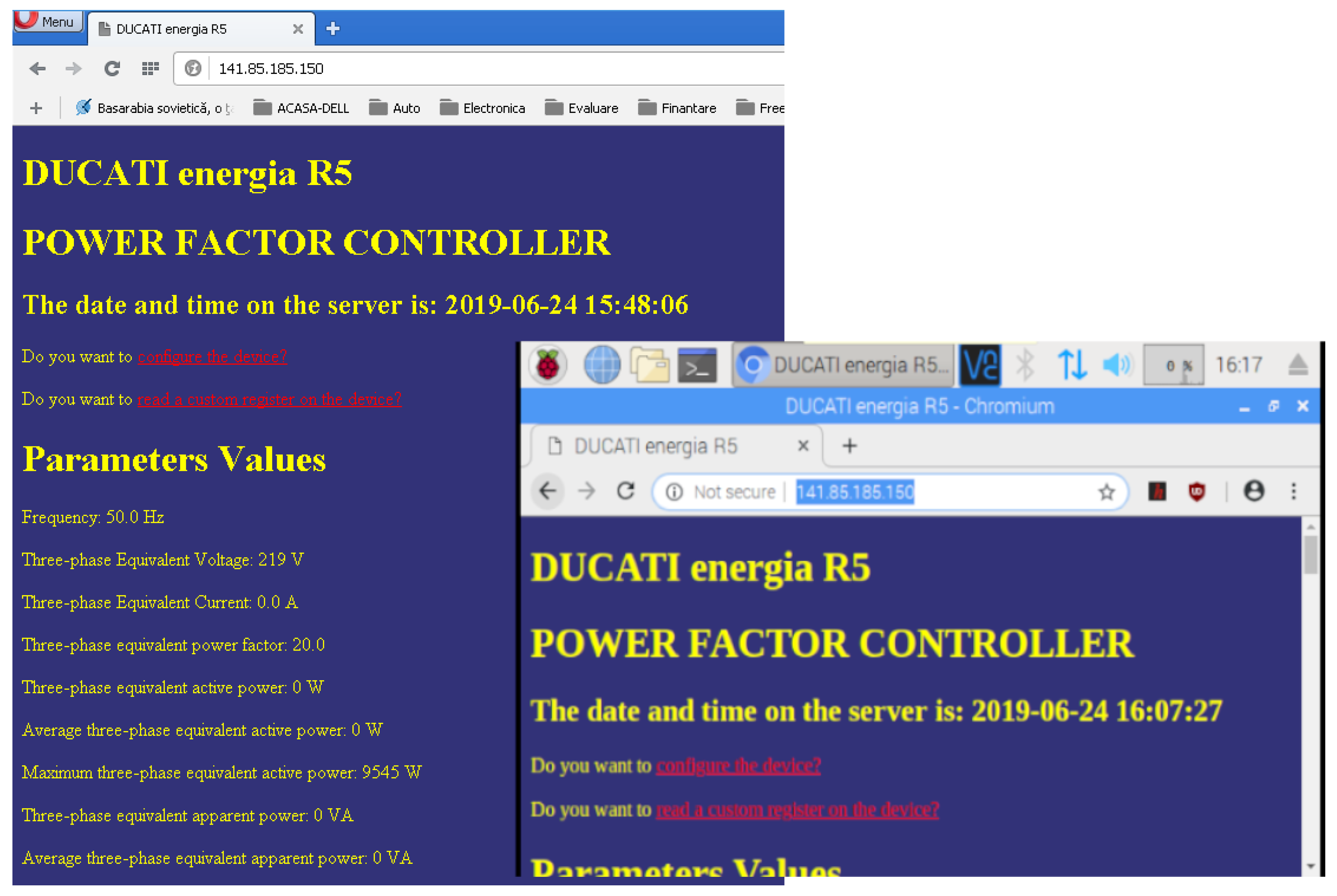
Figure 7 shows the general appearance of the application, accessed with a web browser (the captures were made from two different operating systems, Windows 10 and Raspbian, just to show the compatibility of the realized application). The data were read on the first page, and for the configuration, a more secure connection procedure was needed to avoid unauthorized configurations, which could cause damage.

4. Discussion

In order to observe the influence on the network at the connection of the capacitor battery, the voltage waveform was captured (Figure 8), where the X axis is the time representation (10 ms/div) and the Y axis the amplitude representation (1 V/div). The complexity of this measuring system was to achieve the best solution for accurate measurement. For example, choosing the best ratio of the current transformer and the best value of the secondary circuit of the current transformer resistor was necessary to achieve the best linearity and sensitivity of measurement system. Both the reduction of the current and the modification of its phase were observed after the important variation of the current from the moment of commutation, aspects that were expected to happen. The representation scale was 1 V vertically and 10 ms horizontally, per division. For the measurement, a current transformer was used, with the higher frequency band, in order not to attenuate the transient regime. For current transformers, it is mandatory to use a secondary circuit with a resistor, to prevent a faulty state in the case of open circuit. Additionally, the resistor helped convert current into voltage in order to be easily readable by the oscilloscope. The oscilloscope probes used were equipped with a 1:10 divider, in order to attenuate the measured signal. The current transformers used were manufactured by Talema India and were of the type AC1010-AC1020. For the secondary, it was provided with five turns and a load resistance of two steps, 1.8 kohms and 270 ohms (the selection was made using a jumper); see Figure 9. In this way, a higher sensitivity could be obtained from the current transformer (1.8 kohms) or better linearity (270 ohms). The observed power factor improved from 0.64 to 0.8, using a capacity of 9.6 μF and an electric motor running without load. Regarding the resistors in Figure 9, for the current transformer, it was mandatory to have a resistor in secondary circuit, because when we had an open circuit, it could be a faulty state. Additionally, this resistor converted the current into voltage to be easily readable by the oscilloscope.

During the testing of the equipment, the aim was to highlight the moment when a step connection of the capacitor batteries took place. The most convenient to use, which also provided galvanic isolation, was a broadband frequency current claw device, from DC to over one hundred kHz. The wider the frequency band, the better the transient regime was obtained. As a load, a 2.2 kW three-phase asynchronous motor was used.

The capacitors were specially designed for the correction of the power factor and contained resistors for their discharging so that at the next switching, they were not loaded with a significant voltage. This was why the equipment did not perform frequent switching, allowing no less than one minute between two switches, so that there was enough time for the capacitors to be discharged.

The interpretation of the switching moment was qualitative, highlighting the moment when it took place, and its effect on the amplitude and phase of the current. Using the PF correction device and a custom built telemetry module, we were able to adjust the configuration of the PF device remotely, as well as read and record on a server the electric current parameters. While the PF improvement was not better than other existing methods, this implementation outlined the ability to use telemetry to identify potential issues and improve the PF correction efficiency.

This power factor correction device can be a component in the emerging field of smart grids because of the remote control and measurement capabilities. It can be easily integrated in the smart grid environment using secure communication capabilities.

PF correction is very important from an economic point of view as well. In Romania, the pricing of reactive electricity to consumers, with differentiation in the case of domestic consumers, is made according to the average power factor, reported at a neutral PF, currently equal to 0.92. For a PF between 0.65 and 0.92, the pricing is done according to the energy price. If the PF is less than 0.65, the payment is calculated at three times the price of the reactive energy [35].

The estimated cost of the entire device, considering only component costs without the manufacturing process, was around 700 Euro. On the market, the price is around 165 Euro/kVA. Additionally, the cost increases when installing the power factor correction equipment (cables, settings, etc.). The comparison is valid only for the same principle of design; the cost increases considerably when another principle is used (e.g., synchronous electric drive).

For a test load of 10 kw, a benefit of 20–30% of energy efficiency was estimated. The estimation was made over five days, but to be more accurate, a longer period of time is required, e.g., several months. Due to seasons, an accurate estimation of the energy efficiency must be made over one year.

5. Conclusions

The importance of controlling and maintaining the power factor is undeniable, due to the effects that a small power factor can have on the network. There is not only an unjustified consumption, but also the possibility of the occurrence of damage, when the content of harmonics is important.

The paper presents not only a general view on the power factor and its influence on the functioning of the network, but also the dimensioning and practical realization of a proposed equipment that improves the power factor of a consumer, by connecting capacitors to the power line.

A new PFC circuit based on telemetry and remote configuration was designed and tested. The main advantage of the achieved equipment was that it could be configured and programmed remotely through an Internet connection, allowing for easy fine tuning of the algorithm’s configuration parameters to achieve potentially better operation based on the time feedback loop and artificial intelligence. This is an interesting idea that will be further explored in future work. Other advantages were related to the fact that the application was designed to ensure portability and flexibility in the operation of the equipment at various load levels depending on the targeted implementation.

The configuration possibilities of the Ducati Energia R5 device are multiple, starting with both single-phase and three-phase operation and continuing with setting parameters for the capacitors used and reaching limits for triggering alarms.

The obtained results confirmed the presented theory perfectly and showed the correctness of the equipment design. The energy losses measured on the test equipment were reduced by 20% over a short test period of five days. Accurate statistical data would require longer period tests (e.g., one year). Loss of equipment efficiency is a consequence of an improper power factor. When a plant operates with a low power factor, the amount of useful energy available inside the plant at distribution transformers is considerably reduced due to the amount of reactive energy that the transformers must carry. Less current means less losses in the distribution system of the plant, because the losses are proportional to the square of the current (I²R).

The recorded data regarding the transient regime clearly showed that the current variations could be important. In this situation, the capacities used were of a small value (μF), so the results were proportional. The influence on the obtained data was also due to the current probe. The higher the frequency band, the more spectacular the transition (by amplitude and duration).

Another interesting idea for future work can be the scheme of the measuring system for data acquisition. Simplifying the design, it consisted of conditional circuits (current transformer) and an oscilloscope. The complexity of the measuring system was focused to achieve the most accurate measurement; for example, to choose the best ratio of current transformer and the best value of secondary circuit of the current transformer resistor, which is necessary to reach the best linearity and sensitivity of the measurement system.

References

- Apetrei, D.; Chicco, G.; Neurohr, R.; Albu, M.M.; Postolache, P. Power quality monitoring. Data relevance and usefulness. In Proceedings of the 15th IEEE Mediterranean Electrotechnical Conference MELECON, Valletta, Malta, 28 Febrauary 2010; pp. 1630–1635. [Google Scholar]
- Golkar, A.; Golkar, A.M. Reactive power pricing in deregulated electricity market. In Proceedings of the 20th International Conference and Exhibition on Electricity Distribution—Part 1, Prague, Czech Republic, 8–11 June 2009. [Google Scholar]
- Li, J.; Geng, X.; Li, J. A Comparison of Electricity Generation System Sustainability among G20 Countries. Sustainability 2016, 8, 1276. [Google Scholar] [CrossRef] [Green Version]
- Bhatia, A. Power Factor in Electrical Energy Management; PDHonline Course: Fairfax, VA, USA, 2012. [Google Scholar]
- Graña-López, M.; García-Diez, A.; Filgueira-Vizoso, A.; Chouza-Gestoso, J.; Masdías-Bonome, A. Study of the Sustainability of Electrical Power Systems: Analysis of the Causes that Generate Reactive Power. Sustainability 2019, 11, 7202. [Google Scholar] [CrossRef] [Green Version]
- Emanuel, A.E. Apparent and reactive powers in three-phase systems: In search of a physical meaning and a better resolution. Eur. Trans. Electr. Power 2007, 3, 7–14. [Google Scholar] [CrossRef]
- Robbins, B.A.; Dominguez-Garcia, A.D. Optimal Reactive Power Dispatch for Voltage Regulation in Unbalanced Distribution Systems. IEEE Trans. Power Syst. 2015, 31, 2903–2913. [Google Scholar] [CrossRef]
- Pereira, B.R.; Da Costa, G.R.M.M.; Contreras, J.; Mantovani, J.R.S.; Da Costa, G.R.M. Optimal Distributed Generation and Reactive Power Allocation in Electrical Distribution Systems. IEEE Trans. Sustain. Energy 2016, 7, 975–984. [Google Scholar] [CrossRef] [Green Version]
- Kirkham, H.; Emanuel, A.; Albu, M.; Laverty, D. Resolving the reactive power question. In Proceedings of the 2019 IEEE International Instrumentation and Measurement Technology Conference (I2MTC), Auckland, New Zealand, 20–23 May 2019; pp. 1–6. [Google Scholar]
- Chang, W.-N.; Liao, C.-H. Development of an SDBC-MMCC-Based DSTATCOM for Real-Time Single-Phase Load Compensation in Three-Phase Power Distribution Systems. Energies 2019, 12, 4705. [Google Scholar] [CrossRef] [Green Version]
- Shin, H.-K.; Cho, J.-M.; Lee, E.-B. Electrical Power Characteristics and Economic Analysis of Distributed Generation System Using Renewable Energy: Applied to Iron and Steel Plants. Sustainability 2019, 11, 6199. [Google Scholar] [CrossRef] [Green Version]
- Asprou, M.; Kyriakides, E.; Albu, M. The effect of PMU measurement chain quality on line parameter calculation. In Proceedings of the 2017 IEEE International Instrumentation and Measurement Technology Conference (I2MTC), Torino, Italy, 22–25 May 2017; pp. 1–6. [Google Scholar]
- Oancea, C.-D. Power factor evaluation in data acquisition systems. In Proceedings of the 2017 9th IEEE International Conference on Intelligent Data Acquisition and Advanced Computing Systems: Technology and Applications (IDAACS), Bucharest, Romania, 21–23 September 2017; Volume 1, pp. 481–484. [Google Scholar]
- Oancea, C.D. Analysis of the performance of the mark-space method for determining the power in single-phase circuits. In Proceedings of the 2017 International Conference on Electromechanical and Power Systems (SIELMEN), Iaşi, Romania, 12–13 October 2017; pp. 448–451. [Google Scholar]
- Stoica, S.-D. The Circulation of Reactive Power and the Appearance of Resonance Phenomenon at the Final User’s Premises. In UPB Scientific Bulletin, Series C: Electrical Engineering; Politechnica University of Bucharest: Bucharest, Romania, 2011; Volume 73. [Google Scholar]
- Olaru, D.; Floricău, D. Model Analysis for Sinusoidal Power Factor Corrector. In UPB Scientific Bulletin, Series C: Electrical Engineering; Politechnica University of Bucharest: Bucharest, Romania, 2012; Volume 74, pp. 273–282. [Google Scholar]
- Fulga, N.; Popescu, M.O.; Popescu, C. On the Transients Optimization and the Power Factor Correction of the Static Converters. In UPB Scientific Bulletin, Series C: Electrical Engineering; Politechnica University of Bucharest: Bucharest, Romania, 2008; Volume 70, pp. 51–60. [Google Scholar]
- Sa’Ed, J.; Amer, M.; Bodair, A.; Baransi, A.; Favuzza, S.; Zizzo, G. A Simplified Analytical Approach for Optimal Planning of Distributed Generation in Electrical Distribution Networks. Appl. Sci. 2019, 9, 5446. [Google Scholar] [CrossRef] [Green Version]
- Charalambous, A.; Hadjidemetriou, L.; Zacharia, L.; Bintoudi, A.; Tsolakis, A.; Tzovaras, D.; Kyriakides, E. Phase Balancing and Reactive Power Support Services for Microgrids. Appl. Sci. 2019, 9, 5067. [Google Scholar] [CrossRef] [Green Version]
- Hadjidemetriou, L.; Kyriakides, E. Accurate and efficient modelling of grid tied inverters for investigating their interaction with the power grid. In Proceedings of the 2017 IEEE Manchester PowerTech, Manchester, UK, 18–22 June 2017; pp. 1–6. [Google Scholar]
- Ali, Z.; Christofides, N.; Hadjidemetriou, L.; Kyriakides, E. An advanced current controller with reduced complexity and improved performance under abnormal grid conditions. In Proceedings of the 2017 IEEE Manchester PowerTech, Manchester, UK, 18–22 June 2017; pp. 1–6. [Google Scholar]
- Sangwongwanich, A.; Yang, Y.; Sera, D.; Soltani, H.; Blaabjerg, F. Analysis and Modeling of Interharmonics From Grid-Connected Photovoltaic Systems. IEEE Trans. Power Electron. 2018, 33, 8353–8364. [Google Scholar] [CrossRef] [Green Version]
- Coman, C.M.; Florescu, A. Electric grid monitoring and control architecture for industry 4.0 systems. In Proceedings of the 2018 International Symposium on Fundamentals of Electrical Engineering (ISFEE), Bucharest, Romania, 1–3 November 2018; pp. 1–6. [Google Scholar]
- Lin, C.; Chen, M. Design and implementation of a smart home energy saving system with active loading feature identification and power management. In Proceedings of the 2017 IEEE 3rd International Future Energy Electronics Conference and ECCE Asia (IFEEC 2017—ECCE Asia), Kaohsiung, Taiwan, 3–7 June 2017; pp. 739–742. [Google Scholar]
- Tuballa, M.L.; Abundo, M.L. A review of the development of Smart Grid technologies. Renew. Sustain. Energy Rev. 2016, 59, 710–725. [Google Scholar] [CrossRef]
- Mnati, M.J.; Bossche, A.V.D.; Chisab, R.F. A Smart Voltage and Current Monitoring System for Three Phase Inverters Using an Android Smartphone Application. Sensors 2017, 17, 872. [Google Scholar] [CrossRef] [PubMed]
- Tureczek, A.M.; Nielsen, P.S. Structured Literature Review of Electricity Consumption Classification Using Smart Meter Data. Energies 2017, 10, 584. [Google Scholar] [CrossRef] [Green Version]
- Bonisławski, M.; Hołub, M.; Borkowski, T.; Kowalak, P. A Novel Telemetry System for Real Time, Ship Main Propulsion Power Measurement. Sensors 2019, 19, 4771. [Google Scholar] [CrossRef] [Green Version]
- Zhang, W.; Feng, G.; Liu, Y.-F.; Wu, B. New digital control method for power factor correction. IEEE Trans. Ind. Electron. 2006, 53, 987–990. [Google Scholar] [CrossRef]
- Jain, R.; Sharma, S.; Sreejeth, M.; Singh, M. PLC based power factor correction of 3-phase Induction Motor. In Proceedings of the 2016 IEEE 1st International Conference on Power Electronics, Intelligent Control and Energy Systems (ICPEICES), Delhi, India, 4–6 July 2017; pp. 1–5. [Google Scholar]
- Cano-Ortega, A.; Sánchez-Sutil, F.; Hernandez, J.C. Power Factor Compensation Using Teaching Learning Based Optimization and Monitoring System by Cloud Data Logger. Sensors 2019, 19, 2172. [Google Scholar] [CrossRef] [PubMed] [Green Version]
- Quick Setup Power Factor Controller (PFC) R5. Available online: https://www.ducatienergia.com/media/products/180221-1623-guida-rapida-r5-v0l-ita-eng.pdf (accessed on 1 February 2020).
- Assembly and Use Instructions R5 Power Factor Controllers. Available online: https://www.ducatienergia.com/media/products/180221-1625-mu-mid-r5-d-eng.pdf (accessed on 1 February 2020).
- Carmen Ionescu Golovanov, Measurement of Electrical Quantities in the Electric Power System; AGIR Publishing House: Bucharest, Romania, 2009.
- Electricity Pricing for Captive Consumers, SCE-POC-09-19/01.11.2002; Instructions for Charging Electricity to Captive Consumers: Bucharest, Romania, 2006.
Figure 1.
Power factor correction (PFC) device power diagram for three-phase current.
Figure 2.
Application for determining the capacity for power factor compensation.
Figure 3.
Scheme for simulating the operation of an RL circuit.
Figure 4.
Scheme for simulating the phase compensation function using a capacitor.
Figure 5.
Schematic representation of the proposed assembly for power factor correction.
Figure 6.
Capacitor battery implementation.
Figure 7.
Appearance of the main user interface (left under Windows OS, right under Raspbian OS).
Figure 8.
The appearance of the current before and after the switching moment.
Figure 9.
Current transformers used to visualize the waveform of the current at the time of switching.