Joint Emission Reduction Strategy in Green Supply Chain under Environmental Regulation


1
School of Economics, Ocean University of China, Qingdao 266100, China
2
Marine Development Studies Institute of OUC, Key Research Institute of Humanities and Social Sciences at Universities, Ministry of Education, Qingdao 266100, China
3
Faculty of Business Information, Shanghai Business School, Shanghai 201400, China
*
Author to whom correspondence should be addressed.
Sustainability 2020, 12(8), 3440; https://doi.org/10.3390/su12083440
Submission received: 27 February 2020
/
Revised: 14 April 2020
/
Accepted: 14 April 2020
/
Published: 23 April 2020
(This article belongs to the Section Economic and Business Aspects of Sustainability)
Abstract
:Under the threat of global warming, joint emission reduction strategy has been widely adopted as an effective solution for the industry to guarantee environmental sustainability. In the practice of supply chain, environmental regulations and supply chain contracts are applied with the attempt to improve environmental performance. However, whether these measures are actually effective remains unanswered. In this paper, we study a supply chain with one manufacturer and one retailer adopting joint emission reduction strategy. We first investigate under what circumstance the environmental regulation can effectively result in higher emission reduction efforts. The result shows that when the cost coefficient satisfies certain conditions, the increase of penalty or subsidy can lead to more investment in emission reduction. In addition, if the environmental impact caused by the production process is extremely high, the enforcement of the regulation is ineffective. We also explore how the cost-revenue-sharing contract affects the emission reduction strategy and the coordination of the members in the supply chain. The results suggest that the incentive effect of environmental regulation is more effective when the supply chain coordination contract exists. Numerical experiments are also presented to verify our analytical conclusions.
1. Introduction
Since global warming became a significant threat to human beings, emission reduction has obtained great attention from governments, industries, and consumers all over the world. Facing the exacerbating climate change, effective measures that can reduce carbon emissions are more crucial than ever for the government. In 1992, for the common purpose of maintaining a stable greenhouse gas level, the United Nations formulated the United Nations Framework Convention on Climate Change. Since the Kyoto Protocol in 1997, many environmental regulations such as the cap-and-trade scheme and the carbon tax policy, have been verified to be effective measures to reduce carbon emissions in the USA and Australia [1]. In India, the government is planning to electrify most of the new vehicles by 2030, which forces traditional gasoline automobile manufacturers to redesign their products. Other national strategies such as “German industry 4.0” and “Made in China 2025” also show unprecedented determination for the development of green manufacturing [2].
In a matter of fact, the environmental impact caused by industrial activities is difficult to be completely avoided [3]. Therefore, both the governments and the enterprises are actively looking for new industrial frameworks to reduce greenhouse gas emissions more effectively. For instance, the central government in China adopted a sales subsidy policy by offering subsidies up to RMB 30,000 for each plug-in hybrid electric vehicle and up to RMB 55,000 for each battery electric vehicle [4]. In another example, in the U.S., the government had enacted the “Corporate Average Fuel Economy (CAFE)” regulations which stated that “if the average mpg (miles per gallon) of a manufacturer’s annual fleet production falls below the specified standard, the manufacturer must pay a penalty” [5]. The government also advertises for the manufacturers who meet the defined standards on its official website which grants a verified ‘green image’ to them. This ‘green image’ adds extra brand value to their environment-friendly vehicles. Thus, the regulation creates a competitive edge for these automobile manufacturers who comply with it and effectively stimulates the manufacturers to actively invest in the emission reduction effort in their production process.
Meanwhile, an increasing number of consumers have shown their preference for low-carbon, no-pollution, and energy-saving products. Research by Accenture demonstrates that more than 80% of the interviewees consider the green level (i.e., the more efforts to reduce emissions, the higher the green level) of the product when making purchasing decisions, and they are also willing to pay a higher price for the green products with lower emission [6]. Given this feature of the consumer market, the joint emission reduction strategy has been widely adopted as an effective solution for enterprises to guarantee environmental sustainability [7]. It consists of the manufacturer’s emission reduction effort in the productive process and the retailer’s advertising effort in the marketing process, aiming to improve the performance of the supply chain. For example, during recent years, the automakers, such as General Motors and Ford Motors, have focused more on designing new energy vehicles to reduce the carbon emission. Additionally, taking Walmart as another example, it outlined an advertising strategy for promoting its cooperative partners’ green products, through which both the manufacturers and Walmart can gain economic benefits as well as fulfilling the environmental responsibility by selling more green products simultaneously [8].
With the concern of social responsibility, environmental regulations and consumers’ green preference, the players in the supply chain are facing a more complex and uncertain market environment. It is worth noting that, as a part of the supply chain, the effect of emission reduction by firms individually is limited [9]. Self-interested emission reduction action without coordination with other firms is difficult to minimize the carbon emissions of the supply chain. To avoid such selfish behavior, maintaining strategic partnerships is an advantageous option for both the manufacturer and the retailer [10]. Hence, the introduction of appropriate coordination mechanisms can play a positive role in improving overall performance. What is more, we are also eager to know whether the introduction of the coordination mechanism under environmental regulation is effective in reducing carbon emissions.
In this paper, we mainly explore and answer the following questions:
- (1)
- How do the players in the supply chain make pricing decisions, green level decisions and advertising decisions concerning supply chain structure, environmental regulation, and supply chain contract?
- (2)
- How does the environmental regulation impact the green level of the product and the advertising effort?
- (3)
- Can the environmental regulation and the cost-revenue-sharing contract effectively improve the performance of the joint emission strategy?
To answer the questions above, a Stackelberg game model is developed to investigate the decision of the members in a two-echelon supply chain. The manufacturer invests in the production process and produces a green product to satisfy the demand of the environmental conscious consumer. The retailer pays the advertising effort for green-marketing, such as cultivating a green consumption concept by environmental advertisements or releasing the information of the green product. The joint emission reduction strategy is determined by the members in the supply chain jointly to maximize their profit. To investigate the effect of environmental regulation on joint emission strategy, we compare the decisions of members in the decentralized and centralized supply chain models with and without the regulation. We also design an effective coordination mechanism and investigate whether it can achieve Pareto improvement in the decentralized model. Besides, we explore how to balance social welfare and corporate profits by modeling analysis under environmental regulation. The work above provides managerial insights for the formulation of environmental regulations.
The remainder of this paper is organized as follows. Section 2 provides a brief literature review and Section 3 introduces the notations and proposes the basic model. Section 4 derives the theoretical results of centralized, decentralized models and the social welfare maximum model. The cost-revenue-sharing contract is analyzed under environmental regulation in Section 5. Conclusions are drawn in Section 6.
2. Literature Review
The literature related to our study covers three streams of research: sustainable supply chain management, environmental regulation, and supply chain coordination.
2.1. Sustainable Supply Chain Management
With the development of a low-carbon economy, sustainable supply chain management has become a hot issue in the academic community. Drumwright [11] pointed out that enterprises should have a sense of social responsibility and focus on social benefits while pursuing economic benefits. Within the theme of low-carbon economy, several scholars have been concerned about the problems of green product design, remanufacturing, green procurement system and reverse logistics [12,13,14,15,16]. Ji et al. [17] focused on the sales channel selection for the manufacturers and found that when the degree of consumers’ green preference exceeds a certain value, the introduction of the online channel is more profitable. In terms of consumer purchasing behaviors, Hong et al. [18] compared the optimal pricing strategies of green products under different scenarios and summarized that the pricing strategies are better off for the firm. Taking into account environmental performance, Raitasuo et al. [19] investigated the relationship between green supply chain management skills and environmental performance in different countries. Narimissa et al. [20] analyzed drivers and barriers for implementation and improvement of sustainable supply chain management, aiming to create and improve sustainability in the Iranian oil and gas supply chain. For more related works of literature, readers can refer to Brandenburg et al. [21], Golicic and Smith [22], Wolf [23], Beske et al. [24], Saberi et al. [25], Zimon et al. [26], Koberg and Longoni [27].
2.2. Environmental Regulation
Facing the challenge caused by environmental pollution, some researchers tried to study the manufacturer’s production and pricing strategy under the interference of the government [28,29,30]. Chen [31] pointed out that strict environmental regulations may be non-effective for environmental improvements. Krass et al. [32] discussed the influence of environmental taxes on manufacturers’ choice of emissions-reducing technologies. Moner-Colonques and Rubio [33] evaluated the effect of emission tax and emission standards and analyzed the impact of the monopolist’s strategic behavior. The results showed that adopting emission tax is the optimal policy since it yields higher welfare than a non-committed regulation. Considering Extended Producer Responsibility (EPR) legislation, Subramanian et al. [34] studied the impact of EPR policy on product design and supply chain coordination. In terms of composite regulations, Gouda et al. [35] investigated the product design strategy of automakers. Martín-Herrán and Rubio [36] characterized the optimal environmental tax policy to regulate a polluting monopoly when the enterprise can invest in abatement technology. Cohen, Cui and Gao [4] investigated the effect of government support on green product design and environmental impact. The results showed that sales subsidy is more effective in promoting the development of green technologies rather than direct R&D. Concerning environmental regulation, Ghosh, Shah and Swami [5] solved the optimal production decisions of two competing manufacturers and pointed out that it would be more significant to compare the results under a sequential game.
Some literature also studied the production and pricing decisions of participants in the supply chain under environmental regulation [37,38]. Chen and Sheu [39] investigated a rational environmental regulation mechanism that could promote EPR for the participants in the green supply chain. Fahimnia et al. [40] proposed a supply chain model integrating economic and environmental objectives. Similar to our study, some scholars studied the emission reduction strategy of firms under environmental regulations. Assuming that demands were influenced by the product’s emission reduction of the manufacturer and the retailer’s promotion in marketing, Xu et al. [41] established three differential game models to compare the optimal decisions. In the dual-channel supply chain, Zhou and Ye [7] structured a differential game model to explore the joint emission reduction strategies and designed the cooperative advertising contract. Wang et al. [42] explored the significant effect of the cap-and-trade mechanism on the manufacturer’s production decisions and carbon emissions. Considering emission reduction and remanufacturing, Xu and Wang [43] analyzed the optimal decision strategy and profit distribution of a closed-loop supply chain (CLSC) with emission reduction dependent demand.
In this paper, assuming that the consumers have low-carbon preference, we investigate the effect of environmental regulation on joint emission reduction strategies and contract design decisions in a two-echelon supply chain.
2.3. Supply Chain Coordination
The coordination mechanism can be used to coordinate the corporations in the decentralized supply chain to achieve performance improvement for the overall supply chain. Taking into account economic, environmental, or social goals, a variety of contracts have been proposed for guiding the cooperation in the supply chain [34,44,45]. Hong and Guo [8] compared the environmental performance resulting from the green-marketing cost-sharing contract and two-part tariff contract. Song and Gao [46] quantitatively analyzed the impact of the revenue-sharing contract on the internal membership decision variables and designed a new contract that can effectively improve the overall profit of the supply chain. Considering channel disruption, Aslani and Heydari [47] proposed a transshipment contract to coordinate the enterprises in the supply chain which guarantees the profitability of each player. Xue et al. [48] explored the value of a buyback contract by analyzing a model which includes one manufacturer and two competing retailers. The results showed that the asymmetric contract structure is better off for the whole supply chain. Chauhan and Singh [49] summarized the model-based research on coordination mechanisms in sustainable supply chains and provided an in-depth analysis of the widely-used models. In terms of the cap-and-trade mechanism, Cao and Yu [50] constructed three different contracts to investigate the operational decision of one manufacturer and one capital-constrained retailer in an emission-dependent supply chain. The results showed that a revenue-sharing contract can achieve Pareto improvement of the total profit under certain conditions. Based on the literature above, we investigate the effect of environmental regulation on joint emission reduction strategy under several contracts, and whether the regulation can achieve Pareto improvement for the overall performance.
In conclusion, environmental concerns have received significant attention from scholars. However, to our best knowledge, only limited studies have explored the influence of environmental regulation and joint emission reduction strategy on decisions of the supply chain simultaneously. In contract to the above research, the contributions of this paper are as follows. Firstly, we consider the consumer’s green preference, joint emission reduction strategy and environmental regulations in the supply chain. Secondly, we obtain the optimal decisions of the manufacturer and the retailer, as well as analyzing the impact of changes concerning the correlation coefficient on the profit of the supply chain. Thirdly, we investigate the role of environmental regulation from the perspective of maximizing social welfare. Lastly, the coordinating mechanism is designed to achieve the Pareto improvement in the decentralized supply chain. In order to solve the above, a Stackelberg game model is structured, where the manufacturer invests in emission reduction during production and the retailer invests in green-marketing. Moreover, we analyze the impact of environmental regulation on the optimal decisions and verify the effectiveness of the environmental regulation on restricting participants’ behaviors under contract. By numerical analysis, we summarize some managerial insights which are useful for enterprises to improve the profit and environmental responsibility, as well as for governments to make policy.
3. Problem Notations and Assumptions
With consideration of the consumers’ green preference, this paper investigates the impact of government regulation on the emission reduction strategies of supply chain members. Compared to the traditional product, the price of the green product is usually higher because they provide the higher value for the consumer. When the traditional and the green products are sold simultaneously in the market, the phenomenon of “bad money drives out good” may occur [51]. To avoid this, the retailer can adopt a green-marketing strategy to stimulate environmentally-conscious consumers to purchase green products. Therefore, we construct a model that consists of a manufacturer and a retailer, where the manufacturer determines the wholesale price and the emission reduction effort, and the retailer determines the selling price and the advertising effort.
For simplicity but without loss of generality, some main assumptions are defined as follows.
Assumption 1.
The fixed cost of production for the manufacture is, the wholesale price of the product is, the unit selling price of the product is, and.
Assumption 2.
Erickson [52] and Zhang et al. [53] presented that market demand is a linear expression of price and non-price factors. In this paper, the demand is a linear function of selling price, the green level of product, and the advertising effort, i.e.,
wheredenotes the potential demand of the product in the overall market,denotes the elastic coefficient of customer demand with respect to the price. Previous studies have proved that green level of the product and the advertising effort positively affect the consumer demand [54,55]. Additionally, the authors of [41] assume that the green level of product and the advising effort of the retailer are measurable and quantifiable. In addition, Xue et al. [56], Han and Wang [57], Wu [58], Xing et al. [59] introduce similar variables to represent firms’ emission reduction efforts in their researches. A largerepresents a higher green level; the higher the green level, the more investment in emission reduction during the production. Similarly, a largerepresents the more advertising efforts; the more advertising efforts, the more investment in green-marketing during the selling period. Besides,anddenote consumer’s demand sensitivity concerning the green level and the advertising effort. Assume that when the manufacturer can get rid of all emission during the production process, the corresponding green level is defined as. However, in the reality, due to the undeveloped environmental technology, it would be extremely expensive to maintain a high green level for the manufacturer, and no company can raise the green level towhen still being profitable. Thus, we assume thatandare sufficiently high and always holds in our study.
Assumption 3.
Considering the investment of the members in the production, letdenote the investment of the manufacture for the emission reduction. Assume thatis a non-negative convex non-decreasing function of the green level, and it should satisfy the conditions,,. Convexity of costs can be attributed to diseconomies of scale where investment is involved. To explain further, it is easy to obtain the ‘low hanging fruit’ for firms during greening while subsequent greening improvements will be incrementally more difficult. Without loss of generality, we setto express the diminishing marginal return of the green level concerning the investment, wheredenotes the cost coefficient of the green level [1,9,56,60,61]. Similarly, the green-marketing investment of the retailer is noted as a non-decreasing convex function of the advertising effort, i.e.,, whererepresents the cost coefficient of advertising effort [41].
Assumption 4.
We consider both government penalty and subsidy in our model based on the observation of Corporate Average Fuel Economy (CAFE) regulation. According to this regulation, every automobile retailer has to reach a minimum sales-weighted average fuel efficiency (i.e., 27.5 Miles per Gallon) in the U.S. [62]. Retailers who fail to meet the specified standard incurred a penalty of $5 per car per 1/10 of a gallon. Hence, we assume that the government sets the standard for the green level. Letdenote the penalty or subsidy per unit deviation from the defined green standards for every single product. Given the assumption, the government can levy a penalty for every unit green level that the firm falls short of, i.e.,, given by[4,5]. Nevertheless, the expression of penalty ensures that, in the case where the green level of the products is higher than the regulation standard, a subsidy is awarded to the firm ().
Moreover, the notations used in this paper are presented in Table 1. The implications of the endogenous and exogenous variables involved in the model have been explained in the above assumptions.
4. Model Solutions and Discussions
We use subscripts to represent the manufacturer, the retailer, and the supply chain, respectively. Under the joint emission reduction strategy, the manufacturer invests in emission reduction during the production process, while the retailer makes an effort to advertise the green product for attracting more consumers with green preferences [7]. With the goal of exploring the optimal strategies of the manufacturer and the retailer, as well as the impact of the regulation under different scenarios, we construct the following models: centralized and decentralized supply chain models with/without environmental regulation, and decentralized supply chain model under social welfare maximizing criteria.
4.1. Centralized Decision Model
4.1.1. Without Environmental Regulation
In the centralized supply chain (denoted by superscript ), there exists a central planner who jointly arranges the decisions on the green level, price and the advertising effort for the manufacturer and the retailer so as to optimize the total profit of the supply chain. The objective function can be written as follows:
The reverse-solution method for the Stackelberg game is used to solve the problem. The same method can be referred to as Ghosh et al. [5], Tao [9], Xue et al. [56], Dong et al. [63] and Liu and Nishi [64]. Accordingly, we can obtain the following conclusions.
Proposition 1.
When the conditionis satisfied, the Hessian matrix for the supply chain profitconcerningis negative definite. The objective function has a maximum value, and optimal equilibrium solutions are as follows:
For , the bound on maintains the non-negativity of the optimal equilibrium solutions [1,56,65]. It can be seen that the objective function is a joint concave function of , and the target function has a maximum. The reason we only consider the case when is that, if holds, the optimal solution of at least one of the variables among , , would reach the upper bound (or infinite), then our problem would be meaningless and unrealistic.
Proposition 1 shows that a higher green preference (i.e., a large ) of a consumer stimulates the manufacturer to raise the green level and stimulates the retailers to invest more on green-marketing. Moreover, the cost coefficient of emission reduction and the cost coefficient of advertising effort have a negative impact on the green level.
4.1.2. With Environmental Regulation
In this section, we consider a penalty factor to represent the penalty or subsidy per unit deviation from the green standard of a single product (denoted by subscript and superscript ). If , represents the penalty cost charged by the government; otherwise, represents the unit subsidy awarded to the manufacturer [4,5]. Then the objective function can be written as follows:
Proposition 2.
Under environmental regulation, the optimal green level of product for manufacture is as follows:
For , the bound guarantees the non-negativity of the optimal equilibrium solutions. Proposition 2 shows that when the cost coefficient of emission reduction is higher than , the manufacturer falls short of the standards mandated by the government. Clearly, it becomes difficult for the manufacturer to increase the investment in emission reduction during the production process. However, if , the manufacturer prefers to step up efforts to reduce carbon emissions and obtain the government subsidy. We illustrate the relationship between the cost coefficient of emission reduction and the optimal green level in Figure 1. As shown in Figure 1, with the increase in the cost of emission reduction , it is profitless to invest more in reducing carbon emissions for the manufacturer .
Further, under the environmental regulation, we use the same reverse-solution method to obtain the optimal equilibrium solutions as follows:
Corollary 1.
In the centralized model, the effect of the environmental regulation on the equilibrium strategies are presented as follows:
- (1)
- The optimal green level of product increase in if ;
- (2)
- The optimal advertising effort of retailer decrease in if ; where
Corollary 1 indicates that the joint emission reduction strategy varies as changes. We illustrate this further through Figure 2, which shows that the green level of the product increases with the penalty (or subsidy) . That implies that the enforcement of environmental regulation can effectively incentivize the manufacturer to reduce emissions with more efforts. However, under a higher value , the retailer is negative in green-marketing, i.e., lower advertising effort. This conclusion also has practical economic significance. For example, a product with higher green level attracts higher customer demand, and the retailer can make more profits without increasing advertising costs.
Corollary 2.
Optimal price, advertising effortand the profitdecrease in; optimal advertising effort, green level of productand the profitincrease in.
Corollary 2 demonstrates the effect of the cost coefficient of emission reduction I and consumers’ demand sensitivity of green level on the retailer’s optimal decisions. As shown in Figure 3, with the increase in , the retailer maintains their margins by increasing price. Lower green levels and the higher price will decrease buying appetites of consumers in the future. This further leads to a decline in the profitability of the supply chain. However, the increase of consumers’ green preferences can offset the negative effect of the emission reduction cost. Therefore, the firms can benefit from improving the awareness of environmental protection and guide the consumers to see more value in green consumption. There are a series of measures to help firms for the government. For example, in America, the environmental protection department can punish the manufacturers who fall short of the mandated standard and announce the actual carbon footprint of the product to the consumers, for attracting consumers’ attention to the green product [5]. Even in emerging economies like India, the government has required firms to rethink the existing product designs aiming to electrify all new vehicles by 2030.
4.2. Decentralized Decision Model
In the decentralized supply chain (denoted by superscript ), the manufacturer and the retailer are independent self-interested entities that aim to maximize their profits. As the leader of the supply chain, the manufacturer first makes decisions on the green level of product and the wholesale price ; then the retailer determines the advertising effort and price . This sequential decision problem forms a Stackelberg game between the manufacturer and the retailer.
4.2.1. Without Environmental Regulation
We first consider the situation where the government does not impose environmental regulation in the green product market. Consequently, the profit of the manufacturer and the retailer can be written as
By applying backward induction, we derive the equilibrium solution where the manufacturer and the retailer optimize their profit in the following proposition:
Proposition 3.
In the decentralized supply chain, if the environmental regulation is not implemented, the optimal equilibrium solutions for the Stackelberg game and the results of profit are given by:
4.2.2. With Environmental Regulation
In this section (denoted by superscript and superscript ), we explore the role of environmental regulation through a comparative analysis between the scenario with and without the environmental regulation. Additionally, we discuss how to balance social welfare and corporate profits by modeling analysis from the side of the government [56].
The objective functions of the manufacturer and retailer can be written as:
Proposition 4.
In the decentralized supply chain, if the environmental regulation is implemented, the equilibrium solutions of the Stackelberg game and the results of profit are given by:
Next, we compare each member’s decision in the equilibrium under the scenarios with or without environmental regulation.
Corollary 3.
In the decentralized supply chain, the optimal joint emission strategy with and without the regulation has the following properties:
- (1)
- ;
- (2)
- , where ;
- (3)
- , where .
From Corollary 3(1), it can be referred that environmental regulation plays an effective role in inducing the manufacturer to invest more in emission reduction; while social responsibility and consumers’ green preference may also encourage the manufacturer to reduce carbon emissions. In fact, some environmental measures of the firms are indeed proposed after the government imposes environmental regulation. For example, in Europe, OEMs (Original Equipment Manufacturer) like Volvo, are committed to improving the manufacturing technique to reduce the impact on the environment [5].
We further demonstrate Corollary 3(2) by Figure 4b, which shows the impact of environmental regulation on the retailer’s advertising effort. Under a lower value of , the retailer will provide a lower advertising effort than . On the contrary, it is beneficial to invest more in advertising strategy. Additionally, higher advertising efforts can further encourage the manufacturer to provide a higher green level of product in turn and create a virtuous cycle for the emission reduction strategy. Consequently, the whole system may benefit from environmental regulation.
The pricing strategy of the retailer varies as changes in Corollary 3(3). If the value of is lower than , the retailer is inclined to adopt a “lower price” strategy, i.e., charging a lower price than the case without regulation. Conversely, the retailer prefers to raise the price as the penalty (or subsidy) increases. We further illustrate the result through numerical analysis (refer to Figure 4). Under a lower value of , the manufacturer provides a lower green level than the regulation standard and pays the punishment (refer to Figure 2). As a follower, the retailer can only decrease the price to attract consumers with lower green preferences. With the increase of , the pressure from the government will encourage the manufacturer to provide a higher green level with more efforts, which increases the consumers’ purchasing willingness. Thus, adopting a “higher price” strategy to obtain higher marginal returns is beneficial for the retailer. The analysis above indicates that the emission reduction and pricing strategy vary with the change of . Despite that the environmental regulation is imposed on the manufacturer, it still influences the decision of the retailer.
Corollary 4.
The total profit of the supply chain in the four cases (under the centralized model without/with environmental regulation, under the decentralized model without/with environmental regulation, respectively) have the following properties:
- (1)
- For , then ;
- (2)
- There are that make the following corollary true. for , for , for and for , where is constrained to in which , , , and, .
Corollary 4(1) indicates that under the centralized model, the overall profit is always higher than the case under the decentralized model, which is caused by the “double marginal effect”. In general, the well-known “double marginal effect” refers to when there is a single upstream seller (such as the manufacturer) or a single downstream buyer (such as the retailer) in the market; the upstream and downstream enterprises experience two markups (marginalization) on the whole supply chain to maximize their respective interests [66,67]. In fact, the decision-making behavior between upstream and downstream enterprises, which only considers their interests in terms of the product price and quality promotion technology, is a form of double marginalization. The phenomenon means the profit of the whole supply chain is inevitably damaged and is the result of uncooperative supply chain members.
Corollary 4(2) highlights the role of environmental regulation under different scenarios. Figure 5a,c demonstrate the impact of on the profit of the manufacturer, the retailer and the supply chain, respectively. When , with a lower green level () and selling price (refer to Corollary 3), the overall profit is undoubtedly lower than the case without environmental regulation. Otherwise, the optimal green level of the product is higher than , the manufacturer obtains the subsidy, and the overall profit is also higher than .
Figure 5b,d demonstrate the following two conclusions. Firstly, the increasing cost of emission reduction decreases the profit of the two members and the supply chain. Secondly, environmental regulation can partially offset the negative effect caused by the cost of emission reduction on supply chain members’ profit. That is to say, when the government implements environmental regulation, supply chain members become less sensitive to the cost of emission reduction.
The above conclusions have demonstrated the effect of environmental regulations on emission reduction strategy; then we will conduct modeling analysis from the perspective of consumer surplus and social welfare. In the previous literature, some researchers have studied relevant environmental policies from different aspects [28,29,30,32,33]. The next section intends to answer two questions:
- (1)
- Whether the manufacturer and retailer can provide socially optimal green efforts under environmental regulation?
- (2)
- If not, under what condition are the manufacturer and the retailer willing to provide socially optimal green efforts?
To solve this problem, we first define the value of consumer surplus (abbreviated to CS) in the following equation. The calculation process is given in the Appendix A.
In Equation (11), denotes the inverse demand function, denotes the demand of the product, denotes the demand function.
Corollary 5.
The Consumer surplus decreases with the emission reduction coefficient and the advertising cost coefficient increases with the consumers’ green preference coefficient .
Corollary 5 shows that high emission reduction cost is still the main challenge in reducing carbon emissions for the supply chain. However, consumers with higher green preferences can offset the negative effect of this. Accordingly, the government can play a dual role. Firstly, it is beneficial to create the green market by raising awareness of consumers towards green products. Secondly, in the environmentally-conscious market, penalty or subsidy policy can be used to influence the decisions of players in the supply chain. Based on consumer surplus, we further calculate the optimal value of social surplus (denoted by SS) in the following equation.
In Equation (12), and denote the profit of the manufacturer and the retailer under the decentralized model, respectively, and denotes the government revenue or expenditure which equals to [56]. When calculating the social surplus, the environmental impact (noted as ), which refers to the degree of environmental pollution during production, should also be taken into account. For the sake of measuring this effect, we assume can be given by [5]. E is the environmental impact factor, which represents the environmental impact caused by per unit deviation of green level from the regulatory standard for producing a single product. A large represents that there is more carbon emission in the production of the product. Similarly to the government penalty (or subsidy), if , denotes the negative impact of products on the environment. Conversely, can be thought of as the positive impact on the environment caused by qualified green products.
To answer the first question in this section, we solve the equilibrium solution by maximizing social welfare. The calculation process can refer to the Appendix A.
Corollary 6.
For , , , , , if , ; if , .
When the value of equals (environmental impact factor), it can be inferred that . Therefore, the socially desirable values are greater than the equilibrium solution under the decentralized supply chain . In other words, concerning emission reduction cost and environmental regulation, the manufacturer and the retailer are unable to invest in emission reduction as much as socially desirable outcomes. Accordingly, the green level and the advertising effort of products provided by the supply chain are lower than the socially desirable outcomes. For consumers with green preference, the demands of green products are also below the socially desirable outcomes. In terms of the retailer’s pricing strategy, when the cost coefficient emission reduction is relatively low, the equilibrium price will be lower than the socially optimal under decentralized model; otherwise, the retailer will charge a higher price to obtain more profit margin.
Proposition 5.
When there are more carbon emissions in the production of the product ( is large), the implementation of environmental regulation cannot incentivize firms to provide socially desirable outcomes.
The result in Proposition 5 shows that the incentive effect of environmental regulations on firms is limited under certain circumstances. When the regulation induces firms to make more efforts to reduce emissions, it does not drive firms to provide socially optimal outcomes. We illustrate the result of Proposition 5 through numerical analysis. Figure 6 shows that, for the manufacturer, if the environmental damage caused by the production is relatively small (e.g., ), the government can raise the penalty or subsidy to increase a manufacturer’s emission reduction effort as the society expects (e.g., K = 5.2, ). Otherwise, government regulation is not able to increase social welfare. Additionally, no matter how changes, the retailer is always unable to provide socially desirable outcomes.
The result in the numerical analysis above is in accordance with the practice. When the product affects the environment severely during the production process, the environmental regulation cannot induce the members in the supply chain to provide the socially optimal outcomes. Thus, for policy-makers, it may be effective to encourage the adoption of green technologies, stimulate research and development programs, and support the technology cooperation to design and develop green products.
5. Emission Reduction Cost-Revenue-Sharing Contract
In this section, we design a cost-revenue-sharing contract with the goal of exploring the effect of the contract. The coordination mechanism can be summarized as follows (denoted by superscript ): The manufacturer and retailer enter this contract to maximize their profit. The retailer shares the partial cost of emission reduction with the manufacturer, and obtains a share of the government subsidy from the manufacturer, which is the proportion of the share. The implementation of the contract needs to satisfy two constraints, . That is, both the profit of the manufacturer and the retailer can be improved.
Accordingly, the profit functions of the manufacturer and retailer are:
Similar to the decentralized problem without a contract, this problem is also a Stackelberg game, so we also solve this problem following backward induction. The solutions are given by:
Corollary 7.
(1) , ;
(2) When , ; when , the retailer’s profit is optimized; when , ; when , the overall profit of the supply chain is optimized.
According to Corollary 7, we can obtain two conclusions. As shown in Figure 7, firstly, under the decentralized model, the contract stimulates the manufacturer and the retailer to increase investment in emission reduction and green-marketing. Second, when , as increases, the retailer tends to share more emission reduction costs of the manufacturer to maximize their interests (), and the overall profit of the supply chain increases. When , with the increase of , the profit increase of the manufacturer is larger than the profit decrease of the retailer. Thus, the overall profit of the supply chain still increases. Consequently, the contract can achieve Pareto improvement for the supply chain. However, for the retailer, it needs to pay more for emission reduction, but cannot get the same amount of sales. As a result, the retailer will not set the share proportion to .
Compared to the decentralized model without a contract, the manufacturer gets more profit with the cost-sharing contract. Hence, the manufacturer must compensate the retailer in some way, and negotiate with the retailer to improve the share of the investment from to
Proposition 6.
A “win-win” situation in the decentralized model under the cost-revenue-sharing contract can be achieved for both the manufacturer and the retailer if .
According to the “win-win” strategy, the cost-revenue-sharing contract should be effective when the profit of both members is greater than that under the decentralized model, that is, . Then we can calculate the share of investment as follows: .
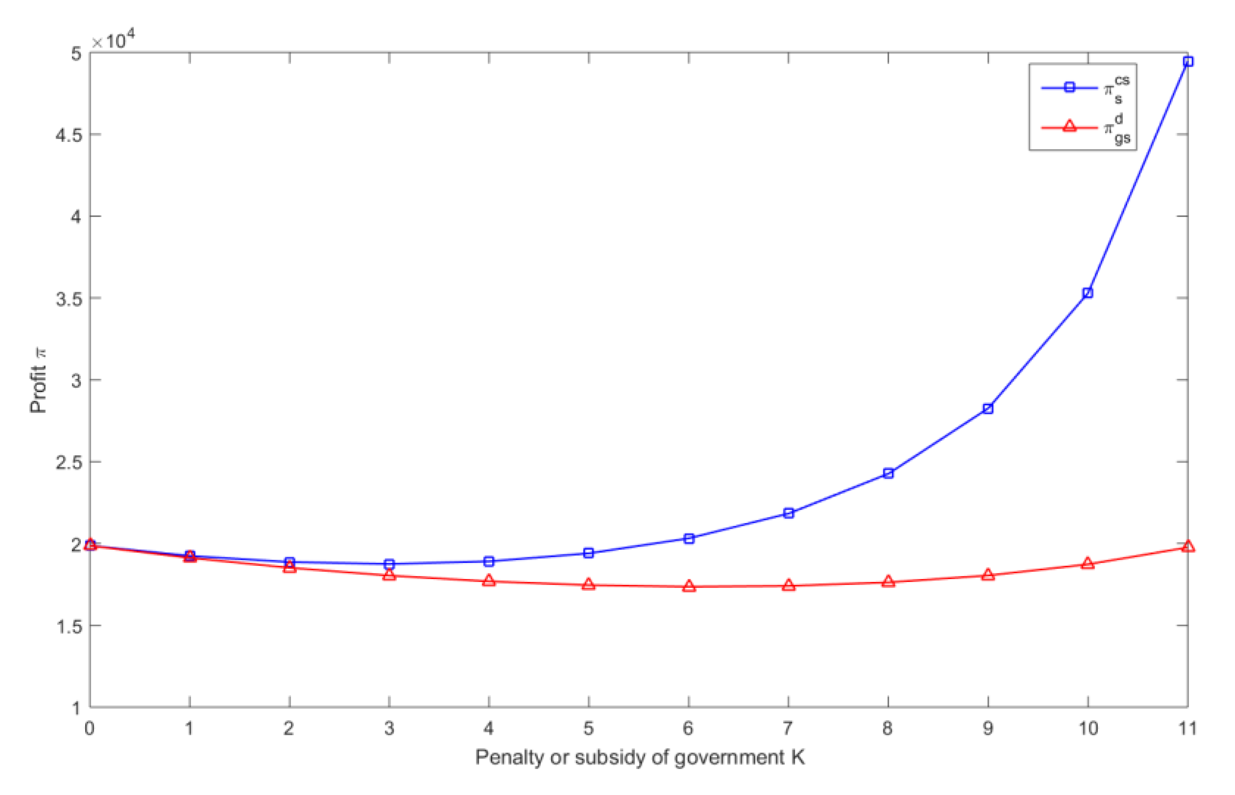
To further demonstrate the validity of the contract, we use Figure 8 to present the relationship between the penalty and the overall profit. Under the decentralized model, the growth of is higher than with the raising penalty . That is, the incentive effect of the environmental regulation with the contract is better than that without the contract. For the government, except for prompting a larger green market, taking measures to encourage coordination of the firms is also necessary, which could further improve the effectiveness of the environmental regulation.
6. Conclusions and Future Research
Under the threat of the global warming problem, choosing the optimal joint emission reduction strategy and coordination mechanisms are of great practical significance for both the manufacturer and the retailer. In this article, we propose a game model between a retailer and a manufacturer under pressures of the rising greening costs and environmental regulation. We also investigate the impact of environmental regulation on operational decisions in a decentralized and centralized model. We conclude that under certain conditions, the implementation of environmental regulation can instruct the manufacturer and the retailer to invest more in carbon emission reduction. Besides, with the increase of the government’s penalty, the manufacturer would raise the wholesale price to reduce the profit loss caused by regulation, while the retailer would raise the price to protect their interests. Ultimately, the higher price of the product would reduce the consumers’ surplus.
A higher emission reduction cost is another challenge in reducing emissions for firms in the supply chain. Due to the high emission reduction cost, the optimal green level determined by the manufacturer is lower than that under the social target, while the price determined by the retailers is higher than that under social target. Besides, if the environmental damage of the product is large enough, the enforcement of regulation is not effective to make manufacturers provide a higher green level. Finally, we observe that the implementation of environmental regulation is more effective under the cost-revenue-sharing contract. In addition, encouraging the development and application of green technologies, helping firms lower the emission reduction cost, improving the environmental awareness of consumers, and advocating greater cooperation between supply chain members, are also important aspects for the consideration of policy-makers.
This paper serves as an initial step for future work in exploring the effect of environmental regulations in the green supply chain. The current work is limited by the assumption of deterministic demand functions. Future research could investigate current problems under stochastic demand functions and green effort. It is also an interesting direction to extend the work to multiple suppliers and retailers. We have studied the vertical competition in a supply chain in this paper, while there also exists horizontal competition between supply chains in the market. Additionally, the impact of information asymmetry on the selection of emission reduction strategies between competing manufacturers could lead to additional management insights for practitioners.
Author Contributions
Conceptualization, W.Z.; methodology, formal analysis, W.Z. and J.X.; software, validation, writing—original draft preparation: J.X. and L.C.; writing—reviewing and editing, L.C. and W.Z. All authors have read and agreed to the published version of the manuscript.
Funding
This research was funded by the MOE (Ministry of Education in China) Project of Humanities and Social Sciences [18YJCZH247]; Shandong Social Science Planning Funds [18DGLJ01]; China Postdoctoral Science Foundation [2017M622287] and National Social Science Foundation [18VSJ067].
Acknowledgments
The author is very grateful to the comments of anonymous referees.
Conflicts of Interest
The authors declare no conflict of interest.
Appendix A
Proof of Proposition 1.
The objective function is
The first-order conditions w.r.t to are given by
The Hessian matrix is negative definite if it satisfies the condition . Thus, the profit function is strictly concave in . Solving the equations simultaneously, we get
□
Proof of Proposition 2.
The objective of the firm is
The first-order conditions w.r.t to are given by
The second-order conditions w.r.t to are given by
The cross partial derivative is given by
The Hessian matrix is negative definite if it satisfies the condition . Thus, the retailers’ profit function is strictly concave in and s. Solving the equations simultaneously, we get
Substituting the values (14) in the expressions for manufacturers’ profit function gives us the other results. For manufacturers, the objective function is
The Hessian matrix is negative definite if it satisfies the condition . Thus, the manufacturers’ profit function is strictly concave in and w. Solving the equations simultaneously, we get
Accordingly, the demand function is
□
Proof of Corollary 3.
We derive, for Δ2 < I < Δ1,
where .
The bound on Δ2 maintains the non-negativity of the optimal greening values.
For Corollary 3 (1), we derive,
i.e., market demand is sufficiently large and I > Δ2.
For Corollary 3 (2), we derive,
where .
For Corollary 3 (3), we derive,
where .
Therefore, , when ; otherwise,. □
Proof of Corollary 4.
From the optimal equilibrium solution above, we have,
where , let .
The rest of the corollary is proved in the same way as above. □
Proof of Corollary 5.
denotes the inverse demand function and which is given by
Substituting the values of from the decentralized decision-making mode under Government penalty, we get consumer surplus as
Accordingly, we further deduce the optimal value of social surplus as follows,
The first-order conditions w.r.t to θ, s, q are given by
The Hessian matrix is negative definite if it satisfies the condition
. Solving the equations simultaneously in the same way, we get
□
Proof of Proposition 6.
According to the calculation, the profit of each member in the supply chain is as follows,
When the conditions of are true, a “win-win” situation in the decentralized model under emission reduction cost-sharing contract is permissible. Therefore, when , the aforementioned conditions are valid, where , . □
References
- Yang, L.; Zhang, Q.; Ji, J. Pricing and carbon emission reduction decisions in supply chains with vertical and horizontal cooperation. Int. J. Prod. Econ. 2017, 191, 286–297. [Google Scholar] [CrossRef]
- Ma, P.; Zhang, C.; Hong, X.; Xu, H. Pricing decisions for substitutable products with green manufacturing in a competitive supply chain. J. Clean. Prod. 2018, 183, 618–640. [Google Scholar] [CrossRef] [Green Version]
- Kumar, V.; Holt, D.; Ghobadian, A.; Garza-Reyes, J.A. Developing green supply chain management taxonomy-based decision support system. Int. J. Prod. Res. 2015, 53, 6372–6389. [Google Scholar] [CrossRef] [Green Version]
- Cohen, M.A.; Cui, S.; Gao, F. The effect of government support on green product design and environmental impact. SSRN Electr. J. 2019. [Google Scholar] [CrossRef]
- Ghosh, D.; Shah, J.; Swami, S. Product greening and pricing strategies of firms under green sensitive consumer demand and environmental regulations. Ann. Oper. Res. 2018, 1–30. [Google Scholar] [CrossRef]
- Wang, Y.; Hou, G. A duopoly game with heterogeneous green supply chains in optimal price and market stability with consumer green preference. J. Clean. Prod. 2020, 255, 120161. [Google Scholar] [CrossRef]
- Zhou, Y.; Ye, X. Differential game model of joint emission reduction strategies and contract design in a dual-channel supply chain. J. Clean. Prod. 2018, 190, 592–607. [Google Scholar] [CrossRef]
- Hong, Z.; Guo, X. Green product supply chain contracts considering environmental responsibilities. Omega 2019, 83, 155–166. [Google Scholar] [CrossRef]
- Tao, Z. Two-Stage Supply-Chain Optimization Considering Consumer Low-Carbon Awareness under Cap-and-Trade Regulation. Sustainability 2019, 11, 5727. [Google Scholar] [CrossRef] [Green Version]
- Yang, L.; Ji, J.; Wang, M.; Wang, Z. The manufacturer’s joint decisions of channel selections and carbon emission reductions under the cap-and-trade regulation. J. Clean. Prod. 2018, 193, 506–523. [Google Scholar] [CrossRef]
- Drumwright, M.E. Socially responsible organizational buying: Environmental concern as a noneconomic buying criterion. J. Mark. 1994, 58, 1–19. [Google Scholar] [CrossRef]
- Hsu, C.-C.; Tan, K.-C.; Mohamad Zailani, S.H. Strategic orientations, sustainable supply chain initiatives, and reverse logistics: Empirical evidence from an emerging market. Int. J. Oper. Prod. Manag. 2016, 36, 86–110. [Google Scholar] [CrossRef]
- Govindan, K.; Soleimani, H.; Kannan, D. Reverse logistics and closed-loop supply chain: A comprehensive review to explore the future. Eur. J. Oper. Res. 2015, 24, 603–626. [Google Scholar] [CrossRef] [Green Version]
- Winkler, H. Closed-loop production systems—A sustainable supply chain approach. CIRP J. Manuf. Sci. Technol. 2011, 4, 243–246. [Google Scholar] [CrossRef]
- Devika, K.; Jafarian, A.; Nourbakhsh, V. Designing a sustainable closed-loop supply chain network based on triple bottom line approach: A comparison of metaheuristics hybridization techniques. Eur. J. Oper. Res. 2014, 235, 594–615. [Google Scholar] [CrossRef]
- Govindan, K.; Popiuc, M.N. Reverse supply chain coordination by revenue sharing contract: A case for the personal computers industry. Eur. J. Oper. Res. 2014, 233, 326–336. [Google Scholar] [CrossRef]
- Ji, J.; Zhang, Z.; Yang, L. Carbon emission reduction decisions in the retail-/dual-channel supply chain with consumers’ preference. J. Clean. Prod. 2017, 141, 852–867. [Google Scholar] [CrossRef]
- Hong, Z.; Wang, H.; Yu, Y. Green product pricing with non-green product reference. Transp. Res. Part E Logist. Transp. Rev. 2018, 115, 1–15. [Google Scholar] [CrossRef]
- Raitasuo, P.; Kuula, M.; Ruiz-Torres, A.J.; Finne, M. Linking green supply chain management skills and environmental performance. In Operations Management and Sustainability; Springer: Berlin, Germany, 2019; pp. 273–291. [Google Scholar]
- Narimissa, O.; Kangarani-Farahani, A.; Molla-Alizadeh-Zavardehi, S. Drivers and barriers for implementation and improvement of Sustainable Supply Chain Management. Sustain. Dev. 2020, 28, 247–258. [Google Scholar] [CrossRef]
- Brandenburg, M.; Govindan, K.; Sarkis, J.; Seuring, S. Quantitative models for sustainable supply chain management: Developments and directions. Eur. J. Oper. Res. 2014, 233, 299–312. [Google Scholar] [CrossRef]
- Golicic, S.L.; Smith, C.D. A meta-analysis of environmentally sustainable supply chain management practices and firm performance. J. Supply Chain Manag. 2013, 49, 78–95. [Google Scholar] [CrossRef]
- Wolf, J. The relationship between sustainable supply chain management, stakeholder pressure and corporate sustainability performance. J. Bus. Ethics 2014, 119, 317–328. [Google Scholar] [CrossRef]
- Beske, P.; Land, A.; Seuring, S. Sustainable supply chain management practices and dynamic capabilities in the food industry: A critical analysis of the literature. Int. J. Prod. Econ. 2014, 152, 131–143. [Google Scholar] [CrossRef]
- Saberi, S.; Kouhizadeh, M.; Sarkis, J.; Shen, L. Blockchain technology and its relationships to sustainable supply chain management. Int. J. Prod. Res. 2019, 57, 2117–2135. [Google Scholar] [CrossRef] [Green Version]
- Zimon, D.; Tyan, J.; Sroufe, R. Implementing Sustainable Supply Chain Management: Reactive, Cooperative, and Dynamic Models. Sustainability 2019, 11, 7227. [Google Scholar] [CrossRef] [Green Version]
- Koberg, E.; Longoni, A. A systematic review of sustainable supply chain management in global supply chains. J. Clean. Prod. 2019, 207, 1084–1098. [Google Scholar] [CrossRef]
- Rauscher, M. Environmental regulation and the location of polluting industries. Int. Tax Public Finance 1995, 2, 229–244. [Google Scholar] [CrossRef] [Green Version]
- Gersbach, H.; Requate, T. Emission taxes and optimal refunding schemes. J. Public Econ. 2004, 88, 713–725. [Google Scholar] [CrossRef]
- Holland, S.P. Emissions taxes versus intensity standards: Second-best environmental policies with incomplete regulation. J. Environ. Econ. Manag. 2012, 63, 375–387. [Google Scholar] [CrossRef] [Green Version]
- Chen, C. Design for the environment: A quality-based model for green product development. Manag. Sci. 2001, 47, 250–263. [Google Scholar] [CrossRef]
- Krass, D.; Nedorezov, T.; Ovchinnikov, A. Environmental taxes and the choice of green technology. Prod. Oper. Manag. 2013, 22, 1035–1055. [Google Scholar] [CrossRef]
- Moner-Colonques, R.; Rubio, S.J. The strategic use of innovation to influence environmental policy: Taxes versus standards. BE J. Econ. Anal. Policy 2016, 16, 973–1000. [Google Scholar] [CrossRef]
- Subramanian, R.; Gupta, S.; Talbot, B. Product design and supply chain coordination under extended producer responsibility. Prod. Oper. Manag. 2009, 18, 259–277. [Google Scholar] [CrossRef]
- Gouda, S.K.; Jonnalagedda, S.; Saranga, H. Design for the environment: Impact of regulatory policies on product development. Eur. J. Oper. Res. 2016, 248, 558–570. [Google Scholar] [CrossRef]
- Martín-Herrán, G.; Rubio, S.J. Second-best taxation for a polluting monopoly with abatement investment. Energy Econ. 2018, 73, 178–193. [Google Scholar] [CrossRef]
- Xu, X.; Zhang, W.; He, P.; Xu, X. Production and pricing problems in make-to-order supply chain with cap-and-trade regulation. Omega 2017, 66, 248–257. [Google Scholar] [CrossRef]
- Hariga, M.; As’ ad, R.; Shamayleh, A. Integrated economic and environmental models for a multi stage cold supply chain under carbon tax regulation. J. Clean. Prod. 2017, 166, 1357–1371. [Google Scholar] [CrossRef]
- Chen, Y.J.; Sheu, J.-B. Environmental-regulation pricing strategies for green supply chain management. Transp. Res. Part E Logist. Transp. Rev. 2009, 45, 667–677. [Google Scholar] [CrossRef] [Green Version]
- Fahimnia, B.; Sarkis, J.; Choudhary, A.; Eshragh, A. Tactical supply chain planning under a carbon tax policy scheme: A case study. Int. J. Prod. Econ. 2015, 164, 206–215. [Google Scholar] [CrossRef] [Green Version]
- Xu, C.; Zhao, D.; Yuan, B.; He, L. Differential game model on joint carbon emission reduction and low-carbon promotion in supply chains. J. Manag. Sci. China 2016, 19, 53–65. [Google Scholar]
- Wang, S.; Wan, L.; Li, T.; Luo, B.; Wang, C. Exploring the effect of cap-and-trade mechanism on firm’s production planning and emission reduction strategy. J. Clean. Prod. 2018, 172, 591–601. [Google Scholar] [CrossRef]
- Xu, L.; Wang, C. Sustainable manufacturing in a closed-loop supply chain considering emission reduction and remanufacturing. Resour. Conserv. Recycl. 2018, 131, 297–304. [Google Scholar] [CrossRef]
- Xu, J.; Chen, Y.; Bai, Q. A two-echelon sustainable supply chain coordination under cap-and-trade regulation. J. Clean. Prod. 2016, 135, 42–56. [Google Scholar] [CrossRef]
- Zhang, J.; Gou, Q.; Liang, L.; Huang, Z. Supply chain coordination through cooperative advertising with reference price effect. Omega 2013, 41, 345–353. [Google Scholar] [CrossRef]
- Song, H.; Gao, X. Green supply chain game model and analysis under revenue-sharing contract. J. Clean. Prod. 2018, 170, 183–192. [Google Scholar] [CrossRef]
- Aslani, A.; Heydari, J. Transshipment contract for coordination of a green dual-channel supply chain under channel disruption. J. Clean. Prod. 2019, 223, 596–609. [Google Scholar] [CrossRef]
- Xue, W.; Hu, Y.; Chen, Z. The value of buyback contract under price competition. Int. J. Prod. Res. 2019, 57, 2679–2694. [Google Scholar] [CrossRef]
- Chauhan, C.; Singh, A. Modeling green supply chain coordination: Current research and future prospects. Benchmarking Int. J. 2018, 25, 3767–3788. [Google Scholar] [CrossRef]
- Cao, E.; Yu, M. Trade credit financing and coordination for an emission-dependent supply chain. Comput. Ind. Eng. 2018, 119, 50–62. [Google Scholar] [CrossRef]
- Wang, Q.; Zhao, D.; He, L. Contracting emission reduction for supply chains considering market low-carbon preference. J. Clean. Prod. 2016, 120, 72–84. [Google Scholar] [CrossRef]
- Erickson, G.M. A differential game model of the marketing-operations interface. Eur. J. Oper. Res. 2011, 211, 394–402. [Google Scholar] [CrossRef]
- Zhang, J.; Kevin Chiang, W.Y.; Liang, L. Strategic pricing with reference effects in a competitive supply chain. Omega 2014, 44, 126–135. [Google Scholar] [CrossRef]
- Swami, S.; Shah, J. Channel coordination in green supply chain management. J. Oper. Res. Soc. 2013, 64, 336–351. [Google Scholar] [CrossRef]
- Drozdenko, R.; Jensen, M.; Coelho, D. Pricing of green products: Premiums paid, consumer characteristics and incentives. Int. J. Bus. Mark. Decis. Sci. 2011, 4, 106–116. [Google Scholar]
- Xue, J.; Gong, R.; Zhao, L.; Ji, X.; Xu, Y. A Green Supply-Chain Decision Model for Energy-Saving Products That Accounts for Government Subsidies. Sustainability 2019, 11, 2209. [Google Scholar] [CrossRef] [Green Version]
- Han, Q.; Wang, Y. Decision and Coordination in a Low-Carbon E-Supply Chain Considering the Manufacturer’s Carbon Emission Reduction Behavior. Sustainability 2018, 10, 1686. [Google Scholar] [CrossRef] [Green Version]
- Wu, C.-H. Price and service competition between new and remanufactured products in a two-echelon supply chain. Int. J. Prod. Econ. 2012, 140, 496–507. [Google Scholar] [CrossRef]
- Xing, G.; Xia, B.; Guo, J. Sustainable Cooperation in the Green Supply Chain under Financial Constraints. Sustainability 2019, 11, 5977. [Google Scholar] [CrossRef] [Green Version]
- Giri, B.C.; Mondal, C.; Maiti, T. Analysing a closed-loop supply chain with selling price, warranty period and green sensitive consumer demand under revenue sharing contract. J. Clean. Prod. 2018, 190, 822–837. [Google Scholar] [CrossRef]
- Bhaskaran, S.R.; Krishnan, V. Effort, Revenue, and Cost Sharing Mechanisms for Collaborative New Product Development. Manag. Sci. 2009, 55, 1152–1169. [Google Scholar] [CrossRef] [Green Version]
- Goldberg, P.K. The effects of the corporate average fuel efficiency standards in the US. J. Ind. Econ. 1998, 46, 1–33. [Google Scholar] [CrossRef]
- Dong, L.; Narasimhan, C.; Zhu, K. Product Line Pricing in a Supply Chain. Manag. Sci. 2009, 55, 1704–1717. [Google Scholar] [CrossRef]
- Liu, Z.; Nishi, T. Government Regulations on Closed-Loop Supply Chain with Evolutionarily Stable Strategy. Sustainability 2019, 11, 5030. [Google Scholar] [CrossRef] [Green Version]
- Xu, L.; Wang, C.; Zhao, J. Decision and coordination in the dual-channel supply chain considering cap-and-trade regulation. J. Clean. Prod. 2018, 197, 551–561. [Google Scholar] [CrossRef]
- Dellarocas, C. Double Marginalization in Performance-Based Advertising: Implications and Solutions. Manag. Sci. 2012, 58, 1178–1195. [Google Scholar] [CrossRef] [Green Version]
- Li, X.; Li, Y.; Cai, X. Double marginalization and coordination in the supply chain with uncertain supply. Eur. J. Oper. Res. 2013, 226, 228–236. [Google Scholar] [CrossRef]
Figure 1.
The optimal green level of products with respect to .

Figure 2.
The optimal green level of products with respect to .

Figure 3.
The impact of the cost coefficient of emission reduction and consumers’ demand sensitivity of green level on the decisions of retailers.
Figure 3.
The impact of the cost coefficient of emission reduction and consumers’ demand sensitivity of green level on the decisions of retailers.
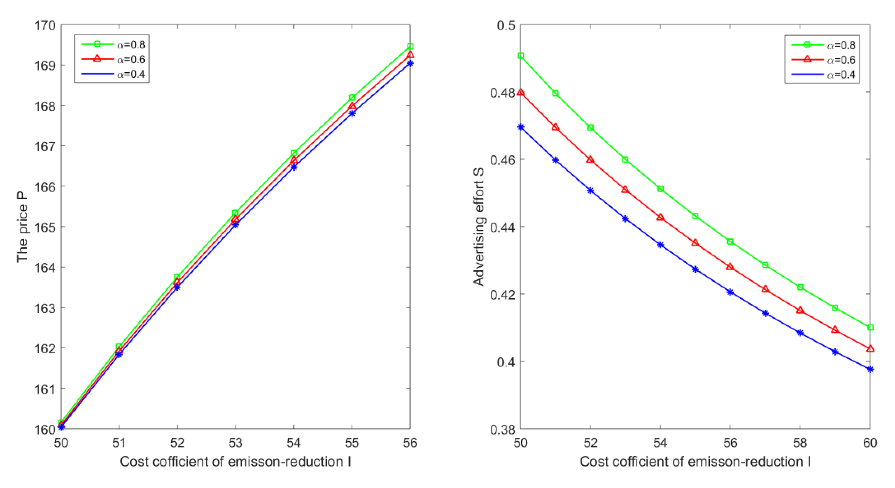
Figure 4.
The impact of Penalty or Subsidy of government on optimal decisions of the retailer.
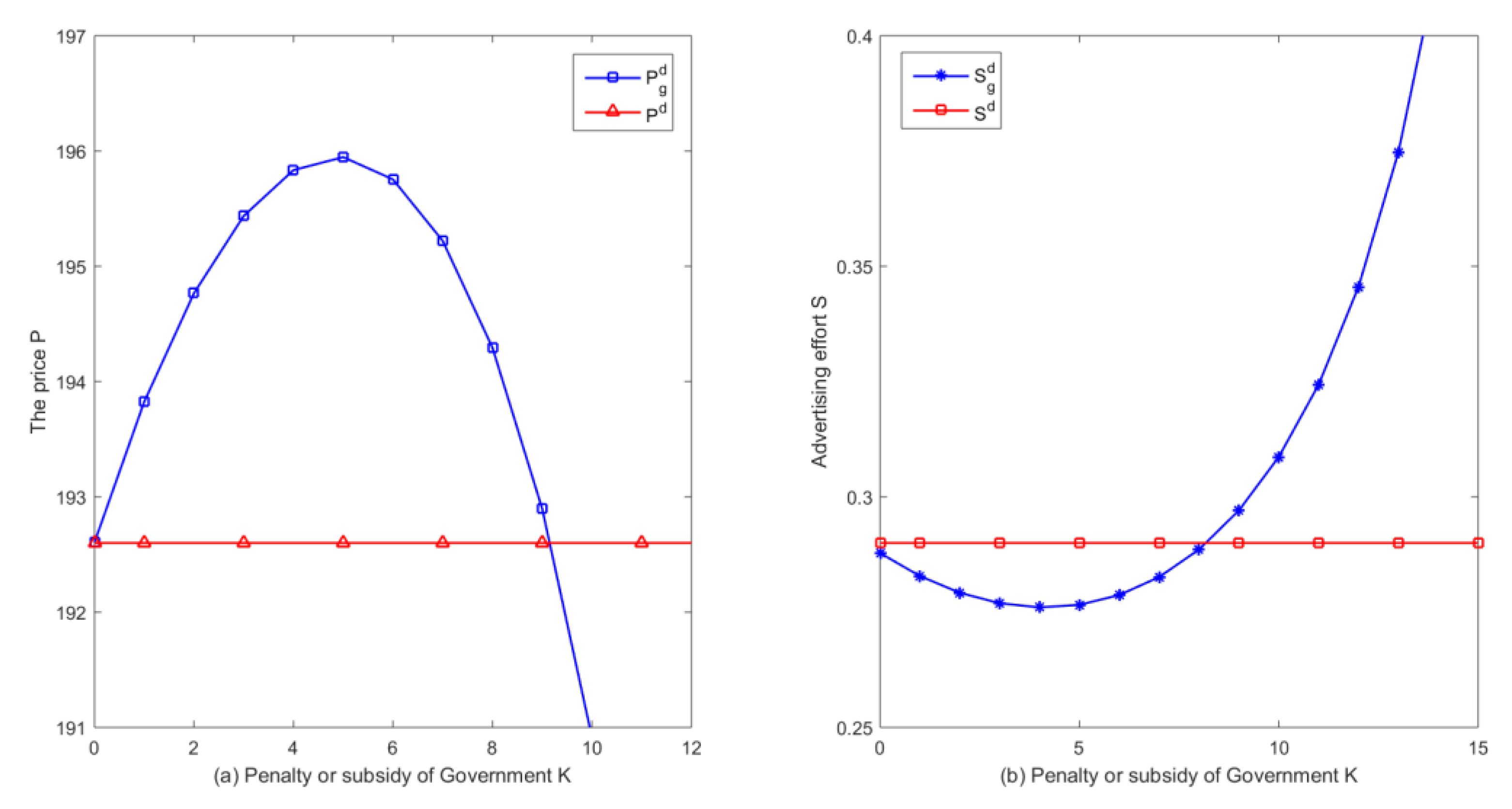
Figure 5.
The impact of on the profit .
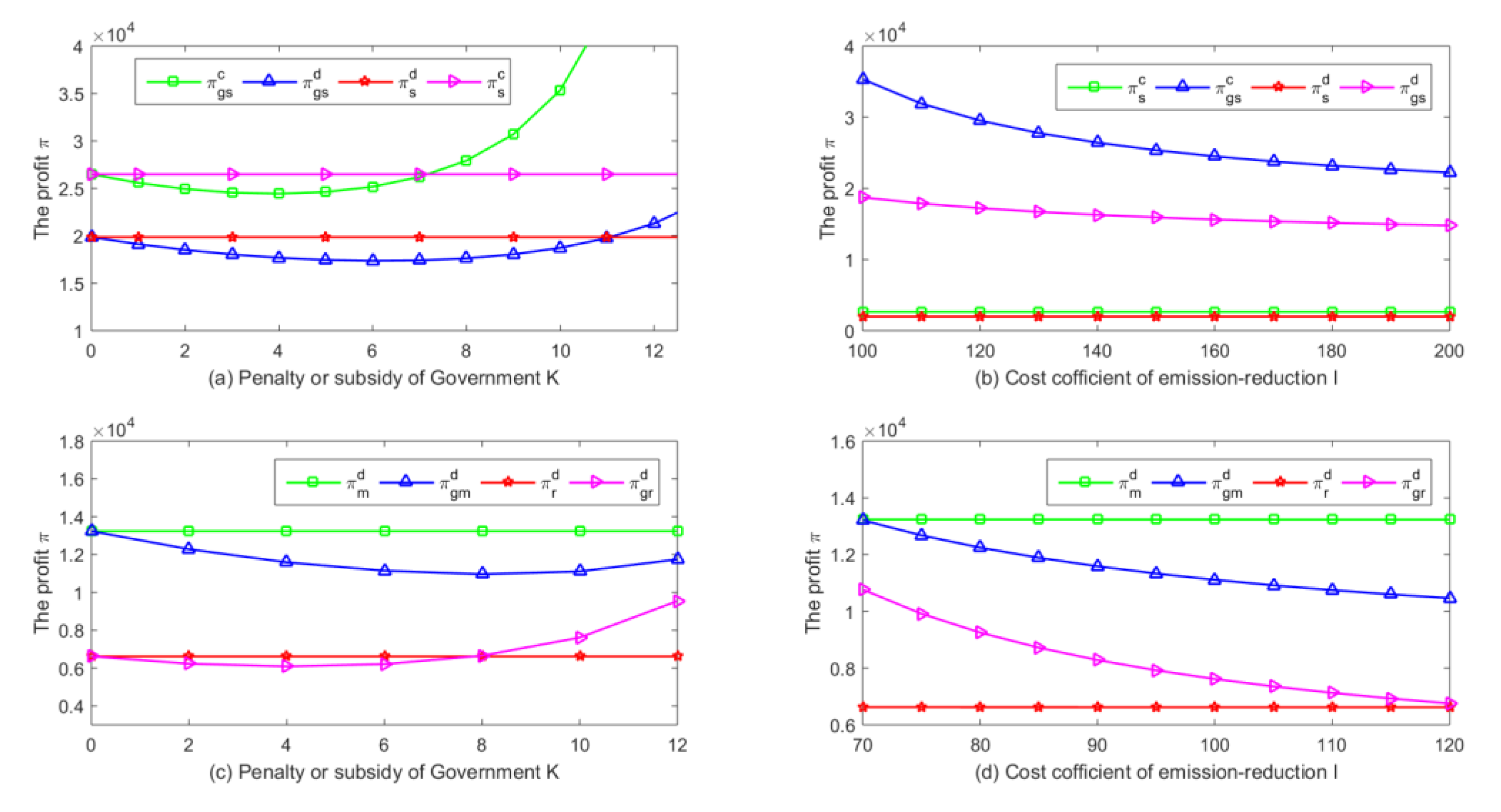
Figure 6.
The impact of on the optimal decisions of the manufacturer and the retailer.
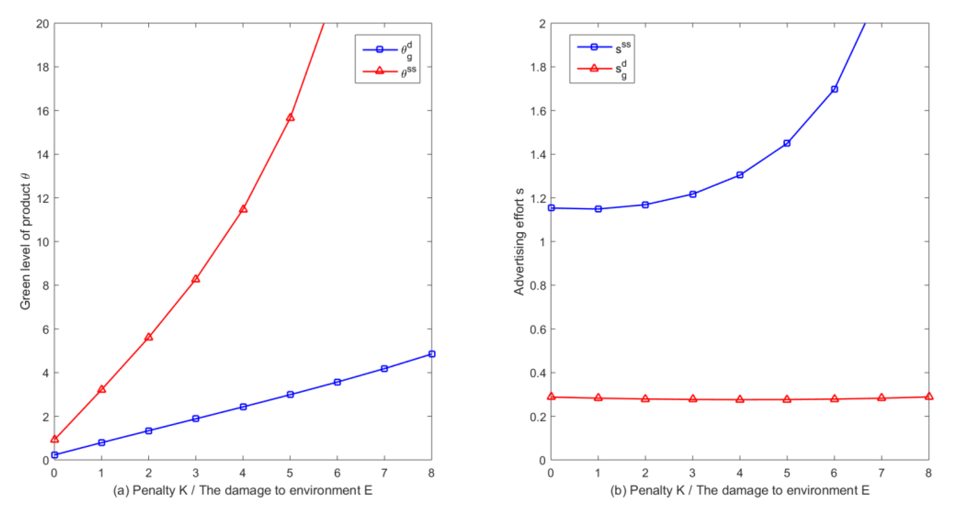
Figure 7.
Change of with proportion under cost-revenue-sharing contract.

Figure 8.
The impact of on the overall profit of supply chain with/without contract.

Table 1.
Notations.
| Parameters | |
|---|---|
| Penalty or subsidy of government for per unit deviation from the standard | |
| Green level standard | |
| Unit production cost (not including emission reduction cost) | |
| Cost coefficient of emission reduction | |
| Potential demand for the product | |
| Consumers’ demand sensitivity of the green level | |
| Consumers’ demand sensitivity of advertising effort | |
| Demand sensitivity of the price | |
| Cost coefficient of advertising effort | |
| Decision variables | |
| Green level of the product | |
| The wholesale price of the product | |
| The unit selling price of the product | |
| Advertising effort of the retailer | |
© 2020 by the authors. Licensee MDPI, Basel, Switzerland. This article is an open access article distributed under the terms and conditions of the Creative Commons Attribution (CC BY) license (http://creativecommons.org/licenses/by/4.0/).
Share and Cite
MDPI and ACS Style
Zhang, W.; Xiao, J.; Cai, L. Joint Emission Reduction Strategy in Green Supply Chain under Environmental Regulation. Sustainability 2020, 12, 3440. https://doi.org/10.3390/su12083440
AMA Style
Zhang W, Xiao J, Cai L. Joint Emission Reduction Strategy in Green Supply Chain under Environmental Regulation. Sustainability. 2020; 12(8):3440. https://doi.org/10.3390/su12083440
Chicago/Turabian StyleZhang, Wensi, Jing Xiao, and Lingfei Cai. 2020. "Joint Emission Reduction Strategy in Green Supply Chain under Environmental Regulation" Sustainability 12, no. 8: 3440. https://doi.org/10.3390/su12083440
Note that from the first issue of 2016, this journal uses article numbers instead of page numbers. See further details here.