Comparative Evaluation of Simplified Surface Energy Balance Index-Based Actual ET against Lysimeter Data in a Tropical River Basin

Abstract

In the past decades, multispectral and multitemporal remote sensing has been popularly used for estimating actual evapotranspiration (ET_c) across the globe. It has been proven to be a cost-effective tool for understanding agricultural practices in a region. Today, because of the availability of different onboard sensors on an increasing number of different satellites, land surface activity can be captured at fine spatial and time scales. In the present study, three multi-date satellite imageries were used for the evaluation of remote sensing-based estimation of actual evapotranspiration in paddy in the command area of the tropical Kangsabati river basin. A surface energy balance model, the Simplified-Surface Energy Balance Index (S-SEBI), was applied for all three dates of the Rabi season (2014–2015) for the estimation of actual evapotranspiration. The crop coefficient was calculated using the exhaustive survey data collected from the command area and adjusted to local conditions. The ET_c estimated using the S-SEBI-based model was compared with the Food and Agriculture Organization Penman–Monteith (FAO-56 PM) method multiplied by the adjusted local crop coefficient and lysimeter data in the command area. The coefficient of determination (r²) was applied to examine the accuracy of the S-SEBI model with respect to lysimeter data and the FAO-56 PM-based ET_c. The results showed that the S-SEBI model performed well with the lysimeter (r² = 0.90) in comparison with FAO-56 PM, with an r² of 0.65. In addition to this, the S-SEBI-based ET estimates correlated well with the FAO-56 PM, with r and RMSE values of 0.06 and 1.13 mm/day (initial stage), 0.85 and 0.48 mm/day (development stage), and 0.77 and 0.52 (maturity stage) for paddy, respectively. The S-SEBI-based ET_c estimate varied with different stages of crop growth and successfully captured the spatial heterogeneity within the command area. In general, this study showed that the S-SEBI method has the potential to calculate spatial evapotranspiration and provide useful information for efficient water management. The results revealed the applicability and accuracy of remote sensing-based ET for managing water resources in a command area with scarce data.

1. Introduction

Monitoring the spatial and temporal variation of actual evapotranspiration of agricultural crops helps in making future decisions (e.g., about water management and crop management) at the macro-level, particularly in rainfed agriculture. In rainfed areas, variability in cropping is very closely related to irregular rainfall. This type of study is very critical for water-limited environments because in these regions, evapotranspiration is a dominant factor in water balance [1,2]. Authentic information on different types of crops cultivated in the command area is very crucial to water managers for releasing water in the command area. Spatial information on water consumption in irrigated areas is very important for ameliorating water productivity [3,4,5,6]. Evapotranspiration (ET) is a fundamental process of the hydrological cycle in which the evaporation of water takes place from the land surface, and transpiration occurs from the canopy cover [7]. Evapotranspiration (ET) is a critical parameter for improving water productivity. Precise monitoring of ET in a catchment is required to improve the water productivity in the command area. ET is computed using the water balance approach in field experiments or indirectly from climatic parameters from the weather station. In addition to this, ET is spatial–temporal in nature for a heterogeneous area, which makes it impossible to compute ET for large areas with ground observation data [8,9].

Remote sensing provides authentic and coherent time series data for collecting the required information to map crop type and acreage. In addition to this, it provides large coverage [10,11]. Remote sensing can provide additional information regarding crop health. The spectral reflectance of a crop changes with respect to crop type, stage, and health. Information from the satellite image can be extracted by inputting satellite imagery combined with ancillary data to provide information for the management of the agricultural farm [12,13]. The use of remote sensing for calculating the crop area has a long history beginning in the 1970s [14]. The requirement of timely and authentic information for tactical and future decision-making in agricultural practices, such as crop identification, crop water requirements, and the calculation of evapotranspiration is very important for efficient management. Remotely sensed data can be used for drought identification and flood damage assessment [15,16,17]. However, the most important limitation on crop identification using satellite imagery, such as cloud cover in Kharif season, matching the reflectance of different plants, small agricultural field size, and differences in the patterns of individual crop phenology.

With the advancement in remote sensing technology, ET can be measured indirectly from satellite imagery using a set of equations in strict hierarchical steps to convert spectral radiance into actual ET. The development of remote sensing technology to estimate actual ET indirectly from satellite imagery has radically transformed our abilities in the area of water resource management [12,14]. Satellite imagery is an excellent source of consistent and frequent observation of the land surface in near-real time [18,19]. Several researchers [20,21,22,23] across the world have developed different algorithms for ET, making use of remote sensing data obtained from satellite imagery or unmanned aerial vehicles (UAV). Remotely sensed data are best for computing ET from seamless heterogeneous crop fields using the surface energy balance technique. There are different field-based instruments used for estimating ET, viz., Lysimeter, Eddy covariance, Bowen Ratio Energy Balance Systems (BREBS), and scintillometers [24,25].

However, these methods are pertinent for local scales, and their interpolation to a large area does not represent the spatial dynamics of heterogeneous conditions. Numerous researchers across the globe have reported that remote sensing technology has shown immense potential for the monitoring and quantification of spatial–temporal variation of ET because of its synoptic and repetitive capabilities. The two most popular remote sensing-based ET estimation approaches are (a) the vegetation index-based approach, which is based on the relationship between the vegetation index (VI) and the crop coefficient, and (b) the surface energy balance approach, which is based on the thermal remote sensing data.

The advantages of remote sensing-based ET estimation over the conventional method can be summarized as (a) the large area coverage and availability of freely remote sensing data; (b) all stakeholders related to water are included; (c) historical data are available; and (d) near-real-time assessment of ET can be conducted. Several researchers across the world have reported the applicability of remote sensing-based ET estimation for efficient water management. However, in heterogeneous and composite areas, point estimates are not sufficient, and the quantification of actual evapotranspiration is a complex and challenging task. Hence, it is crucial to explore the estimation of actual evapotranspiration using the remote sensing-based surface energy balance approach. Remote sensing-based ET estimation plays an important role in water resource management in the command area. Thus, the quantification of actual ET and its spatial distribution is of prime importance for managing water resources in a catchment.

In the present research study, an effort was made to utilize the remote sensing-based ET algorithm to compute ET_c in a command area using different models and its comparison with lysimeter data. The research used Landsat 8 imagery by applying the remote sensing-based crop coefficient vegetation index by incorporating fractional vegetation cover to calculate the actual ET of paddy in an agricultural-dominated catchment in India. To our knowledge, very few studies in the context of India have reported the evaluation of ET computed using S-SEBI and its validation against lysimeter data. The major highlights of the present research paper are that it utilizes exhaustive survey data with detailed descriptions regarding the sowing date, name of the crop, crop height at different stages, and latitude and longitude of the survey location at different times during the crop season. This study utilized lysimeter data to evaluate satellite-based ET estimation models. The objectives of the present research were (a) to estimate ET_c using the remote sensing-based surface energy balance approach, i.e., S-SEBI, using Landsat 8 imagery and (b) to compare and validate S-SEBI-based ET with lysimeter ET data available in the study area. The present study illustrates the potential of remote sensing data to map ET at the command scale for efficient water management practices.

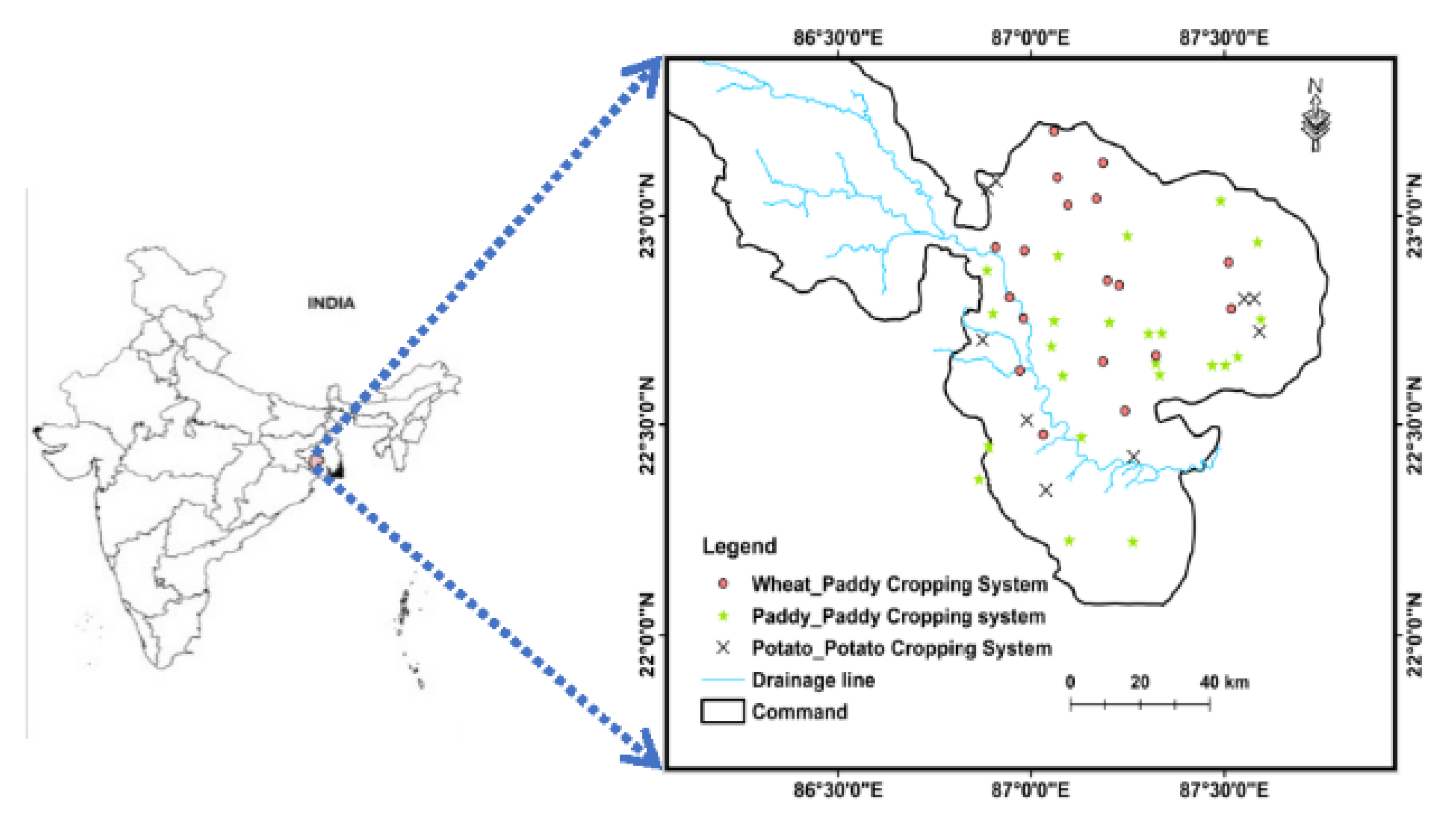
2. Project Site Description and Data Used

The project site (Figure 1) considered for the current research was the Kangsabati Command Area (KCA), a tropical river basin situated in the West Bengal state of India. The geographical extent of KCA extends from longitude 86° E–87°30′ E to latitude 22°20′ N–23°30′ N. The mean annual precipitation of the command area is 1400 mm, which is the average from five rain gauges lying inside the Kangsabati river basin. About 80% of rainfall is received over four months (June to September) of the southwest summer monsoon. The Kangsabati reservoir basin is considered drought-prone in the upstream region because of its higher elevation and lateritic soil, which leads to high runoff. Paddy is the dominant crop grown in the command area.

3. Remotely Sensed Data

The remotely sensed data used in the present study were acquired from the United States Geological Survey (USGS) website https://earthexplorer.usgs.gov/ accessed on 26 September 2020) for the Rabi season of 2014–2015 (December to March). Three multi-date multispectral and thermal remote sensing data from the Landsat 8 Operational Land Imager (OLI)/Thermal Infrared Sensor (TIRS) satellite imagery were used in this research. It comprised a spatial resolution of 30 m in the optical band and 100 m disaggregated to 30 m in the thermal band with a 16-day revisit period. Attention was given when selecting satellite imagery that it did not have cloud coverage of more than 10%. Only three images were found fulfilling the above-mentioned condition during the study period. The description of remote sensing imagery is given in

Table 1. List of Landsat 8 imagery used in the study.

Path	Row	Sensor	Spatial Resolution	Date
139	44	Operational Land Imager (OLI), Thermal Infrared Sensor (TIRS)	30 m, 100 m (resample to 30 m)	10 January 2015, 27 February 2015, 15 March 2015

.

4. Survey Data for Crop Coefficient Vegetation Modeling

Survey data for crop coefficient vegetation modeling were collected from 100 survey points for Rabi season (2014–2015) in December–October covering the Kangsabati Command Area (KCA). Survey data points were collected from a large field of homogenous land use/land cover (LULC). Survey data included facts such as land use categories, crop type, sowing date, crop height, irrigation source, and latitude and longitude of the field using a global positioning system (GPS). The typical information for a survey location is given in Figure 2 along with a picture of the crop at the survey time. Attempts were made to select the survey date coinciding with the satellite visit period.

5. Meteorological Data

Daily climatic parameters, such as the maximum temperature, minimum temperature, and precipitation, were taken from the automatic meteorological station situated in the Agricultural and Food Engineering (AgFE) Department, which lies in the study area. Climatic parameters were collected from December to March (2014–2015) for the calculation of reference evapotranspiration.

6. Methodology

6.1. Computation of Surface Energy Fluxes from Landsat 8 Imagery

In order to implement S-SEBI for estimating ET_c, several input model parameters needed to be calculated.

Table 2. Crop coefficient (K_c) and modified crop coefficient (Mod_Kc) values for paddy crop in the selected study area.

Growth Stage	Paddy
	FAO Kc	10 January 2015	27 February 2015	15 March 2015
		Mod_Kc
Initial	1.00	1.00	1.00	1.00
Development	1.15	1.18	1.13	1.12
Maturity	0.70	0.80	0.72	0.71

displays the mathematical expressions applied to compute the normalized difference vegetation index (NDVI), surface albedo (α), transmissivity of atmosphere (τ_sw), net radiation (R_n), net incoming shortwave radiation (RS↓), entering long wave radiation (RL↓), and departing long wave radiation (RL↑). The equations used for calculating different S-SEBI input parameters were applied for all three dates to obtain various parameters for calculating instantaneous latent heat flux, which was subsequently converted in actual ET. The fundamental equation of ET estimation based on the surface energy balance approach is given by [26,27]:

R_n = G + H + λE

(1)

Equation (2) can be rewritten as:

λE = R_n − G − H

(2)

To check the reliability of the associated fluxes using the energy balance closure, Λ at any time during the day can be computed using Equations (3) and (4) and can be written in the following form [28]:

H + λE = Λ (R_n − G)

(3)

6.2. Estimation of Surface Energy Flux Using Landsat 8

6.2.1. Net Radiation

The net radiation (R_n) can be computed as [29]:

$$R_n=\left(1-\alpha \right)RS\downarrow +RL\downarrow -RL\uparrow -\left(1-{\mathsf{\epsilon }}_0\right)RL\downarrow$$

(4)

The net short-wave radiation (R_si) was determined using Equation (5):

R_si = G_sec × cos θ × τ_sw

(5)

where α = surface albedo, G_sec = solar constant (W/m²), θ = (90° − θ_SE) is the angle of solar incidence, θ_SE is the sunset hour angle, and τ_sw = transmissivity of atmosphere.

For any clear-sky day, τ_sw can be determined as [30]:

τ_sw = 0.75 + 2 × 10⁻⁵ (h)

(6)

where h is the surface height (m).

The normalized difference vegetation index (NDVI) is the ratio of the difference between the near-infrared (ρ_NIR) and red (ρ_R) reflectance divided by their sum [31,32,33]:

$$NDVI=\frac{{\rho }_{NIR}-{\rho }_R}{{\rho }_{NIR}+{\rho }_R}$$

(7)

where ${\rho }_R$ = reflectance of the red band and ${\rho }_{NIR}$ = reflectance of the near-infrared band.

The land surface emissivity (${ϵ}_{\lambda }$) was calculated based on the NDVI threshold method [34,35]:

$${ϵ}_{\lambda }=\left\{\begin{array}{c}{a}_{\lambda }+b_{\lambda }{\rho }_R NDVI<{NDVI}_S\\ {\epsilon }_{V\lambda }{p}_V+{\epsilon }_{S\lambda }\left(1-p_V\right)+C_{\lambda } NDVI\le NDVI<{NDVI}_V\\ {\epsilon }_{V\lambda }{p}_V+C_{\lambda }NDVI>NDV{I}_V\end{array}\right\}$$

(8)

where ${\epsilon }_{V\lambda }$ and ${\epsilon }_{S\lambda }$ are the emissivity of vegetation and soil, respectively; $a_{\lambda }$ and $b_{\lambda }$ are the parameters retrieved from metadata of particular Landsat 8 imagery; $C_{\lambda }$ represents surface roughness ($C_{\lambda }$ = 0 for a plane surface); and $p_V$ is the partial vegetation computed using Equation (9) [33]:

$$P_v={\left(\frac{NDVI-{NDVI}_s}{{NDVI}_v-{NDVI}_s}\right)}^2$$

(9)

where NDVI_v and NDVI_s are the threshold NDVI_s for healthy vegetation and a dry soil pixel, respectively, evaluated from the NDVI histogram. If NDVI is greater than NDVI_v, a numerical value (0.985) is used for emissivity [34].

There are many algorithms devised to calculate the LST from the thermal infrared (TIR) band of Landsat 8 imagery. We adopted the methodology of [35] to compute the surface radiometric temperature (T_s).

RL ↓ is the downward long wave radiation reflected from the atmosphere, calculated as:

$$RL\downarrow ={\epsilon }_a\times \sigma \times T_a^4$$

(10)

where T_a = near-surface air temperature (K) and ${\epsilon }_a$ = atmospheric emissivity, calculated as [36]:

$${\epsilon }_a=0.85\times {\left(-\ln \left({\tau }_{sw}\right)\right)}^{0.09}$$

(11)

$RL\uparrow$ is computed using Equation (12):

$$RL\uparrow ={\epsilon }_0\times \sigma \times T_s^4$$

(12)

6.2.2. Soil Heat Flux (G)

Soil heat flux was calculated using the semi-empirical relationship between net radiation, surface albedo, surface temperature, and NDVI [37]:

$$\frac{G}{R_n}=\frac{T_s}{\alpha }\left(0.0038\alpha +0.0074{\alpha }^2\right)\left(1-0.98{NDVI}^4\right)$$

(13)

The daily soil heat flux can be taken to be zero, as the land gives out the heat that it absorbs during the day.

6.3. Evaporative Fraction (Λ)

The simplified form of the surface energy balance approach, called S-SEBI, was implemented in this research study to calculate the surface flux from satellite imagery data. The diurnal variation of the evaporative fraction was incorporated in the evaporative fraction. The value of the evaporative fraction (Λ) was obtained using a two-dimensional scatter plot of the land surface temperature (LST) and albedo for each Landsat 8 imagery [38]:

$$\mathsf{\Lambda }=\frac{T_H-T_s}{T_H-T_{\lambda E}}$$

(14)

where T_s = LST (K); T_H and T_λE are computed using the regression equation developed as a function of surface albedo as follows:

$$T_H=a+b\times \alpha$$

(15)

$$T_{\lambda \mathrm{E}}=b+c\times \alpha$$

(16)

where a, b, c, and d are empirical constants calculated from the scatter plot between LST and surface albedo. The value of the evaporative fraction for each pixel is calculated using Equation (14).

6.4. Estimation of Actual ET Using S-SEBI

The variation in surface albedo reflectance between the highest and lowest temperatures for hot and cold surroundings, respectively, is the foundation of the S-SEBI model. It is used as the basic principle to partition sensible and latent heat fluxes. If the imagery under study contains hot and cold pixels, no additional meteorological data is required to estimate ET. The S-SEBI method can be implemented if the surface extremes, i.e., hot and cold pixels, are present in the image. The main advantages of the S-SEBI model are that (1) no meteorological data are needed to derive the evaporative fraction if hot and cold pixels are present in the imagery and (2) the maximum and minimum temperatures for hot and cold pixels change with a change in reflectance value. On a daily basis, the contribution of ground heat flux (G, W/m²) can be considered negligible, and (R_n − G) can be written as (R_n, W/m²). The daily ET_c (mm/day) can be computed using the S-SEBI model as suggested by [39,40]:

$${ET}_c=\frac{\ast {10}^3}{{\lambda \ast \rho }_w}{\Lambda R}_n$$

(17)

where λ = latent heat of vaporization (J/kg), Λ = evaporative fraction, and ${\rho }_w$ = the density of water (kg/m³).

6.5. Calculation of Reference ET

The reference ET was calculated using the Penman–Monteith model from climate data available from a nearby weather station available in the command area. Crop evapotranspiration was calculated as [36]:

$${ET}_c=K_c\times {ET}_o$$

(18)

Different equations have been developed to estimate ET_o across the globe in different agro-climatic zones, which have been extensively evaluated using lysimeter data. However, the standard and reliable method for computing ET_o is the FAO Penman–Monteith method. In the present study, we used the FAO Penman–Monteith method to calculate ET_o. The reference ET was computed using the climatic parameters and represents the response of the climatic parameters to environmental conditions. K_c is different for different crops and represents the crop canopy development and crop management practices throughout the growing season. The FAO-56 PM method was used as the standard method in the present research:

$$E{T}_o=\frac{0.408\left(R_n-G\right)+\frac{900}{T_a+273}{u}_2\left(e_s-e_a\right)}{\Delta +\gamma \left(1+0.34\mathrm{u}\right)}$$

(19)

where ET_o is the potential reference crop evapotranspiration (mm ${\mathrm{day}}^{-1}$); $R_n$ is the total incoming solar radiation (MJ ${\mathrm{m}}^{-2}{\mathrm{day}}^{-1}$); G is the ground heat flux (MJ ${\mathrm{m}}^{-2}{\mathrm{day}}^{-1}$), which is taken as nil on daily basis; $T_a$ is the mean daily temperature ($°C$); u₂ is the wind speed at a height of 2 m (m ${\sec }^{-1}$); $e_s$ is the vapor pressure deficit at saturation (kPa);$e_s$ is the vapor pressure deficit of actual air (kPa); $e_s-e_a$ is the difference in the vapor pressure deficit (kPa); $\Delta$ is the tangent of the saturation vapor pressure–temperature curve (kPa ${°C}^{-1}$); and $\gamma$ is the psychometric constant (kPa ${°C}^{-1}$).

6.6. Performance Indicator

The estimated ET_c calculated on the basis of the S-SEBI was compared with the ET_c observed from lysimeter data using linear regression. Correlation analysis was applied to examine the goodness of fit between the actual and predicted ET_c values. The coefficient of determination (r²), root-mean-squared error (RMSE), correlation coefficient (r), mean squares error (MSE), and index of agreement (d) were used as a relative index for the model performance [41]. The r², RMSE, r, d, and MSE were estimated as:

$$r^2=1-\frac{{\displaystyle \sum }{\left({ET}_{S-SEBI}-{ET}_{Lys}\right)}^2}{{\displaystyle \sum }{\left({ET}_{Lys}-{ET}_{Mean}\right)}^2}$$

(20)

$$RMSE=\sqrt{\frac{1}{n}{\displaystyle \sum }_{i=1}^n{\left[E_i\left(l\right)-{\widehat{E}}_i\left(l\right)\right]}^2}$$

(21)

$$r=\frac{{{\displaystyle \sum }}_{l=1}^n\left(E_i\left(l\right)-{\overline{E}}_i\right)\left({\widehat{E}}_i\left(l\right)-{\overline{\widehat{E}}}_i\right)}{\sqrt{{{\displaystyle \sum }}_{l=1}^n{\left(E_i\left(l\right)-{\overline{E}}_i\right)}^2{{\displaystyle \sum }}_{t=1}^n{\left({\widehat{E}}_i\left(l\right)-{\overline{\widehat{E}}}_i\right)}^2}}$$

(22)

$$d=1-\left(\frac{{{\displaystyle \sum }}_{i=1}^n{\left(E_i\left(l\right)-{\widehat{E}}_i\left(l\right)\right)}^2}{{\left(\left({{\displaystyle \sum }}_{i=1}^n\left|{\widehat{E}}_i\left(l\right)-E_{imean}\left(l\right)\right|+{{\displaystyle \sum }}_{i=1}^n\left|E_i\left(l\right)-E_{imean}\left(l\right)\right|\right)\right)}^2}\right)$$

(23)

$$MSE=\frac{1}{n}{\displaystyle \sum }_{i=1}^n{\left(E_i\left(l\right)-{\widehat{E}}_i\left(l\right)\right)}^2$$

(24)

where ${ET}_{Lys}$ is the observed ET_c (mm/day) values from the lysimeter, ${ET}_{S-SEBI}$ is the mean value of the estimated ET_c (mm/day) at different crop growth stages using the S-SEBI model, ${\widehat{E}}_i\left(l\right)$ is the estimated ET using the S-SEBI at the ith crop location, $E_i\left(l\right)$ is the estimated ET using the crop-coefficient-coupled FAO56 Penman–Montieth method at the ith crop location, and N is the total number of selected locations of paddy for respective comparison.

7. Results and Discussion

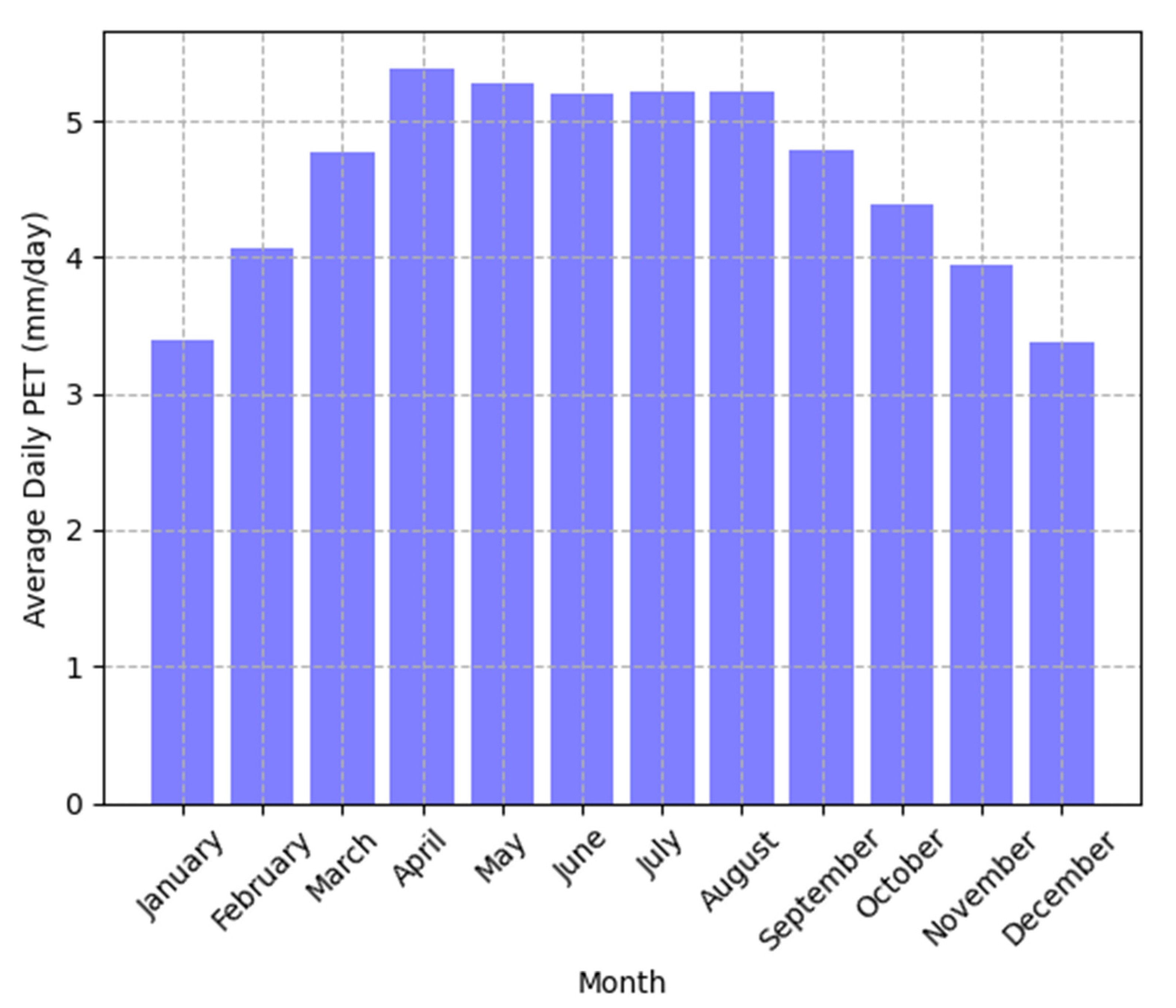
7.1. Seasonal Variation of ET_o

The climate data collected from the weather station located in the AgFE farm were used to calculate the reference ET_o using a decision support system (DSS-ET). The total ET_o was 1102 mm in a year, while the cumulative ET during the study period was found to be 1105 mm. The time-series variation of the average monthly daily ET_o is presented in Figure 3. The average monthly daily ET_o increased from January and then decreased until December. The maximum average daily ET_o was found in the month of June.

7.2. Temporal Variation of NDVI

The temporal distribution of NDVI for the study period over KCA was generated using Landsat 8 time series and survey points collected from the large fields, detailed survey information, and irrigation sources. The typical spectrum for paddy crops is presented in Figure 4. The rising part of the NDVI profile curve marks the initial stage of crop growth. From the temporal NDVI profile, it is clear that for paddy, the germination period was in mid-December. The peak of the NDVI time series occurred in mid–late February for wheat. The maturity of the crop was seen in late March. Exhaustive survey data regarding crop information for obtaining spectral signatures were applied in the present study.

7.3. Spatial–Temporal Variation of NDVI over Study Region

The spatial variation indicated that the value of NDVI increased as the season progressed. Spatial–temporal maps of NDVI were generated using the near-infrared and red bands from Landsat 8 imagery. The mean value of NDVI for the different growth stages of the crop was calculated using the survey point for the paddy crop. These values were further utilized for the development of the crop coefficient vegetation regression model. The NDVI value ranged from 0.2 to 0.5 throughout the growing season; the lower value corresponded to the initial crop growth stage, while the maximum value corresponded to the mid-season stage.

7.4. Calculation of Tabulated Crop Coefficient Value to Local Condition

Different types of parameters and characteristics were utilized to determine the crop coefficient, which included the date of sowing, harvesting, variety of the crop, and development stages [23]. All this information was collected by the field survey conducted by National Remote Sensing Centre (NRSC), Hyderabad, India for the period from November 2014–March 2015 in the Rabi season. These intensive field surveys were conducted at 100 locations in the study area, which allowed the precise validation and estimation of ET [42,43]. Further, the crop coefficient for the basin was calculated by modifying the baseline FAO-56 method [5,23] as follows:

$$K_{c\left(\mathrm{modified}\right)}=K_{c\left(\mathrm{table}\right)}+\left[0.04\left(u_2-2\right)-0.004\left({\mathrm{RH}}_{\min }-45\right)\right]{\left(\frac{h}{3}\right)}^{0.3}$$

(25)

where K_c (modified) is the modified K_c based on the FAO-56 method, K_c (table) values are values determined from Table 12 provided in the manual of FAO-56 [7], h defines the height of the crop at a given stage (m) for 0.1 m < h < 10 m, u₂ is the wind speed at a 2 m height, and RH_min is minimum relative humidity (%) for 20% ≤ RH_min ≤ 80%. Table 2 shows the adjusted local crop coefficient value using the above equation.

7.5. Spatial–Temporal Variation of ET over Study Area

The spatial variation of actual ET estimated using the S-SEBI-based approach is shown in Figure 5. Actual ET over the study area varied during the crop growth season. It was low during the initial growth stage, increased during the crop growth stage, and then decreased to the crop maturity stage. The average value of actual ET for different crop stages was calculated using the mean of actual ET for all survey points belonging to the same crop. The spatial variation showed the evaporative pattern over the whole command. As the crop season progressed from the crop’s initial stage to the maturity stage, the area with low ET_c increased, as seen from the spatial ET_c derived using the S-SEBI method. This indicates that the S-SEBI-based ET estimate was able to capture the crop phenology well during the crop growth cycle.

7.6. Lysimeter ETc

To validate the S-SEBI-based actual ET, a plot-scale lysimeter was installed in the experimental field of the Agriculture and Food Engineering Department, Indian Institute of Technology, Kharagpur (23°32′ N; 87°31′ E), during the Rabi (winter) seasons. Four numbers of open-bottom and two numbers of closed-bottom non-weighing lysimeters with/without paddy crops, with dimensions of 1.25 × 1.25 × 1 m, were used. A combination of volumetric water balances in the open-bottom and closed-bottom lysimeters was used to determine the daily crop evapotranspiration (ET_c). Subsequently, the daily crop coefficients were estimated by dividing ET_c by the FAO56 PM-derived ET_o for each of the four different growth stages of the paddy crop. The values of the crop coefficient for stages 1, 2, 3, and 4 were 0.85, 0.995, 1.1, and 0.8 for the Rabi season, respectively.

7.7. Validation of S-SEBI ETc

Lysimeter- and FAO-56 Penman–Monteith-derived ET were used to evaluate S-SEBI-based ET. The average value of actual ET in all paddy locations was calculated for different crop growth stages and compared corresponding to the lysimeter value observed at the experimental AgFE farm located in IIT Kharagpur. Similarly, S-SEBI-based ET was also evaluated against the FAO-56 Penman–Monteith model, which is internationally recognized. The scatter plot of S-SEBI-based ET with respect to lysimeter data and the FAO-56 Penman–Monteith model is shown in Figure 6. ET computed using the S-SEBI showed strong agreement with lysimeter data. The r and RMSE value for paddy was found to be better during the development stage (0.85, 0.48 mm/day) than during the initial stage (0.06, 1.13 mm/day) and the maturity stage (0.77, 0.52 mm/day).

Table 3. Summary of comparative performance of ET_c_S-SEBI with respect to FAO-56 PM for different locations of paddy crop.

Crops	Date	Pearson’s r	p-Value	MSE	RMSE	d
Paddy	10 January 2015	0.06	0.89	1.29	1.13	0.37
	27 February 2015	0.85	0.009	0.25	0.48	0.73
	15 March 2015	0.77	0.007	0.28	0.52	0.68

shows the statistical parameters for the different growth stages of paddy in the study area. The indices of agreement were 0.37, 0.73, and 0.68 for paddy during the initial stage, crop development stage, and maturity stage, respectively. In this study, the crop coefficient-coupled FAO-56 PM method was improved with the inclusion of the modified crop coefficient using the exhaustive survey data. The summary of S-SEBI-based ETc with respect to FAO-56 PM for different locations of paddy crop is shown in Table 3. The results obtained in the present study are in line with a similar study [44] for paddy and wheat crops, respectively, in the TSMC irrigation command (West Bengal, India) and [45] the Mahi river irrigation command (Gujarat, India). The findings of this study are corroborated by [6,46,47,48,49,50,51], in which ET estimation was performed using MODIS and Landsat 8 satellite-based products.

8. Conclusions

The present research provides a comparative assessment of S-SEB-based ET_c with lysimeter data and FAO-56 PM for a fine resolution satellite image, such as Landsat 8, which can be used to monitor irrigation water use over command scales. The key results and the conclusions are summarized below:

1.

Seasonal variations in the NDVI were shown to indicate the vegetation response toward the rainfall for the available data period. The study developed a vegetation index-based crop coefficient model, which is based on a simple linear regression approach.

2.

The study calculated the crop coefficient from the field information collected from survey data. The location-wise ET was calculated from the product of the reference ET calculated from FAO-56 PM and the crop coefficient calculated from survey data. The crop actual evapotranspiration was generated spatially and temporally using remote sensing data.

3.

A spatial and temporal map of ET was obtained on the basis of the evaluation of satellite-based ET with the lysimetric data, which showed good performance in capturing the seasonality.

4.

This research found that the ET_c estimated using the remote sensing-based S-SEBI approach showed good performance (r² = 0.90). Furthermore, it is noticeable that the spatial resolution in the TIR sensor of Landsat 8 imagery is not properly suitable to represent the test site for the validation of ET. The S-SEBI is a simplified model of the surface energy balance approach that depends less on a complicated input model that can adequately capture the spatial evaporative demand and reproduce the daily ET map for the study area. Therefore, the S-SEBI can be applied to compute ETc agriculture land use with better accuracy, and thus the S-SEBI can be operationally implemented for computing ET_c using remotely sensed data with a thermal band for efficient water management and irrigation scheduling. This study concludes that the estimation of ET_c using the remote sensing-based S-SEBI model using exhaustive survey data offers a powerful tool for near-real-time ET_c calculation for irrigation water management in data-scarce regions.

References

1. Abrahams, A.D.; Parsons, A.J. Geomorphology of Desert Environments; Chapman and Hall: London, UK, 1994. [Google Scholar]
2. Gowda, P.H.; Chavez, J.L.; Colaizzi, P.D.; Evett, S.R.; Howell, T.A.; Tolk, J.A. ET mapping for agricultural water management: Present status and challenges. Irrigat. Sci. 2008, 26, 223–237. [Google Scholar] [CrossRef] [Green Version]
3. Bastiaanssen, W.G.M.; Menenti, M.; Feddes, R.A.; Holtslag, A.A.M. A remote sensing surface energy balance algorithm for land (SEBAL): 1. Formulation. J. Hydrol. 1998, 212, 198–212. [Google Scholar] [CrossRef]
4. Goward, S.N.; Markham, B.; Dye, D.G.; Dulaney, W.; Yang, J. Normalized difference vegetation index measurements from the advanced very high resolution radiometer. Remote. Sens. Environ. 1991, 35, 257–277. [Google Scholar] [CrossRef]
5. Glenn, E.P.; Neale, C.M.U.; Hunsaker, D.J.; Nagler, P.L. Vegetation index-based crop coefficients to estimate evapotranspiration by remote sensing in agricultural and natural ecosystems. Hydrol. Process. 2011, 25, 4050–4062. [Google Scholar] [CrossRef]
6. Srivastava, A.; Sahoo, B.; Raghuwanshi, N.S.; Singh, R. Evaluation of Variable Infiltration Capacity model and MODIS-Terra satellite-derived grid-scale evapotranspiration estimates in a river basin with tropical monsoon-type climatology. J. Irrig. Drain. Eng. 2017, 143, 04017028. [Google Scholar] [CrossRef] [Green Version]
7. Allen, R.G.; Pereira, L.S.; Raes, D.; Smith, M. Crop Evapotranspiration–Guidelines for Computing Crop Water Requirements-FAO Irrigation and Drainage Paper 56; FAO: Rome, Italy, 1998; 300p. [Google Scholar]
8. Kumar, U.; Sahoo, B.; Chatterjee, C.; Raghuwanshi, N. Evaluation of simplified surface energy balance index (S−SEBI) method for estimating actual evapotranspiration in Kangsabati reservoir command using landsat 8 imagery. J. Indian Soc. Remote. Sens. 2020, 48, 1421–1432. [Google Scholar] [CrossRef]
9. Senay, G.B.; Friedrichs, M.; Singh, R.K.; Velpuri, N.M. Evaluating Landsat 8 evapotranspiration for water use mapping in the Colorado River Basin. Remote. Sens. Environ. 2016, 185, 171–185. [Google Scholar] [CrossRef] [Green Version]
10. Kumar, U.; Singh, S.; Bisht, J.K.; Kant, L. Use of meteorological data for identification of agricultural drought in Kumaon region of Uttarakhand. J Earth Syst Sci. 2021, 130, 121. [Google Scholar] [CrossRef]
11. Samani, Z.; Bawazir, A.S.; Bleiweiss, M.; Skaggs, R.; Longworth, J.; Tran, V.D.; Pinon, A. Using remote sensing to evaluate the spatial variability of evapotranspiration and crop coefficient in the lower Rio Grande Valley, New Mexico. Irrig. Sci. 2009, 28, 93–100. [Google Scholar] [CrossRef] [Green Version]
12. Murray, R.S.; Nagler, P.L.; Morino, K.; Glenn, E.P. An Empirical Algorithm for Estimating Agricultural and Riparian Evapotranspiration Using MODIS Enhanced Vegetation Index and Ground Measurements of ET. II. Application to the Lower Colorado River, U.S. Remote Sens. 2009, 1, 1125–1138. [Google Scholar] [CrossRef] [Green Version]
13. Kumar, U.; Panday, S.C.; Kumar, J.; Meena, V.S.; Parihar, M.; Singh, S.; Bisht, J.K.; Kant, L. Comparison of recent rainfall trend in complex hilly terrain of sub−temperate region of Uttarakhand. MAUSAM 2021, 72, 349−358. [Google Scholar] [CrossRef]
14. Sharples, J.A. The Corn Blight Watch Experiment: Economic Implications for Use of Remote Sensing for Collecting Data on Major Crops; LARS Technical Reports; Purdue University Publication: West Lafayette, IN, USA, 1973; p. 121. [Google Scholar]
15. Hunsaker, D.J.; Pinter, P.J.; Barnes, E.M.; Kimball, B.A. Estimating cotton evapotranspiration crop coefficients with a multispectral vegetation index. Irrig. Sci. 2003, 22, 95–104. [Google Scholar] [CrossRef]
16. Hunsaker, D.J.; Hendrey, G.R.; Kimball, B.A.; Lewin, K.F.; Mauney, J.R.; Nagy, J. Cotton evapotranspiration under field conditions with CO2 enrichment and variable soil moisture regimes. Agric. For. Meteorol. 1994, 70, 247–258. [Google Scholar] [CrossRef]
17. Kumar, U.; Srivastava, A.; Kumari, N.; Rashmi; Sahoo, B.; Chatterjee, C.; Raghuwanshi, N.S. Evaluation of spatio−temporal evapotranspiration using satellite−based approach and lysimeter in the agriculture dominated catchment. J. Indian Soc. Remote Sens. 2021, 49, 1939–1950. [Google Scholar] [CrossRef]
18. Kustas, W.P.; Norman, J.M.; Schmugge, T.J.; Anderson, M.C. Mapping surface energy fluxes with radiometric temperature. In Thermal Remote Sensing in Land Surface Processes; Quattrochi, D., Luvall, J., Eds.; CRC Press: Boca Raton, FL, USA, 2004; pp. 205–253. [Google Scholar]
19. Bausch, W.C. Soil background effects on reflectance-based crop coefficients for corn. Remote Sens. Environ. 1993, 46, 213–222. [Google Scholar] [CrossRef]
20. Bausch, W.C.; Neale, C.M.U. Crop coefficients derived from reflected canopy radiation: A concept. Trans. ASAE 1987, 30, 703–709. [Google Scholar] [CrossRef]
21. Gontia, N.K.; Tiwari, K.N. Estimation of crop coefficient and evapotranspiration of wheat (Triticum aestivum) in an irrigation command using remote sensing and GIS. Water Resour. Manag. 2010, 24, 1399–1414. [Google Scholar] [CrossRef]
22. Johnson, L.F.; Trout, T.J. Satellite NDVI assisted monitoring of vegetable crop evapotranspiration in California’s San Joaquin Valley. Remote Sens. 2012, 4, 439–455. [Google Scholar] [CrossRef] [Green Version]
23. Roerink, G.J.; Su, Z.; Menenti, M. S-SEBI: A simple remote sensing algorithm to estimate the surface energy balance. Phys. Chem. Earth Part B Hydrol. Ocean. Atmos. 2000, 25, 147–157. [Google Scholar] [CrossRef]
24. Doorenbos, J.; Pruitt, W.O. Guidelines for Prediction of Crop Water Requirements; FAO Irrigation and Drainage Paper No. 24 (revised); Food and Agricultural Organization of the United Nations: Rome, Italy, 1977. [Google Scholar]
25. Allen, R.G.; Tasumi, M.; Trezza, R. Satellite-based energy balance for mapping evapotranspiration with internalized calibration (METRIC)-Model. J. Irrig. Drain. Eng. ASCE 2007, 133, 380–394. [Google Scholar] [CrossRef]
26. Jia, L.; Xi, G.; Liu, S.; Huang, C.; Yan, Y.; Liu, G. Regional estimation of daily to annual regional evapotranspiration with MODIS data in the Yellow River Delta wetland. Hydrol. Earth Syst. Sci. 2009, 13, 1775–1787. [Google Scholar] [CrossRef] [Green Version]
27. Kustas, W.P.; Daughtry, C.S.T. Estimation of soil heat flux/net radiation ratio from spectral data. Agric. Forest Meteorol. 1990, 49, 205–223. [Google Scholar] [CrossRef]
28. Liang, S. Narrowband to broadband conversions of land surface albedo I: Algorithms. Rem. Sens. Environ. 2001, 76, 213–238. [Google Scholar] [CrossRef]
29. Menenti, M.; Choudhury, B.J. Parametrization of land surface evapotranspiration using a location dependent potential evapotranspiration and surface temperature range. In Exchange Processes at the Land Surface for a Range of Space and Time Scales; Bolle, H.J., Ed.; IAHS Press IAHS: Wallingford, UK, 1993; pp. 561–588. [Google Scholar]
30. Sobrino, J.A.; El Kharraz, J.; Li, Z.-L. Surface temperature and water vapour retrieval from MODIS data. Int. J. Remote. Sens. 2003, 24, 5161–5182. [Google Scholar] [CrossRef]
31. Rouse, J.W.; Haas, R.H.; Schell, J.A.; Deering, D.W. Monitoring vegetation system in great plains with ERTS. In Proceedings of the 3rd ERTS-1 Symposium, Washington, DC, USA, 10–14 December 1973. GSFC, NASA; SP-351: 48–62. [Google Scholar]
32. Sellers, P.J. Canopy reflectance, photosynthesis, and transpiration. Int. J. Remote. Sens. 1985, 6, 1335–1372. [Google Scholar] [CrossRef]
33. Sobrino, J.A.; Raissouni, N. Toward remote sensing methods for land cover dynamic monitoring. Application to Morocco. Int. J. Rem. Sens. 2000, 21, 353–366. [Google Scholar] [CrossRef]
34. Sobrino, J.A.; Gómez, M.; Jiménez-Muñoz, J.C.; Olioso, A.; Chehbouni, G. A simple algorithm to estimate evapotranspiration from DAIS data: Application to the DAISEX campaigns. J. Hydrol. 2005, 315, 117–125. [Google Scholar] [CrossRef] [Green Version]
35. Sobrino, J.A.; Jiménez-Munoz, J.C.; Sòria, G.; Romaguera, M.; Guanter, L.; Moreno, J.; Plaza, A.; Martínez, P. Land surface emissivity retrieval from different VNIR and TIR sensors. IEEE Trans. Geosci. Remote. Sens. 2008, 46, 316–327. [Google Scholar] [CrossRef]
36. Xu, C.Y.; Singh, V.P. Evaluation of three complementary relationship evapotranspiration models by water balance approach to estimate actual regional evapotranspiration in different climatic regions. J. Hydrol. 2005, 308, 105–121. [Google Scholar] [CrossRef]
37. Kumar, U.; Meena, V.S.; Singh, S.; Bisht, J.K.; Pattanayak, A. Evaluation of digital elevation model in hilly region of Uttarakhand: A case study of experimental farm Hawalbagh. Indian J. Soil Conserv. 2021, 49, 77–81. [Google Scholar]
38. Vyas, S.P.; Oza, M.P.; Dadhwal, V.K. Multi-crop separability study of Rabi crops using multi-temporal satellite data. J. Indian Soc. Remote Sens. 2005, 33, 75–79. [Google Scholar] [CrossRef]
39. Jones, H.G.; Vaughan, R.A. Integrated Applications: Precision Agriculture and Crop Management. In Remote Sensing of Vegetation: Principles, Techniques, and Applications; Oxford University Press: Oxford, UK, 2011; ISBN 978-0199207794. [Google Scholar]
40. Zhou, Y.; Li, X.; Yang, K.; Zhou, J. Assessing the impacts of an ecological water diversion project on water consumption through high-resolution estimations of actual evapotranspiration in the downstream regions of the Heihe River Basin, China. Agric. For. Meteorol. 2018, 249, 210–227. [Google Scholar] [CrossRef]
41. Bastiaanssen, W.G.M.; Ahmad, M.-U.-D.; Chemin, Y. Satellite surveillance of evaporative depletion across the Indus Basin. Water Resour. Res. 2002, 38, 91–99. [Google Scholar] [CrossRef]
42. Sun, Z.; Wei, B.; Su, W.; Shen, W.; Wang, C.; You, D.; Liu, Z. Evapotranspiration estimation based on the SEBAL model in the Nansi Lake Wetland of China. Math. Comput. Model. 2011, 54, 1086–1092. [Google Scholar] [CrossRef]
43. Zwart, S.J.; Bastiaanssen, W.G.M. SEBAL for detecting spatial variation of water productivity and scope for improvement in eight irrigated wheat systems. Agric. Water Manag. 2007, 89, 287–296. [Google Scholar] [CrossRef]
44. Bastiaanssen, W.G.M. SEBAL-based sensible and latent heat fluxes in the irrigated Gediz Basin, Turkey. J. Hydrol. 2000, 229, 87–100. [Google Scholar] [CrossRef]
45. Allen, R.; Irmak, A.; Trezza, R.; Hendrickx, J.M.H.; Bastiaanssen, W.; Kjaersgaard, J. Satellite-based ET estimation in agriculture using SEBAL and METRIC. Hydrol. Process. 2011, 25, 4011–4027. [Google Scholar] [CrossRef]
46. Sun, Z.; Wang, Q.; Matsushita, B.; Fukushima, T.; Ouyang, Z.; Watanabe, M.; Gebremichael, M. Further evaluation of the Sim-ReSET model for ET estimation driven by only satellite inputs. Hydrol. Sci. J. 2013, 58, 994–1012. [Google Scholar] [CrossRef] [Green Version]
47. Mishra, P.; Tiwari, K.N.; Chowdary, V.M.; Gontia, N.K. Irrigation water demand and supply analysis in the command area using remote sensing and GIS. Hydrol J IAH 2005, 28, 59–69. [Google Scholar]
48. Ray, S.S.; Dadhwal, V.K. Estimation of evapotranspiration of irrigation command area using remote sensing and GIS. Agric. Water Manag. 2000, 49, 239–249. [Google Scholar] [CrossRef]
49. Shwetha, H.R.; Kumar, D.N. Estimation of Daily Actual Evapotranspiration Using Vegetation Coefficient Method for Clear and Cloudy Sky Conditions. IEEE J. Sel. Top. Appl. Earth Obs. Remote. Sens. 2020, 13, 2385–2395. [Google Scholar] [CrossRef]
50. Zhang, B.Z.; Xu, D.; Liu, Y.; Li, F.S.; Cai, J.B.; Du, L.J. Multi-scale evapotranspiration of summer maize and the controlling meteorological factors in north China. Agric. For. Meteorol. 2016, 216, 1–12. [Google Scholar] [CrossRef]
51. Danodia, A.; Patel, N.R.; Chol, C.W.; Nikam, B.R.; Sehgal, V.K. Application of S-SEBI model for crop evapotranspiration using Landsat-8 data over parts of North India. Geocarto Int. 2019, 34, 114–131. [Google Scholar] [CrossRef]
Figure 1. Location of project site along with crop system pattern and survey locations.
Sustainability 13 13786 g001
Figure 2. Description of typical survey point along with detailed information.
Sustainability 13 13786 g002
Figure 3. Average daily ETo variation in different months in the study area.
Sustainability 13 13786 g003
Figure 4. Average temporal profile of NDVI for paddy crop extracted from the survey point during the study period.
Sustainability 13 13786 g004
Figure 5. Spatial variation of S-SEBI-based ET during the study period in the command area.
Sustainability 13 13786 g005
Figure 6. Validation of S-SEBI ET with (a) lysimeter data (b) FAO-56 PM ET (mm/day).
Sustainability 13 13786 g006