An Analysis of the Dynamic Relationship between the Global Macroeconomy and Shipping and Shipbuilding Industries

Abstract

Using time-series data from January 2006 to February 2021, this study analyzed the effect of macroeconomic shocks on the shipping and shipbuilding industries. The Granger causality test, recursive structural vector autoregressive models, impulse response analysis, historical decomposition, and local projections model were used to identify the dynamic relationships between the variables and their dynamic effects, based on the results of the theoretical model and previous research. First, the Granger causality test demonstrated that the macroeconomic variables have causal relations with the shipping and shipbuilding industries. Second, the recursive structural vector autoregressive estimation demonstrated that the direction of the shocks from macroeconomic variables is statistically significantly, consistent with the theoretical model. The same results were found in the recursive structural vector autoregressive model and local projection impulse response analysis. Finally, the historical decomposition identified the main causal variables affecting the shipping and shipbuilding industries by period. These findings can help policymakers, operators of shipping and shipbuilding companies, and investors evaluate and make policy-supporting decisions on industry conditions.

1. Introduction

Maritime trade accounts for approximately 80% or more of global trade, indicating that the shipping industry plays a vital role in the global economy [1]. In this respect, shipping demand is derived from global economic demand. Limited research has been conducted on the relationship between the global economy and shipping industry, predominantly by shipping economists, macroeconomists, or economic historians [2]. The first of such studies was conducted by Isserlis [3]; it covered the general process of bulk shipping freight rates from 1869 to World War I and examined the performance between transport volume and freight rates of UK-registered bulk vessels in 1935.

Since then, numerous scholars have examined the role of economic factors in determining freight rates, postulating the key determinants to be industrial production, oil prices, and global economic activity [4,5,6,7]. Kavussanos and Marcoulis [8] applied the multivariate least squares regression method and found that the stock returns of US-listed shipping companies were affected by unexpected changes in macroeconomic factors, such as industrial production and oil prices.

Grammenos and Arkoulis’s [9] study analyzing the relationship between macroeconomic variables and the shipping sector is considered to be significant. It analyzed 36 shipping companies listed on 10 exchange markets and sought to determine the relationship between stock returns and global macroeconomic variables. It noted that oil prices and laid-up tonnage were negatively related to shipping company stock prices, while the exchange rate was positively related to them. Similarly, Kilian [10] argued that real economic activity was associated with bulk carrier shipping and used the bulk carrier freight rate index as a proxy variable for aggregate international demand for crude oil to predict the real economy. Klovland [11] analyzed the relationship between shipping industry business cycles and the global economy and noted that from 1850 to World War II, the global economy was a major determinant of short-term shipping freight rates. In addition, several studies have shown that macroeconomic variables have a significant correlation with fares. These studies have shown that industrial production, among macroeconomic variables, is closely related to shipping freight rates [6,7,12,13,14,15,16].

Also, the focus has been on establishing the macroeconomic variables that affect demand in the shipping industry [12]. In particular, relevant studies have demonstrated that variables that closely indicate the global economic outlook, such as the growth in G7 monthly industrial production [13], the change in the trade-weighted value of the US dollar, the change in G7 industrial production, and the change in oil prices [17], influence the risk and performance outlook of shipping companies.

Gavriilidis et al. [15] found that oil price shocks affect the volatility of tanker freight rates. Further extending this analysis, Lim et al. [16] distinguished macroeconomic variables into demand, supply, and financial variables, noting that they play a significant role in determining freight rate volatility. They found that the most important economic variables were related to the industrial production of the Organization for Economic Co-operation and Development (OECD), industrial production growth in China, and coking coal imports by China. Similarly, Tsouknidis [18] noted that macroeconomic shocks such as a global financial crisis affect freight rate volatility. Syriopoulos and Roumpis [19] and Papapostolou et al. [13] found that macroeconomic variables affect the volatility of freight rates, which, in turn, affect the stock price and performance of companies. Michail [12] described this relationship between the macroeconomy and shipping industry, suggesting that global economic growth has a positive relationship with the number of maritime shipments of goods (i.e., demand for each type of ship: container ship, bulk carrier, or tanker) and that oil prices have a negative relationship with the number of maritime shipments of goods.

Since demand in the shipping market depends on the volume of traded goods, the demand factors reflect the global seaborn trade and global economic activity. The supply of shipping services is related to the fleet capacity that emerges from the combined action of investor sentiment in ship demolition and new shipbuilding contracts [16]. According to Stopford [19], supply and demand affect ship prices and freight rates, which, in turn, affect shipping companies’ revenues. Thus, it may be interpreted that macroeconomic variables affect both the shipping and the shipbuilding industries. The freight rate, which affects shipping companies’ profitability, is the most representative variable in the shipping industry. In addition, the recovery (recession) of the shipping industry business cycle stimulates (diminishes) investor sentiment for new shipbuilding contracts, thereby increasing (decreasing) ship investment and increasing (decreasing) the volume of new shipbuilding contracts.

From this perspective, the shipping and shipbuilding industries are closely related. Fluctuations in freight rates affect ship owners’ decisions on further investment, which ultimately affects the prices of new and second-hand ships. Since freight rates are the expected returns from ship operations, ship prices and freight rates have a long-term equilibrium relationship, meaning that freight rates are the long-term marginal costs of shipping services [20]. In other words, understanding the relationship between freight rates and ship prices is a fundamental challenge, considering that fluctuations in freight rates affect the prices of second-hand and new ships [21].

However, there are conflicting views on the causal relationship between the shipping and shipbuilding industries. One view argues that the market environment of the shipbuilding industry affects the shipping industry, while the other believes that business conditions in the shipping market lead to shipbuilding demand. There have been multiple attempts to verify the causal relationship between the shipping and shipbuilding industries [7,22,23,24,25].

Beenstock and Vergottis [7] used a static model to predict the global shipping industry and analyze the behavior of ship prices. Veenstra [23] categorized the shipping industry into the shipbuilding industry, second-hand ship industry, and demolished ship industry, and conducted a cointegration test between freight rates and the prices of ships (newly built, second-hand ships, and demolished). Xu et al. [24] applied a vector error correction model to analyze the dynamic correlation between shipping freight rates and the shipbuilding industry. Before that, the authors’ cointegration analysis demonstrated a relationship between shipping freight rates and new ship prices. That is, freight rates and ship prices form a long-term equilibrium relationship. Furthermore, a Granger causality test found that freight rates can predict the prices of newly built ships, whereas the prices of new ships cannot predict shipping freight rates. Jiang and Lauridsen [25] used principal component analysis to assess the factors that determine the bulk carrier prices in China. The results demonstrated that freight rates had a statistically significant explanatory power on ship prices. Regarding determinants of ship investment, such as new shipbuilding contracts, Xu and Yip [26] explained that spot freight rate of shipping, existing ship capacity (supply), and global trade volume (demand) are key determinants that shipowners consider when signing contracts.

Studies have also analyzed the dynamic relationship between macroeconomic conditions and the shipping industry, using impulse response analysis and a structural model [27,28]. Chen et al. [29] used the TVP-SV-VAR model to analyze the impulse response functions of international oil prices, the shipping industry, China’s stock market, and economic growth rates, while Gu et al. [30] analyzed the effect of the Baltic Dry Index (BDI) shock on the Tianjin Shipping Index.

The literature tends to seek links between various macroeconomic and shipping industry variables or between variables in the shipping and shipbuilding industries (e.g., freight rates and ship prices). However, few studies have dynamically analyzed the relationships between the macroeconomy and freight rates, a representative variable of the shipping industry; the shipping account in the balance of payments affecting economic growth and international balance of payments; and the volume of ship contracts (volume of new shipbuilding contracts), which directly affect shipyard revenues.

This study is novel in that it dynamically analyzed the responses of major variables in the shipping and shipbuilding industries and their relationships within the macroeconomic system. Specifically, it analyzed the antecedence of variables through the Granger causality test and examined the responses of the shipbuilding and shipping industries to shocks from major macroeconomic variables, including freight rates, through impulse response analysis. To this end, it examined the causality between the global macroeconomy and the shipping and shipbuilding industries using the Granger causality test as well as analyzed the effect of macroeconomic shocks on the shipping and shipbuilding industries using the structural vector autoregressive (SVAR) model and local projections (LP).

The remainder of this paper is organized as follows: the next section explains the analytical model; Section 3 provides the empirical data analysis and its results; Section 4 discusses the implications of these results on the shipping industry; and the final section concludes the study.

2. Materials and Methods

2.1. Granger Causality Test

In time-series analysis, the causality between variables is often determined a priori or based on economic theory. However, there are also many cases where the basis for establishing causality is unclear in the analysis process.

Granger [31] has defined the concept of causality as a cause that cannot come after the effect [32]. The Granger causality is based on the notion of linear predictability. A variable $\mathrm{X}$ Granger causes a variable Y, if the information about past and present values of X helps reduce the expectation of the squared prediction error for Y [33]. Various studies using Granger causality test methods, including Sims [34], Chamberlain [35], and Geweke [36], have attempted prove its effectiveness but found it problematic to interpret a predictive relationship as a causal relationship [33]. In other words, they find that Granger’s causality test determines whether X predicts Y, not whether X is the cause of Y [37].

The Granger causality test is used when the causal and outcome variables are unclear, but it is known that the economic variables are related. In other words, if the combined use of the historical values of X and Y is more statistically significant in predicting Y than predicted by the historical values of Y alone, then there is a causal relationship between X and Y. If this causal relationship is established in both directions, X and Y are interdependent, with mutual causality [31,38].

The Granger causality test model used in this study is as follows:

$$\begin{gathered} y_t={\alpha }_0+{\displaystyle \sum }_{i=1}^k{\alpha }_{1i}{y}_{t-i}+{\displaystyle \sum }_{i=1}^k{\alpha }_{2i}{x}_{t-i}+e_{1t} \\ {x}_t={\beta }_0+{\displaystyle \sum }_{i=1}^k{\beta }_{1i}{x}_{t-i}+{\displaystyle \sum }_{i=1}^k{\beta }_{2i}{y}_{t-i}+e_{1t} \end{gathered}$$

(1)

The test statistic used for the Granger causality test is the F-statistic and a causal relationship is assumed to be present between the explanatory and dependent variables, if the null hypothesis of $H_0:{\beta }_1={\beta }_{2\dots .}={\beta }_{n=0}$ is rejected by the F-test [29,33].

2.2. Recursive Structural Vector Autoregressive

2.2.1. Recursive Structural Vector Autoregressive

Previous empirical analyses of macroeconomic business fluctuations were developed using the dynamic simultaneous equation model (DSEM) proposed by Klein [39] and Klein and Goldberger [40], based on Tinbergen [41] and the Keynesian theory. Over time, the DSEM has come to include hundreds of equations, allowing economists to explain policy issues more realistically. As such, estimations using the DSEM require a high amount of time and effort. The reliability of the model has also been criticized owing to its unrealistically high number of constraints [33].

Sims [42] criticized the unrealistic assumptions of both traditional macroeconomic and traditional large-scale macroeconomic models and proposed the vector autoregressive (VAR) model as an alternative [43]. However, the first VAR model was criticized because its results varied depending on how the causality of variables was assumed [44]. As an alternative, Sims [45], Bernanke [46], and Blanchard and Watson [47] presented an SVAR model that imposes short-run non-recursive restrictions. This model imposes causality so that justification by economic theory is possible when establishing the effects of the current period on the variables [48].

The need for a model with recursive and short-run identifying restrictions based on economic theories gradually emerged when the influence among variables in the short term became characterized by recursive causality (in terms of economic theory). The model imposes recursive, short-run identifying restrictions and limits the mutual influence among variables in the current period. The SVAR model using short-run recursive restrictions is also commonly used as the recursive SVAR model and is still the most widely used method [48]. The SVAR model can also be distinguished from those where long-run restrictions are imposed [49,50,51] and those where sign restrictions are imposed [52,53,54,55]. This study uses an SVAR model that identifies shocks through short-run recursive restrictions by the Cholesky decomposition. The SVAR model used in this study is presented in Equation (2):

$$A_O{y}_t{}^{mkt}=c+{\displaystyle \sum }_{i=1}^p{A}_i{y}_{t-i}^{mkt}+u_t$$

(2)

In Equation (2), $y_t{}^{mkt}$ is a 4 × 1 vector consisting of the macroeconomic, shipping, and shipbuilding variables. $y^{mkt}$ consists of the shipping and shipbuilding variables, depending on the target of the analysis. The vectors of the shipping industry model consist of OECD industrial production (ip), the world trade volume index (wtvi), the BDI, and the maritime transport revenue (trans); the shipbuilding industry model consists of OECD industrial production (ip), the world trade volume index (wtvi), the BDI, and the volume of new shipbuilding contracts (contr) ($y_t^a={\left[ip,wtvi,bdi,tram\right]}^{\prime },y_t^b={\left[ip,wtvi,bdi,contr\right]}^{\prime }$). $A_1$ is a 4 × 4 coefficient matrix and $u_t$ is a fundamental disturbance term that follows $u_t~\mathsf{{\rm N}}\left(0,\mathsf{\Sigma }\right)$. $A_0$ is the impact matrix, indicating the structural relationships between the variables.

Equation (2) can be expressed in the following reduced form:

$$\begin{gathered} y_t=\gamma +{{\displaystyle \sum }}_{i=1}^p{B}_i{y}_{t-i}+{\epsilon }_t, \\ \mathrm{where} B_i=A_0{}^{-1}{A}_i, {\epsilon }_t=A_0{}^{-1}{u}_t \end{gathered}$$

(3)

This study identifies the shock through the short-run restrictions and $A_0$ through the Cholesky decomposition. The short-run restrictions demonstrate the time-specific paths of the endogenous variables responding to shocks from a particular variable, based on the identified recursive SVAR model. In other words, it is possible to track the response path and time path of the remaining variables according to a one-unit change in the standard deviation of a particular variable:

$$\left[\begin{array}{c}\begin{array}{c}{u}_{1t}\\ u_{2t}\end{array}\\ u_{3t}\\ u_{4t}\end{array}\right]=\left[\begin{array}{c}{a}_{11} 0 0 0 \\ a_{21} a_{22} 0 0\\ a_{31} a_{32} a_{33} 0\\ a_{41} a_{42} a_{43} a_{44}\end{array}\right]\left[\begin{array}{c}\begin{array}{c}{ϵ}_{\mathrm{t}}{}^{ip}\\ {ϵ}_{\mathrm{t}}{}^{wtvi}\\ {ϵ}_{\mathrm{t}}{}^{bdi}\end{array}\\ {ϵ}_{\mathrm{t}}{}^{mkt}\end{array}\right]$$

(4)

For each model, ${\epsilon }_t^{mkt}$ is maritime transport revenue and the volume of new shipbuilding contracts.

The ordering of variables in Equation (4) is under the following assumptions: the global economy affects the manufacturing industry’s business cycles, which, in turn, affects global trade. As a derived demand, shipping demand rises, resulting in a rise in shipping freight rates, which, in turn, creates additional demand in the shipping industry; shipping companies then increase orders for new ships in response to the trend of rising freight rates. In addition, the increase in freight rates increases Korea’s maritime transport revenue. Therefore, for the short-term restrictions, it is assumed in this study that the OECD industrial production index is recursively affected by the most exogenous variable, followed separately by the world trade volume index, the BDI, Korea’s maritime transport revenue, and the volume of new shipbuilding contracts worldwide.

2.2.2. Impulse Response Analysis

As noted above, impulse response analysis demonstrates the time-specific path of the endogenous variables responding to shocks from a particular variable based on the recursive SVAR model identified in Section 2.2.1. Once the order of the variables is determined, $y_t$ can be presented in the form of a moving average expressed by all the historical values of $u_t$, as follows:

$$\begin{gathered} y_t={\displaystyle \sum }_{i=0}^{\infty }{\mathsf{\Phi }}_i{u}_{t-i}={\displaystyle \sum }_{i=0}^{\infty }{\mathsf{\Phi }}_i{B}_0{}^{-1}{B}_0{u}_{t-i}={\displaystyle \sum }_{i=0}^{\infty }{\mathsf{\Phi }}_i{B}_0{}^{-1}{ϵ}_{t-i}={\displaystyle \sum }_{i=0}^{\infty }{\mathsf{\theta }}_i{ϵ}_{t-i}, \\ \mathrm{where} u_{t-i}=B_0{}^{-1}{\epsilon }_{t-i,} {\epsilon }_{t-i}=B_0{u}_{t-i},{ \mathsf{\Theta }}_i\equiv {\varnothing }_i{B}_0{}^{-1} \end{gathered}$$

(5)

The impulse response function indicates the degree to which the dependent variable ($y_{t+h}$) varies at a future time point ($t+h$), when a one standard deviation shock occurs in the structural error term (${\epsilon }_t$). Therefore, the extension of Equation (5) to a future time point can be expressed as shown in Equation (6):

$$y_{t+h}={\displaystyle \sum }_{i=0}^{h-1}{\mathsf{\Theta }}_i{\mathsf{\epsilon }}_{t+h-1}$$

(6)

To derive an impulse response, an error term shock must occur at ${\epsilon }_t$. Thus, the impulse response can be calculated using Equation (7):

$$\frac{\partial y_t}{\partial {\mathsf{\epsilon }}_{t-i}^{\prime }}=\frac{\partial y_{t+i}}{\partial {\mathsf{\epsilon }}_t^{\prime }}={\mathsf{\Theta }}_i, i=0,1,2,\dots \dots H,$$

(7)

Here, ${\mathsf{\Theta }}_i$ is a K $\times$ K matrix and the components of the ${\mathsf{\Theta }}_i=[{\theta }_{jk,i}$] matrix are as follows:

$${\mathsf{\theta }}_{jk,i}=\frac{\partial y_{j,t+i}}{\partial {\mathsf{\epsilon }}_{kt}^{\prime }}$$

(8)

2.2.3. Historical Decomposition

Historical decomposition is a concept that expands forecast error variance decomposition. It analyzes the extent of the effect of the structural shock occurring in the past and present on a time-series variation of current target variables by a factor. That is, the cumulative effect of the structural shock of variable $y^{\left(j\right)}$ on variable $y_k$ until t − 1, which is immediately before the reference time point t, can be calculated as presented in Equation (9):

$${\widehat{y}}_{kt}^{\left(j\right)}={\displaystyle \sum }_{i=0}^{t-1}{\mathsf{\theta }}_{kj,i}{\mathsf{\epsilon }}_{j,t-i}, j=1,\dots K$$

(9)

The sum of ${\widehat{y}}_{kt}^{\left(j\right)}$ calculated by Equation (10) determines the target variable ${\widehat{y}}_{kt}$:

$${\widehat{y}}_{kt}={\displaystyle \sum }_{j=1}^k{\widehat{y}}_{kt}^{\left(j\right)}$$

(10)

2.3. Local Projections

The SVAR model’s impulse response function assumes that the endogenous variables follow the data-generating process. If the assumption about the data-generating process does not hold, the impulse response function estimated through the SVAR model may be biased due to model misspecification. In addition, the short-run restrictions through the Cholesky decomposition may result in different estimates depending on the sequence of the variables [56]. Jordà [57] proposed LP as an alternative to the impulse response function’s limitations in the SVAR model. It is widely used in empirical analysis because of its advantages of being relatively free from misspecification issues in the SVAR model, by easing the assumption on the data-generating process of the endogenous variables of LP and easy estimation [58].

The linear projection for each time (h) used for the LP estimation is presented in Equation (11):

$$y_{t+h}={\mu }_h+{\beta }_h{x}_t+{\gamma }_h{r}_t+{\displaystyle \sum }_{t=1}^{\infty }{\delta }_{h,l}{\omega }_{t-l}+{\xi }_{h,t\prime }$$

(11)

where ${\xi }_{h,t}$ is the residual term for the linear projection and ${\mu }_h, {\beta }_h, {\gamma }_h, {\xi }_{h,1\prime },{\xi }_{h,t2\prime }$⋯ are the projection coefficients. The impulse response function of LP is obtained by estimating Equation (11), referring to the linear projection, for each time. By estimating ${\left\{{\beta }_h\right\}}_{h\ge 0}$, which is the coefficient of the linear projection of $x_t$ for $y_{t+h}$, the impulse response function of $y_{t+h}$ for shock $x_t$ can be estimated [57]. Therefore, by comparing and analyzing the impulse response function estimated through the SVAR model and LP’s impulse response function, the robustness of the effect of major macroeconomic variable shocks on maritime transport revenue and new shipbuilding contracts is tested.

As presented in Equation (12), an LP model is used to estimate the impulse response function of maritime transport revenue and the volume of new shipbuilding contracts for shipping and macroeconomic shocks. Here, t represents the time point. The left-hand side indicates the cumulative rate of increase or decrease in the dependent variable from t-1 to h. Marine transport revenue and the volume of new shipbuilding contracts are used for each model as dependent variables, with bdi indicating the Baltic Dry Index, ip indicating the OECD industrial production index, and wtvi indicating the world trade volume index:

$$\begin{gathered} \ln \left(\frac{Y_{t+h}}{Y_{t-1}}\right)={\mu }^h+{\gamma }_1^{h}bd{i}_t+{\gamma }_2^{h}i{p}_t+{\gamma }_3^{h}wtv{i}_t \\ +{{\displaystyle \sum }}_{j=1}^p{\gamma }_4^h{Y}_{i,t-j}+{\gamma }_5^{h}tr+u_{i,t+h-1,}^h \end{gathered}$$

(12)

The appropriate lag (p) is set to 3 for the shipping industry model and 4 for the shipbuilding industry model. ${\mu }^h$ indicates a constant and $u^h$ is the error term. The past values of the dependent variables are included in the model, and a 90% confidence interval is presented through the Newey–West standard error. The Newey–West standard error estimates the standard error by correcting the standard error of the least squares method when autocorrelation is present in the error term in regression analysis [59].

3. Empirical Analysis

3.1. Data

In this study, the following variables were selected to analyze the relationship between the global macroeconomy, Korea’s shipping industry business cycles, and global shipbuilding industry business cycles (

Table 1. Macroeconomic variables.

Description	Source	Period
OECD industrial production index	OECD	January 2006 to February 2021
World trade volume index	CPB World Trade Monitor
BDI	Clarksons
Korea’s maritime transport revenue	Bank of Korea
Volume of new shipbuilding contracts worldwide	Clarksons

). First, Korea’s ocean-going maritime transport revenue statistics, provided by the Bank of Korea, were used for Korea’s shipping industry business cycles and the volume of new shipbuilding contracts worldwide, provided by Clarksons, was used for the global shipbuilding industry business cycles.

As previously mentioned, demand in the shipping market is closely related to real economic activity. The OECD industrial production index was used to represent the world economy and global trade; the world trade volume index of the World Trade Monitor provided by CPB (The Netherlands’ Bureau for Economic Policy Analysis) was used as a proxy variable for shipping demand. The world trade volume index is an indicator that reflects development in global international trade. It covers the international trade of 81 countries, accounting for almost 99% of the global trade [60]. The Baltic Dry Index (BDI) provided by Clarksons was used as a variable representing freight rates (price). For the analysis period, monthly data from January 2006 to February 2021—when all data could be simultaneously obtained—were used.

The summary statistics of the variables used in this study are presented in

Table 2. Summary statistics.

Variable	Description	Mean	Standard Deviation	Observations
ip	OECD industrial production index	98.48	5.17	182
wtvi	World trade volume index	108.93	11.17	182
bdi	BDI	2197.73	2212.62	182
trans	Korea’s maritime transport revenue	1859.55	524.15	182
contr	Volume of new shipbuilding contracts worldwide	3,507,597.87	2,269,714.79	182

(Unit: index, CGT, million USD).

.

A unit root test demonstrated that all variables that take the natural log have unit roots (

Table 3. Dickey–Fuller test results.

Description	Log Level		HP-Filtered
	${\mathit{Z}}_{\mathit{t}}$	$\mathit{p}$	${\mathit{Z}}_{\mathit{t}}$	p
OECD industrial production index	−1.97	0.30	−3.05	0.03
World trade volume index	−1.18	0.68	−2.81	0.06
BDI	−2.04	0.27	−3.96	0.00
Korea’s maritime transport revenue	−2.09	0.25	−4.11	0.00
Volume of new shipbuilding contracts worldwide	−5.67	0.00	−6.53	0.00

). A Hodrick–Prescott (HP) filter was applied to the log-level variables to obtain a stationary time series.

The HP filter is a mathmatical tool to extract the cyclical component of a time series from raw data. As defined in Hodrick and Prescott [61], it decomposes a time series $y_i$ into a trend component ${\tau }_i$ and a cyclical component $c_i$, by minimizing the following equation:

$$mi{n}_{{\tau }_1,{\tau }_2,\cdots , {\tau }_n }{{\displaystyle \sum }}_{t=1}^T{\left(y_i-{\tau }_i\right)}^2+\lambda {{\displaystyle \sum }}_{t=2}^T{\left[\left({\tau }_{t+1}-{\tau }_t\right)-\left({\tau }_t-{\tau }_{t-1}\right)\right]}^2$$

We specify smoothing of 14,400, which is appropriate for monthly data ($\mathsf{\lambda }=14,400)$.

Table 4. Test results for the appropriate lag.

Lag (p)	Shipping Industry Model			Shipbuilding Industry Model
	AIC	HQIC	SBIC	AIC	HQIC	SBIC
0	26.91	26.94	26.98	29.44	29.47	29.51
1	22.86	23.01	23.22	26.00	26.15	26.37
2	22.43	22.70 *	23.08 *	25.62	25.88 *	26.27 *
3	22.34 *	22.72	23.27	25.67	26.05	26.60
4	22.36	22.86	23.59	25.60 *	26.09	26.82
5	22.39	23.01	23.91	25.64	26.25	27.15
6	22.53	23.26	24.33	25.68	26.41	27.48

Note: AIC = Akaike’s information criterion; HQIC = Hannan-Quinn information criterion; SBIC = Schwarz Bayesian Information Criterion; * is optimal time lag.

presents the results for the information criteria of the shipping industry model and shipbuilding industry model, respectively. Based on the Akaike information criterion (AIC), the optimal specification for the Shipping industry model is a 3-lag VAR and for the Shipbuilding industry model a 4-lag VAR.

3.2. Granger Causality Test Results

The Granger causality test on Korea’s ocean-going maritime transport revenue led to the following findings. First, the null hypothesis that the BDI does not Granger-cause maritime transport revenue was rejected, and Korea’s ocean-going maritime transport revenue does not Granger-cause the BDI either. Second, OECD industrial production and Korea’s ocean-going maritime transport revenue mutually Granger-cause each other. Third, the world trade volume index Granger-causes Korea’s ocean-going maritime transport revenue, while the opposite does not hold.

According to the Granger causality test for the volume of new shipbuilding contracts worldwide, the BDI Granger-causes the volume of new shipbuilding contracts, while the opposite is not true. By contrast, it was found that the industrial production index and world trade volume index mutually Granger-cause each other.

The BDI is a causal variable in both the shipping and the shipbuilding industry models, while the opposite does not hold. Hence, the results confirm the theoretical model of Stopford [20]: an increase in the BDI increases Korea’s ocean-going maritime transport revenue and volume of new shipbuilding contracts. However, the degree of exogeneity between the variables is not clearly demonstrated since mutual causality is found among most of the relationships between the variables in the shipbuilding industry model. This could be due to the impact of the market boom in the shipbuilding industry, which has a significant simultaneous effect on the antecedent variables.

These results are consistent with Población and Serna [62]; the demand of the shipping industry is determined by global industrial production, and global economic growth affects shipping demand. In addition, it is consistent with the results of Bai and Lam [63]; shipping freight rates increase as world trade volume increases, and orders for new ships increase to transport the additional shipments. Meanwhile, this study is the first to prove through an empirical analysis that global industrial production and shipping freight rates can be used to predict a country’s maritime transport revenue. Therefore, in countries where both shipping and shipbuilding industries are important, such as Korea, monitoring the global economy is an important task for the continuous development of both industries.

As shown in

Table 5. Granger causality test results.

Category	${\mathit{H}}_0$	F-Statistic	p-Value
Shipping	BDI ⇏ maritime transport revenue	6.65 ***	0.00
	Maritime transport revenue ⇏ BDI	0.61	0.61
	Industrial production index ⇏ maritime transport revenue	7.76 ***	0.00
	Maritime transport revenue ⇏ industrial production index	2.78 **	0.04
	WTVI ⇏ maritime transport revenue	10.61 ***	0.00
	Maritime transport revenue ⇏ WTVI	1.05	0.37
Shipbuilding	BDI ⇏ volume of new shipbuilding contracts	7.41 ***	0.00
	Volume of new shipbuilding contracts ⇏ BDI	0.30	0.82
	Industrial production index ⇏ volume of new shipbuilding contracts	2.64 *	0.05
	Volume of new shipbuilding contracts ⇏ industrial production index	5.33 ***	0.00
	WTVI ⇏ volume of new shipbuilding contracts	2.98 **	0.03
	Volume of new shipbuilding contracts ⇏ WTVI	4.69 ***	0.00

Note: *, **, and *** refer to rejection at significance levels of 10%, 5%, and 1%, respectively; WTVI refers to the world trade volume index. Data composed by the author.

, the Granger test confirmed the causality between the variables; for example, an increase in OECD industrial production increases the world trade volume index, an increase in trade volume raises freight rates (BDI), and an increase in the BDI increases Korea’s ocean-going maritime transport revenue as well as the volume of new shipbuilding contracts.

3.3. Recursive Structural Vector Autoregressive Results

3.3.1. SVAR Estimation Results

The recursive SVAR model was estimated based on the exogeneity between the variables of the macroeconomic shipping industry model presented by Stopford [20].

Table 6. Reduced-form VAR estimation results of the shipping industry model.

	(1)	(2)	(3)	(4)
Variable	$\mathit{i}{\mathit{p}}_{\mathit{t}}$	$\mathit{w}\mathit{t}\mathit{v}{\mathit{i}}_{\mathit{t}}$	$\mathit{b}\mathit{d}{\mathit{i}}_{\mathit{t}}$	$\mathit{t}\mathit{r}\mathit{a}\mathit{n}{\mathit{s}}_{\mathit{t}}$
$i{p}_{t-1}$	1.16 ***	0.81 ***	5.19 ***	0.40
	(0.10)	(0.10)	(1.75)	(0.69)
$i{p}_{t-2}$	−0.81 ***	−0.97 ***	−6.71 ***	−0.49
	(0.13)	(0.13)	(2.16)	(0.85)
$i{p}_{t-3}$	0.03	−0.05	4.18 **	0.86
	(0.12)	(0.13)	(2.09)	(0.82)
$twv{i}_{t-1}$	−0.03	0.40 ***	−1.30	1.19 *
	(0.11)	(0.11)	(1.78)	(0.70)
$twv{i}_{t-2}$	0.32 ***	0.49 ***	0.91	0.01
	(0.11)	(0.11)	(1.84)	(0.72)
$twv{i}_{t-3}$	0.14	0.17	−1.37	−1.68 **
	(0.11)	(0.11)	(1.79)	(0.71)
$bd{i}_{t-1}$	0.01	0.01 ***	1.12 ***	0.05 *
	(0.00)	(0.00)	(0.07)	(0.03)
$bd{i}_{t-2}$	0.02 **	0.01	−0.36 ***	−0.02
	(0.01)	(0.01)	(0.11)	(0.04)
$bd{i}_{t-3}$	−0.01 ***	−0.01 ***	0.03	0.01
	(0.00)	(0.00)	(0.08)	(0.03)
$tran{s}_{t-1}$	0.00	0.01	−0.01	0.44 ***
	(0.01)	(0.01)	(0.19)	(0.07)
$tran{s}_{t-2}$	0.01	−0.00	−0.04	0.16 **
	(0.01)	(0.01)	(0.21)	(0.08)
$tran{s}_{t-3}$	−0.02 **	−0.02 **	−0.12	0.28 ***
	(0.01)	(0.01)	(0.19)	(0.07)
Observations	179	179	179	179

Note: *** p < 0.01, ** p < 0.05, * p < 0.1.

and

Table 7. Reduced-form VAR estimation results of the shipbuilding industry model.

	(1)	(2)	(3)	(4)
Variable	$\mathit{i}{\mathit{p}}_{\mathit{t}}$	$\mathit{w}\mathit{t}\mathit{v}{\mathit{i}}_{\mathit{t}}$	$\mathit{b}\mathit{d}{\mathit{i}}_{\mathit{t}}$	$\mathit{c}\mathit{o}\mathit{n}\mathit{t}{\mathit{r}}_{\mathit{t}}$
$i{p}_{t-1}$	1.14 ***	0.81 ***	4.86 ***	2.15
	(0.10)	(0.10)	(1.71)	(3.36)
$i{p}_{t-2}$	−0.72 ***	−0.91 ***	−5.96 ***	−2.28
	(0.13)	(0.12)	(2.22)	(4.36)
$i{p}_{t-3}$	−0.13	−0.17	5.46 **	2.87
	(0.15)	(0.14)	(2.46)	(4.84)
$i{p}_{t-4}$	0.22 *	0.23 **	−2.53	−9.80 **
	(0.12)	(0.12)	(2.08)	(4.08)
$wtv{i}_{t-1}$	−0.06	0.37 ***	−1.62	−0.03
	(0.10)	(0.10)	(1.73)	(3.40)
$wtv{i}_{t-2}$	0.37 ***	0.53 ***	0.04	−2.19
	(0.11)	(0.10)	(1.87)	(3.66)
$wtv{i}_{t-3}$	0.19 *	0.31 ***	−2.28	5.60
	(0.11)	(0.11)	(1.90)	(3.73)
$wtv{i}_{t-4}$	−0.19 *	−0.33 ***	1.98	3.77
	(0.10)	(0.10)	(1.69)	(3.33)
$bd{i}_{t-1}$	0.01	0.01 ***	1.13 ***	0.52 ***
	(0.00)	(0.00)	(0.07)	(0.15)
$bd{i}_{t-2}$	0.01 **	0.01	−0.41 ***	−0.13
	(0.01)	(0.01)	(0.11)	(0.22)
$bd{i}_{t-3}$	−0.01	−0.01 **	0.19 *	−0.12
	(0.01)	(0.01)	(0.11)	(0.22)
$bd{i}_{t-4}$	−0.01	−0.00	−0.17 **	0.03
	(0.00)	(0.00)	(0.08)	(0.16)
$cont{r}_{t-1}$	0.00 *	0.01 ***	0.03	0.34 ***
	(0.00)	(0.00)	(0.04)	(0.07)
$cont{r}_{t-2}$	0.00	0.00	−0.00	0.11
	(0.00)	(0.00)	(0.04)	(0.08)
$cont{r}_{t-3}$	0.00	0.00	0.02	0.07
	(0.00)	(0.00)	(0.04)	(0.08)
$cont{r}_{t-4}$	−0.00 *	−0.01 ***	0.04	0.06
	(0.00)	(0.00)	(0.04)	(0.07)
Observations	178	178	178	178

Note: *** p < 0.01, ** p < 0.05, * p < 0.1.

present the estimation results for the reduced-form VAR model of the shipping and shipbuilding industries, respectively.

According to the estimation, the effects of OECD industrial production, the world trade volume index, and the BDI on Korea’s maritime transport revenue are all statistically significant, with the signs of each effect consistent with the theoretical model. Additionally, the effects of all the variables on the new shipbuilding contract volume are statistically significant, with the signs consistent with the theoretical model. On the other hand, the effects of the coefficients of Korea’s maritime transport revenue and the new shipbuilding contract volume are consistent in direction but not statistically significant. These findings support the causality presented by Stopford [20] as well as Beenstock and Vergottis [7]; there is a dynamic relationship between macroeconomic conditions and the shipping and shipbuilding industries, which was not clearly identified in the Granger causality test.

3.3.2. Impulse Response Analysis

The impulse response function dynamically shows the movements of the other variables comprising the model when an unexpected change (shock) occurs in the endogenous variable. To identify orthogonal shocks, we use a Choleksy decomposition with the following ordering: BDI, industrial production index, world trade volume index, and maritime transport revenue (new shipbuilding contracts). Our SVAR specification includes three lags of all variables in the shipping industry model, and four lags of all variables in the shipbuilding industry model. The model specification is based on the results from the Granger causality and theoretical models.

The impulse response functions of the shipping industry model are presented in Figure 1. In the figure, the black-dashed line indicates the confidence interval of one standard deviation, and the blue line represents the impulse response functions estimated by imposing short-run restrictions. The recursive-design wild bootstrap by Gonçalves and Kilian [64] was applied to estimate the confidence interval with 2000 replications. The y-axis is the percentage, and the x-axis is the forecast horizon, referring to the month.

Examining the maritime transport revenue, the variable of interest, demonstrates the following: the BDI shock increases maritime transport revenue across lags; the industrial production index shock increases maritime transport revenue in the short term and its effects weaken over time; the maritime transport revenue shock itself increases maritime transport revenue in the short term; and the world trade volume index also demonstrates a short-term increase in the maritime transport revenue.

Figure 2 shows the response of new shipbuilding contracts worldwide to macroeconomic shocks. First, the BDI shock sharply increases the volume of new shipbuilding contracts in the short run, and the effect dissipates in the short run. Similarly, the shock of the volume of new shipbuilding contracts sharply increases the volume of new shipbuilding contracts in the short term. It was also found that the industrial production index shock increases the volume of new shipbuilding contracts, and its effect gradually dissipates. The world trade volume index shock increases the volume of new shipbuilding contracts with lags across a certain period, and its effect gradually dissipates. These results are consistent with the Stopford [20] maritime supply-demand model; global economic conditions affect global seaborn trade (shipping demand) and shipping freight rates, and they affect newbuilding of ships.

3.3.3. Historical Decomposition Results

Historical decomposition is a cumulative estimate of the effect of the past and present shocks of each variable on the target variable obtained through the recursive SVAR model. While the impulse response function is an analysis of a variable’s movement in response to the shock of another variable during the forecast horizons, historical decomposition demonstrates a shock’s effect in response to the movement of a variable during the actual period.

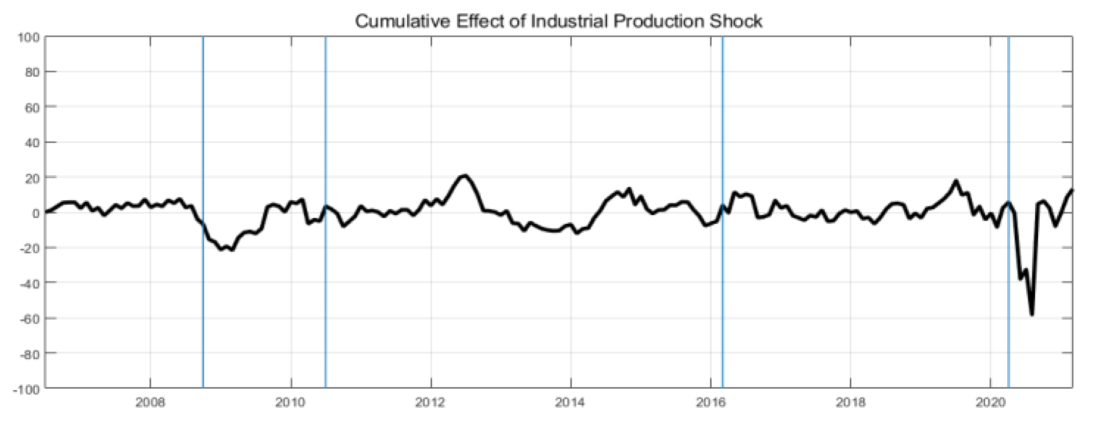
According to the historical decomposition of Korea’s ocean-going maritime transport revenue, the increase in maritime transportation revenue until 2008 was largely affected by the increase in the BDI, whereas the decline in freight rates in 2009 was attributed to a decrease in the BDI due to the drop in OECD industrial production and world trade volume (Figure 3). Subsequently, the increase and decrease in the BDI mainly caused the fluctuations; during the COVID-19 period, there was a downward impact from the rapid industrial production paralysis and a decrease in the world trade volume, as was the case during the global financial crisis. However, the speed of recovery was faster than that after the global financial crisis.

The historical decomposition of the volume of new shipbuilding contracts worldwide demonstrated that, as in the shipping industry model, the increase in new shipbuilding contracts until 2008 was driven by the increase in the BDI (Figure 4). Thereafter, the volume of new shipbuilding contracts worldwide seems to have decreased due to the decline in industrial production caused by the global financial crisis and the resulting decrease in the world trade volume and freight rates. During 2014, the decrease in the world trade volume, in line with the sharp drop in oil prices caused by the increase in shale oil production in the US, can be interpreted as having affected the volume of new shipbuilding contracts. In addition, the volume of new shipbuilding contracts was greatly affected by the BDI in 2016, when the BDI hit a record low. During the COVID-19 period, as with the shipping industry model, it was immediately affected by the decline in OECD industrial production and world trade volume, but with a faster recovery.

3.4. Local Projection Estimation Results

The robustness of the results was checked by using the impulse response functions from the LP model. The results from the LP model show similar patterns as those from the SVAR model.

Figure 5 presents the impulse response functions of maritime transport revenue and the volume of new shipbuilding contracts for shipping and macroeconomic shocks, at the 90% confidence interval. The left panel of Figure 5 is the impulse response function of maritime transport revenue, and the right panel shows the impulse response function of the volume of new shipbuilding contracts.

The effects of the volume of new shipbuilding contracts worldwide on macroeconomic variable shocks are as follows. First, the BDI shock is found to increase the volume of new shipbuilding contracts for a short period, but its effect gradually dissipates. The industrial production index shock increases the volume of new shipbuilding contracts in the short run, but the effect dissipates after decline and fluctuations. Unexpected changes in the world trade volume index increase the volume of new shipbuilding contracts, but their statistical significance is low.

According to the above analysis, unexpected shocks to the shipping and macroeconomic variables variously appear in maritime transport revenue and new shipbuilding contracts, but cumulatively, they positively affect all the variables.

These results are consistent with the Granger causality test and SVAR estimation results analyzed earlier. Thus, the results from this study explain the cycle of the classic maritime supply-demand model [20], in which global economic demand affects shipping freight rates; these, in turn, affect new ships orders and the revenue of shipping companies, directly affecting shipping companies’ investment decisions.

4. Conclusions

This study examined the dynamic effects of macroeconomic shocks on the shipping industry (shipping account in the balance of payments) and shipbuilding industry (volume of new shipbuilding contracts worldwide). This analysis has the following implications. According to the Granger causality analysis, OECD industrial production, the world trade volume index, and the BDI, all Granger-cause maritime transport revenue. Furthermore, the OECD industrial production and world trade volume indices and the BDI Granger-cause the volume of new shipbuilding contracts worldwide. According to the impulse response analyses of the recursive SVAR and LP models, shocks from the industrial production index, world trade volume index, and BDI increase maritime transport revenue and new shipbuilding contracts. The results suggest that unexpected increases in macroeconomic and shipping variables have a positive impact on the performance of shipping and shipbuilding industries.

In the shipping industry, the causes of their effects were empirically identified for each period and the differences in the responses by period were analyzed in the historical decomposition analysis. As such, the dynamic relationship between the shipping industry and shipbuilding industry is presented by the existing theoretical model and previous research, according to which the macroeconomy as well as shipping and shipbuilding industries are sequentially affected.

The contributions of this study are as follows. It provides a quantitative analysis of how macroeconomic variables affect shipping industry performance (shipping account in the balance of payments) in a country and new shipbuilding contracts in the shipbuilding industry. By examining the effects of macroeconomic changes on the shipbuilding and shipping industries, this study is expected to provide the players in those industries with useful information for interpreting macroeconomic variables in terms of corporate operations and investment strategies.

In addition, policymakers can utilize the information arising from the relevance of related industries in their strategies to further enhance shipping industry performance. In particular, such information would be useful for developing policies in countries such as Korea where both the shipping and the shipbuilding industries are present.

However, the major macroeconomic variables, apart from the variables presented in this study, affecting the shipping and shipbuilding industries will need to be examined, to determine the direction and extent of their effects. An international comparison of the effects in each country would also provide useful information.

In summary, the dynamic relationship between the macroeconomic variables and shipping and shipbuilding industry variables should be noted, since their correlation can be used in decision-making, especially for corporate operations and policy development in the industry.

Meanwhile, the recursive structure used to identify shocks in this study is a strong identifying restriction, even though the order of variables is set based on generally accepted economic theory. Thus, to address this limitation, future studies can conduct analyses using the SVAR model that identifies shocks through sign restrictions. Furthermore, as shown in the analytical results of this study, since the shipping market is closely related to the global economy, further studies will be needed to classify the period of global economic crisis and analyze the response of the shipping market for each economic crisis.

References

- UNCTAD. Review of Maritime Transport 2020; United Nations Conference on Trade and Development: Geneva, Switzerland, 2021; p. 20. [Google Scholar] [CrossRef]
- Michail, N.A.; Melas, K.D. Quantifying the relationship between seaborne trade and shipping freight rates: A Bayesian vector autoregressive approach. Marit. Transp. Res. 2020, 1, 100001. [Google Scholar] [CrossRef]
- Isserlis, L. Tramp shipping cargoes, and freights. J. R. Stat. Soc. 1938, 101, 53–146. [Google Scholar] [CrossRef]
- Hawdon, D. Tanker freight rates in the short and long run. Appl. Econ. 1978, 10, 203–218. [Google Scholar] [CrossRef]
- Strandenes, S.P. Price determination in the time charter and second-hand markets. In Center for Applied Research, Norwegian School of Economics and Business Administration Discussion Paper No. 5; Norwegian School of Economics and Business Administration: Bergen, Norway, 1984; pp. 1–47. [Google Scholar]
- Beenstock, M.; Vergottis, A. An econometric model of the world tanker market. J. Transp. Econ. Policy 1989, 23, 263–280. Available online: https://www.jstor.org/stable/20052891 (accessed on 9 October 2021).
- Beenstock, M.; Vergottis, A. Econometric Modelling of World Shipping; Chapman & Hall: London, UK, 1993. [Google Scholar]
- Kavussanos, M.G.; Marcoulis, S.N. The stock market perception of industry risk and macroeconomic factors: The case of the US water and other transportation stocks. Int. J. Marit. Econ. 2000, 2, 235–256. [Google Scholar] [CrossRef]
- Grammenos, C.T.; Arkoulis, A.G. Macroeconomic factors and international shipping stock returns. Int. J. Marit. Econ. 2002, 4, 81–99. [Google Scholar] [CrossRef]
- Kilian, L. Not all oil price shocks are alike: Disentangling demand and supply shocks in the crude oil market. Am. Econ. Rev. 2009, 99, 1053–1069. [Google Scholar] [CrossRef] [Green Version]
- Klovland, J.T. Business Cycles, Commodity Prices and Shipping Freight Rates: Some Evidence from the Pre-WWI Period. Workshop on Market Performance and the Welfare Gains of Market Integration in History. SNF. 2002. Available online: https://openaccess.nhh.no/nhh-xmlui/bitstream/handle/11250/165223/R48_02.pdf?sequence=1 (accessed on 9 October 2021).
- Michail, N.A. World economic growth and seaborne trade volume: Quantifying the relationship. Transp. Res. Interdiscip. Perspect. 2020, 4, 100108. [Google Scholar] [CrossRef]
- Papapostolou, N.C.; Nomikos, N.K.; Pouliasis, P.K.; Kyriakou, I. Investor sentiment for real assets: The case of dry bulk shipping market. Rev. Financ. 2014, 18, 1507–1539. [Google Scholar] [CrossRef]
- Kogan, L.; Livdan, D.; Yaron, A. Oil Futures Prices in a Production Economy with Investment Constraints. J. Financ. 2009, 64, 1345–1375. [Google Scholar] [CrossRef]
- Gavriilidis, K.; Kambouroudis, D.S.; Tsakou, K.; Tsouknidis, D.A. Volatility forecasting across tanker freight rates: The role of oil price shocks. Transp. Res. E 2018, 118, 376–391. [Google Scholar] [CrossRef] [Green Version]
- Lim, K.G.; Nomikos, N.K.; Yap, N. Understanding the fundamentals of freight markets volatility. Transp. Res. E 2019, 130, 1–15. [Google Scholar] [CrossRef]
- Drobetz, W.; Schilling, D.; Tegtmeier, L. Common risk factors in the returns of shipping stocks. Marit. Policy Manag. 2010, 37, 93–120. [Google Scholar] [CrossRef]
- Tsouknidis, D.A. Dynamic volatility spillovers across shipping freight markets. Transp. Res. E 2016, 91, 90–111. [Google Scholar] [CrossRef]
- Syriopoulos, T.; Roumpis, E. Dynamic correlations and volatility effects in the Balkan equity markets. J. Int. Financ. Mark. Inst. Money 2009, 19, 565–587. [Google Scholar] [CrossRef]
- Stopford, M. Maritime Economics, 3rd ed.; Routledge: New York, NY, USA, 2009. [Google Scholar]
- Kou, Y.; Luo, M. Modelling the relationship between ship price and freight rate with structural changes. J. Transp. Econ. Policy 2015, 49, 276–294. [Google Scholar]
- Alizadeh, A.H.; Nomikos, N.K. Investment timing and trading strategies in the sale and purchase market for ships. Transp. Res. B Methodol. 2007, 41, 126–143. [Google Scholar] [CrossRef]
- Veenstra, A.W. Quantitative Analysis of Shipping Market; Delft University Press: Amsterdam, The Netherlands, 1999. [Google Scholar]
- Xu, J.J.; Leung, Y.T.; Liming, L. Dynamic interrelationships between sea freight and shipbuilding markets. In Proceedings of the International Forum on Shipping, Ports and Airports (IFSPA 2008)—Trade-Based Global Supply Chain and Transport Logistics Hubs: Trends and Future Development, Hong Kong, China, 25–28 May 2008; pp. 480–494. [Google Scholar]
- Jiang, L.; Lauridsen, J.T. Price formation of dry bulk carriers in the Chinese shipbuilding industry. Marit. Policy Manag. 2012, 39, 339–351. [Google Scholar] [CrossRef] [Green Version]
- Xu, J.J.; Yip, T.L. Ship investment at a Standstill? An Analysis of Shipbuilding Activities and Policies. Appl. Econ. Lett. 2012, 19, 269–275. [Google Scholar] [CrossRef] [Green Version]
- Yin, J.; Luo, M.; Fan, L. Dynamics and interactions between spot and forward freights in the dry bulk shipping market. Marit. Policy Manag. 2017, 44, 271–288. [Google Scholar] [CrossRef]
- Jiang, B.; Li, J.; Gong, C. Maritime shipping and export trade on “Maritime Silk Road”. Asian J. Ship. Logist. 2018, 34, 83–90. [Google Scholar] [CrossRef]
- Chen, Z.; Zhang, X.; Chai, J. The dynamic impacts of the global shipping market under the background of oil price fluctuations and emergencies. Complexity 2021, 2021, 1–13. [Google Scholar]
- Gu, Y.; Dong, X.; Chen, Z. The relation between the international and China shipping markets. Res. Transp. Bus. Manag. 2020, 34, 100427. [Google Scholar] [CrossRef]
- Granger, C.W.J. Investigating causal relations by econometric models and cross-spectral methods. Econometrica 1969, 37, 424–438. [Google Scholar] [CrossRef]
- Lütkepohl, H. New Introduction to Multiple Time Series Analysis; Springer Science & Business Media: Berlin/Heidelberg, Germany, 2005. [Google Scholar]
- Kilian, L.; Lütkepohl, H. Structural Vector Autoregressive Analysis; Cambridge University Press: Cambridge, UK, 2017. [Google Scholar] [CrossRef] [Green Version]
- Sims, C.S. Money, income, and causality. Am. Econ. Rev. 1972, 62, 540–552. [Google Scholar]
- Chamberlain, G. The general equivalence of Granger and Sims causality. Econometrica 1982, 50, 569–581. [Google Scholar] [CrossRef]
- Geweke, J. Inference and causality in econometric time series models. In Handbook of Econometrics; Griliches, Z., Intriligator, M., Eds.; Elsevier Science Publishers: Amsterdam, The Netherlands, 1984; Volume 2, pp. 1101–1144. [Google Scholar]
- Diebold, F.X. Elements of Forecasting; South-Western College Pub.: Cincinnati, OH, USA, 1998. [Google Scholar]
- Kim, T.-I.; Yoon, J.-W.; Park, S.-H. Analysis of and Response Measures to Ship Investment Behaviors of Shipping Companies; Korea Maritime Institute: Busan, Korea, 2017. [Google Scholar]
- Klein, L.R. Economic Fluctuations in the United States, 1921–1941; John Wiley: New York, NY, USA, 1950. [Google Scholar]
- Klein, L.R.; Goldberger, A.S. An Econometric Model of the United States; North Holland Publishing Company: Amsterdam, The Netherlands, 1955. [Google Scholar]
- Tinbergen, J. The Dynamics of Share-Price Formation. Rev. Econ. Stat. 1939, 21, 153–160. [Google Scholar] [CrossRef] [Green Version]
- Sims, C.A. Macroeconomics and reality. Econometrica 1980, 48, 1–48. [Google Scholar] [CrossRef] [Green Version]
- Kilian, L. Structural Vector Autoregressions. In Handbook of Research Methods and Applications in Empirical Macroeconomics; CEPR Discussion Papers; Edward Elgar Publishing: Cheltenham, UK, 2011. [Google Scholar]
- Cooley, T.F.; Dwyer, M. Business cycle analysis without much theory A look at structural VARs. J. Econ. 1998, 83, 57–88. [Google Scholar] [CrossRef]
- Sims, C. Are forecasting models usable for policy analysis? Fed. Reserve Bank Minneap. Q. Rev. 1986, 10, 2–16. [Google Scholar] [CrossRef]
- Bernanke, B.S. Alternative explanations of the money-income correlation. Carnegie Rochester Conf. S. Public Policy 1986, 25, 49–99. [Google Scholar] [CrossRef] [Green Version]
- Blanchard, O.J.; Watson, M.W. Are business cycles all alike? In The American Business Cycle: Continuity and Change; Gordon, R., Ed.; University of Chicago Press: Chicago, IL, USA, 1986; pp. 123–156. [Google Scholar]
- Park, S.-H. A Study on Business Fluctuation and Risk Assessment in the Shipping Market. Ph.D. Thesis, Pusan National University, Busan, Korea, 2019. [Google Scholar]
- Shapiro, M.D.; Watson, M.W. Sources of business cycle fluctuations. In NBER Macroeconomics Annual; Stanley, F., Ed.; MIT Press: Cambridge, MA, USA, 1988; Volume 3, pp. 111–148. [Google Scholar] [CrossRef]
- Blanchard, O.J.; Quah, D. The dynamic effects of aggregate demand and aggregate supply disturbances. Am. Econ. Rev. 1989, 79, 655–673. [Google Scholar]
- Keating, J. Structural approaches to vector autoregressions. Fed. Reserve Bank St. Louis Rev. 1992, 74, 37–57. [Google Scholar] [CrossRef] [Green Version]
- Faust, J. The robustness of the identified VAR conclusions about money. Carnegie Rochester Conf. S. Public Policy 1998, 49, 207–244. [Google Scholar] [CrossRef] [Green Version]
- Canova, F.; Pina, J.P. Monetary policy misspecification in VAR models. Center for Economic Policy Research Discussion Paper. SSRN J. 1999. [Google Scholar] [CrossRef] [Green Version]
- Canova, F.; Nicoló, G.D. Monetary disturbances matter for business fluctuations in the G-7. J. Monet. Econ. 2002, 49, 1131–1159. [Google Scholar] [CrossRef] [Green Version]
- Uhlig, H. What are the effects of monetary policy on output? Results from an agnostic identification procedure. J. Monet. Econ. 2005, 52, 381–419. [Google Scholar] [CrossRef] [Green Version]
- Kim, K.-H.; Yoon, S.-H. Asymmetry and nonlinearity analysis of the effects of oil prices and exchange rates on consumer prices. Int. Econ. Res. 2009, 15, 131–152. [Google Scholar]
- Jordà, Ò. Estimation and inference of impulse responses by local projections. Am. Econ. Rev. 2005, 95, 161–182. [Google Scholar] [CrossRef]
- Ramey, V.A. Macroeconomic shocks and their propagation. In Handbook of Macroeconomics; Taylor, J.B., Uhlig, H., Eds.; Elsevier: Amsterdam, The Netherlands, 2016; Volume 2, pp. 71–162. [Google Scholar]
- Newey, W.K.; West, K.D. Automatic lag selection in covariance matrix estimation. Rev. Econ. Stud. 1994, 61, 631–653. [Google Scholar] [CrossRef]
- Ebregt, J. The CPB World Trade Monitor: Technical Description; CPB Background Document; The CPB Netherlands Bureau for Economic Policy Analysis: The Hague, The Netherlands, 2016.
- Hodrick, R.; Prescott, E.C. Post-War US Business Cycles: An Empirical Investigation. Discussion Paper 451; Northwestern University, Center for Mathematical Studies in Economics and Management Science: Evanston, IL, USA, 1980. [Google Scholar]
- Población, J.; Serna, G. A Common Long-Term Trend for Bulk Shipping Prices. Marit. Econ. Logist. 2018, 20, 421–432. [Google Scholar] [CrossRef]
- Bai, X.; Lam, J.S.L. An Integrated Analysis of Interrelationships within the Very Large Gas Carrier (VLGC) Shipping Market. Marit. Econ. Logist. 2019, 21, 372–389. [Google Scholar] [CrossRef]
- Gonçalves, S.; Kilian, L. Bootstrapping autoregressions with conditional heteroskedasticity of unknown form. J. Econom. 2004, 123, 89–120. [Google Scholar] [CrossRef] [Green Version]
Figure 1.
Responses of maritime transport revenue to shocks from the major variables. Note: the x-axis represents the time lag (months) and the y-axis values are percentages.
Figure 2.
Responses of the volume of new shipbuilding contracts to shocks from the major variables. Note: the x-axis represents the time lag (months) and the y-axis values are percentages.
Figure 3.
Historical decomposition results of the shipping industry model. Note: the y-axis values are percentage deviations from the mean.
Figure 4.
Historical decomposition results of the shipbuilding industry model. Note: the y-axis values are percentage deviations from the mean.
Figure 5.
Over 10 months, followed by a return to the original level, the industrial production index shock significantly increases Korea’s ocean-going maritime transport revenue. Meanwhile, the world trade volume index shock increases Korea’s maritime transport revenue for about eight months, but its effect dissipates after repeated fluctuations.