Prevention of Mountain Disasters and Maintenance of Residential Area through Real-Time Terrain Rendering

Abstract

Climate change increases the frequency of localized heavy rains and typhoons. As a result, mountain disasters, such as landslides and earthworks, continue to occur, causing damage to roads and residential areas downstream. Moreover, large-scale civil engineering works, including dam construction, cause rapid changes in the terrain, which harm the stability of residential areas. Disasters, such as landslides and earthenware, occur extensively, and there are limitations in the field of investigation; thus, there are many studies being conducted to model terrain geometrically and to observe changes in terrain according to external factors. However, conventional topography methods are expressed in a way that can only be interpreted by people with specialized knowledge. Therefore, there is a lack of consideration for three-dimensional visualization that helps non-experts understand. We need a way to express changes in terrain in real time and to make it intuitive for non-experts to understand. In conventional height-based terrain modeling and simulation, there is a problem in which some of the sampled data are irregularly distorted and do not show the exact terrain shape. The proposed method utilizes a hierarchical vertex cohesion map to correct inaccurately modeled terrain caused by uniform height sampling, and to compensate for geometric errors using Hausdorff distances, while not considering only the elevation difference of the terrain. The mesh reconstruction, which triangulates the three-vertex placed at each location and makes it the smallest unit of 3D model data, can be done at high speed on graphics processing units (GPUs). Our experiments confirm that it is possible to express changes in terrain accurately and quickly compared with existing methods. These functions can improve the sustainability of residential spaces by predicting the damage caused by mountainous disasters or civil engineering works around the city and make it easy for non-experts to understand.

1. Introduction

Owing to global warming and environmental pollution, phenomena related to climate change, such as landslides, are causing massive damage to residential areas [1]. Countries with mountainous terrain, such as China, suffer a lot of damage from mountain disasters. According to data collected by The Fatal Landslide Event Inventory of China (FLEIC) from 1950 to 2016, there were 1911 landslides and 28,139 deaths in China [2]. The total number of fatal landslides recorded worldwide, excluding those triggered by earthquakes, over the 12 calendar years between 2004 and 2016 (inclusive) was 4862 [3]. The whole world is working to prevent such natural disasters in advance. Identifying changes in terrain is one of the important research topics to prevent disasters, such as landslides, in advance. A number of studies have been proposed to analyze the mechanisms of landslides, such as “stage-wise” methodologies utilizing geo-hydro-mechanical (GHM) [4]. The effects of weathering or sedimentation over a long period of time cannot be ignored, but large-scale civil engineering or dam construction in a particular area can also have a significant impact on the surrounding terrain in the short term [5]. Previously, experts in the environment and terrain used paper maps, numerical maps, and aerial photographs to estimate changes in the terrain [6]. With the recent prevalence of light direction and ranging (LiDAR), which measures the position coordinates of reflectors by shooting laser pulses and measuring the return time, high resolution terrain data can be obtained [7]. Furthermore, recently, it has been possible to obtain high-resolution data and images at a relatively low price using unmanned aerial vehicles (UAVs) [8] or photogrammetry using drones. UAVs are also utilized for data collection in hazardous areas such as volcanoes [9]. However, the source of such acquired information cannot be visualized and shown intuitively, and it also requires professional knowledge to be interpreted.

In addition, most of these studies only deal with photographs taken periodically or non-periodically to look at changes in the terrain that have occurred over a relatively short period of time, making it difficult to predict possible changes in terrain in the future. Because all terrain is interconnected, local changes in terrain affect a wide range of regions, and 3D-based real-time terrain simulations are required to efficiently represent them [10]. Converting sampled terrain data to three-dimensional geometric information not only makes it easy to calculate variations, but also allows for visualization with high resolution images, and allows non-experts to intuitively observe and interpret terrain changes. In addition to mountain disasters, real-time terrain modeling and rendering technology are preferred over professional data analysis tools because the opinions of experts in urban planning and civil engineering should be well explained to the general public, who do not have expertise in the area.

Three-dimensional real-time rendering technology is being used in various fields beyond simply copying the virtual world in movies and games [11]. One of these fields is simulation; when presenting environmental phenomena or objects using computing tools, state-of-the-art computer graphics techniques are indispensable for more realistic and accurate analysis [12].

A data elevation model (DEM) is used to represent the terrain as an alternative, as scanning terrain and rendering the same data with reality is still impossible even in modern computer graphics devices. A DEM is a set of ground surface height values obtained from uniformly sampled spaces, typically measured using 3D scanning techniques [13]. With higher quality and improved resolution of the measured data, better graphics processing units (GPUs) and memory are required to render terrain based on DEM data in real time. Many algorithms using GPUs are being studied to render large-scale geographic data using a single graphics accelerator [14,15].

Typical methods include the quadtree technique proposed by Lindstrom [16] and the real-time optimally adaptive meshes (ROAM) technique using the binary tree structure proposed by Duchaineau [17]. Lindstrom used a bottom-up approach to determine the segmentation and merging of the quadtree. ROAM uses a binary tree structure that dynamically generates terrain over time. Each patch is a simple isostatic triangle with a structure in which each triangle is recursively divided into two child nodes. This method is called screen error. In this method, based on the error between real terrain and its estimated model, the terrain that is higher than the error set by the user recursively divides. The detailed level of the terrain below the error is adjusted in such a way that no segmentation is made. In the level-of-detail (LOD) methods [18,19], a multi-resolution grid based on the distance between the camera and the object is used in the out-of-core terrain visualization algorithm.

Recent topographic rendering techniques use GPUs to perform mesh reconstruction by swapping limited geometric information such as vertex relocation [20] and persistent grid mapping (PGM) [21]. These techniques reduce errors by randomly swapping a certain number of regular grids. Because the amount of geometry data remains unchanged, these methods have the advantage of constant rendering speed, simpler operation, and being faster than conventional mesh reconstruction methods. However, because mesh cannot be optimized based on error, many geometric errors occur, showing results that are different from the real terrain. To address these topographical rendering problems, we extract the roughness of the terrain based on a regular lattice map and determine that the part with a specific threshold or higher roughness is a curved terrain. A vertex of the 3D mesh can be gathered in a curved terrain rather than in a fixed interval to represent a more accurate terrain than a regular grid map. We propose a method for efficient LOD by managing vertex relocated cohesion maps in a hierarchical structure. This differs from conventional regular grid-based methods [22,23] by measuring geometric errors in Hausdorff distances for the accuracy of twisted terrain. This geometric error value is measured in chunks and the LOD is determined based on this chunk to render the terrain. To improve the efficiency of error computation, we use the Hausdorff distance instead of an existing regular grid that considers only the height differences in the terrain.

For accurate terrain rendering, it is necessary to determine the rendering criteria of the LOD considering geometric errors. The Hausdorff distance is an algorithm for calculating distance, which is a method of calculating the upper and lower bounds for the distances of two sets and any element to which they belong. We apply an approximation of the Hausdorff distance, which holds the upper bound on the distance of the surface normal as a criterion for terrain error by comparing the two vertex groups in which triangulation is generated [24]. This method can be operated faster than other circular mesh-based methods, such as batched dynamic adaptive meshes (BDAM) [25,26,27], and can be effectively used in map applications with frequent topographical modifications and updates.

To make an accurate comparison of the geometric error, we compare the plane of the existing height-field-based terrain rendering to our proposed method. Based on the results, we experimented with Chunk LOD and the proposed method to render and compare the valleys. By selecting a specific point of representation and measuring geometric errors, our method rendered much more accurate and sophisticated data than the GPU-based Chunk LOD. Our method solves the geometric error problem arising from the existing warping-based vertex cohesion map and expresses a more realistic terrain.

Section 2 discusses existing research techniques used to visualize terrain data, Section 3 details methods for the vertex cohesion map and the Hausdorff distance, Section 4 shows the results compared to the existing Chunk LOD method, and Section 5 concludes.

2. Related Works

A fractal is characterized by its self-similarity, so the shape of the part resembles the whole. Based on this feature, successful results in modeling natural phenomena have been obtained through a midpoint segmentation algorithm using random fractal [28] and a diamond/square algorithm [29], a branch of fractal geometry invented by Mandelbrot in the mid-1970s. Using the characteristics of random fractals, these algorithms are used to model virtual terrain and are very useful for generating various forms of realistic terrain [30], but it is very difficult to predict the final form of terrain created by randomness. Even if we want to model a terrain that is close to reality, it is difficult to predict the shape of the terrain until the result is printed on the screen. We try to solve this problem by proposing a terrain modeling algorithm that limits the Gaussian distribution function utilized in generating the terrain data so that it does not deviate from a predefined outer surface or pyramid structure [31]. However, there was a problem with complex forms of terrain modeling that required too many control points to work unless it was simple terrain modeling.

DEM data obtain high and low values of the surface by photographing the terrain through aerial measurement equipment (LiDAR) or satellites. Unlike other model data storage methods, the DEM data are in an image format. The size of the image becomes the size of the actual measured terrain, and the color value that the pixel has indicates the actual height of the actual terrain. Using image-type storage methods has the advantage of having visual convenience, providing easy management and modification, and modeling realistic forms of terrain. The higher the resolution, the higher the computation for the area within the uniform sample interval, which results in a longer processing time required. In traditional central processing unit (CPU)-based approaches, the number of triangles was adjusted using hierarchical structures such as triangular binary trees [16] or restricted quadtrees [32], which were efficient in eliminating regions or out-of-sight triangles that did not require segmentation. Triangular binary tree methods can store more geometry data [23] than quadtree methods. The Chunk LOD [33] reduces the computation required to select LODs by using a geometric cache in the form of a specific area geometry chunk.

Since the introduction of programmable GPU pipelines, GPU-based rendering techniques such as geometry image warping [34] have been introduced. The vertex cohesion map simplifies the mesh by extracting key features mainly from the DEM data, using elasticity [35] between the vertices of the terrain mesh. As a result, a GPU can be used to reconstruct and render terrain faster than a CPU. However, owing to the limitations of available memory space, out of core algorithms are widely used [36,37]. An important problem with core extrinsic-based algorithms is to reduce the transmission time to transfer data to the GPU memory. To address this problem, GPU-based geometry decompression techniques [38] using decompressed data in GPUs are proposed, as this is how to use image layers, such as geometry clipmaps [18]. Researchers attempt to speed-up triangular rasterization and improve efficiency with fast and straightforward simplification techniques rather than simplifying the terrain using continuous development of the GPUs [14,39]. These approaches have the advantage of being able to scale out of core and can perform fast rendering by leveraging parallel processing of GPUs, but there are many drawbacks to data considering memory efficiency and terrain roughness, as they typically only perform distance-based LODs.

3. Real-Time Terrain Simulation Using a Vertex Cohesion Map

Terrain modeling and rendering using a vertex cohesion map is faster and more accurate than the existing terrain mesh reconstruction methods. However, it cannot provide LOD generation and selection based on accurate screen error. The proposed method uses the Hausdorff distance [24] to solve this problem. The Hausdorff distance refers to the maximum distance difference between the original data and the modified data. Therefore, when the terrain data of a specific area are transformed into a vertex cohesion map, the maximum geometric error with the original data can be accurately derived. Using the Hausdorff distance as a geometric error matrix, a vertex cohesion map can be applied to the conventional methods that performed the LOD selection using geometric errors.

Figure 1 shows the procedure of the proposed method, which is co-processed in the CPU and the GPU [40,41]. The geometric error of the reconstructed terrain chunk is calculated using the GPU in the preprocessing step. We create a quadtree, a representative data structure used in the terrain LOD, so that the LOD technique can be applied to the area based on the geometric error of the chunk.

3.1. Processing Step of the Vertex Cohesion Map

A simplified regular terrain mesh represents the terrain by the displacement of the vertex from the height field data. The surface roughness is proportional to the frequency of geometric errors. Usually, surface roughness is estimated using a Laplacian operator. However, when using the Laplacian operator, a small bump may have a greater amount of roughness than a mountain.

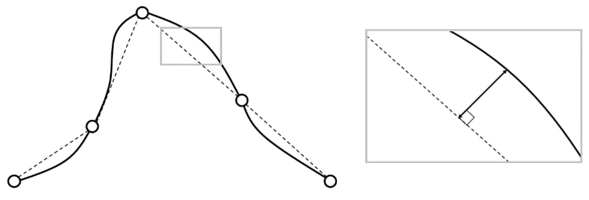
Figure 2 shows an example of an incorrect estimation of the surface roughness, which is a good example in this case. When estimating the surface roughness at each position of the gray vertex, because θ_a is smaller than θ_b, the terrain in (a) may have greater surface roughness than that in (b). However, the geometric error δ_b is bigger than δ_a. To estimate the roughness more accurately, we apply Gaussian smoothing, which is a well-known method for noise reduction [42]. Gaussian smoothing efficiently solves the Laplacian operator problem for bumps with the distance-based weight. Through the convolution of the Gaussian smoothing prior to the Laplacian, we can obtain laplacian of gaussian (LoG) as follows.

LoG(x,y) = −1/πσ⁴[1 − (x² + y²/2σ²)e^{−(x2+y2)/2σ2}

(1)

Figure 3 shows how the terrain is reconstructed using a vertex cohesion map. The vertex coherence vector is stored in the vertex coherence map. This vector moves the vertices to locations where a large Hausdorff distance appears. Peaks and valleys will be the representative example. These points can occur through geometric popping (geo-popping).

The cohesion vector in the vertex cohesion data is determined as a summation of the cohesion vector, which is related to elastic forces between vertices. The elastic force causes the vertices to push or pull each other when they are closer or farther than their initial distance. The following equation describes Hooke’s law of elasticity. This equation is a commonly used approximation for elastic forces:

F_e = −k * (l’ − l)

(2)

where l is the initial length of the spring between vertices [43], l’ is the length of the spring of a deformed terrain mesh, and k is the modulus of elasticity. Our previous work [18] modified this algorithm using the elastic force between the centroid and the vertex, as shown in Figure 4. Vertices A, B, C, D, and P are relocated vertices of regular grids and T is the centroid of □ABCD.

We use a centroid for the ideal position that balances the weight of the terrain patch. Finding the centroid T of an N-polygon can be expressed as follows:

T_x = ∑^N−1(x_i + y_i) (x_iy_i+1 − x_i+1y_i)/6S

(3)

T_y =∑^N−1(y_i + x_i) (y_ix_i+1 − y_i+1x_i)/6S

(4)

where S is the area of the N-polygon. We used Heron’s formula to compute the area S. We assume that the elastic force pulls a central vertex P toward the centroid of the quadrilateral □ABCD, as shown in Figure 5. Thus, the vector in our method V_e is formulated as

V_e = K’P’T

(5)

where K is the adaptive modus of the elasticity in Equation (5). It is very difficult to determine a reasonable way to fix the value of K. When K is too small, the cohesion vector will be too large and geometrical overlapping or twisting may occur. On the other hand, a large value of K will intensify the elastic force. This might hold vertices and disturb the deformation. Therefore, we define K, which is proportional to the difference in area between the original regular grid and the deformed grid, as below.

If   a < τ_low or a > τ_up, then k = 1,

(6)

else if   τ_low ≤ a < 1, then k = (1 − a)/(1 − τ_low),

(7)

else if   1 ≤ a ≤ τ_up, then k = a/τ_up

(8)

where a is the ratio of regular quads (input data) to □ABCD. In addition, τ_low and τ_up are user-defined threshold values. When the area of □ABCD becomes either larger or smaller, the elastic force between T and P becomes stronger. Therefore, a strong elastic force will pull P toward the centroid when the neighboring vertices are too deformed. Otherwise, the elastic force will be weak, and P will be affected more by the cohesion forces.

In order to balance these forces, the proposed method uses a resolution ratio between the vertex cohesion map and the original terrain data. In general, the height field, which is the original data, is measured more accurately as the resolution increases. However, in the case of the vertex cohesion map, the original data are reduced with multiresolution. Therefore, this ratio varies for each detail level. For example, in the case of a 1/4-sized vertex cohesion map, the ratio is reduced 1/2 times horizontally and vertically. Therefore, when calculating the maximum movement of the vertex, it is appropriate to set τ_low to 1/2 and τ_up to 2. In the case of 1/64, 64 is 2⁸, so it is appropriate to set τ_low to 1/8 and τ_up to 8. The larger the area is reduced, the larger the movement of the vertex is set. Therefore, the proposed method creates a vertex cohesion map by setting τ differently for each resolution. Therefore, as in the following equation, we finally compute the cohesion vector V through a summation of the attraction and elastic forces as follows:

V = V_e + ∑A_n

(9)

As shown in Figure 5, the proposed method performs the LOD of the terrain models using the Hausdorff distance, which measures the maximum distance from the surface normal to the original data. In general, the terrain can be managed by subdividing the area into a quadtree. In this area, the depth of the quadtree is configured for each detail level of the vertex coherence map. Each node stores how much Hausdorff distance it has at the detail level so that the maximum error value can be calculated in screen space.

3.2. Terrain Reconstruction Using Hierarchical Vertex Cohesion Map

In this section, we explain how to efficiently use the GPU and the CPU at the same time to improve rendering speed. In general, the quadtree reconstructs the terrain by a GPU-based tree traversal algorithm. However, when the rendering process is distributed by dividing it into several renders passes, there is a task of the CPU unit that creates a GPU command to draw for each chunk and a task of the GPU that executes the command. Each task can be processed simultaneously. In general, in 3D applications, the GPU works asynchronously, so the CPU searches the quadtree. At this time, the appropriate detail level of the vertex cohesion map is selected so that the corresponding data can be rendered on the GPU. The larger the data, the more a bottleneck occurs in the quadtree traversal of the CPU. Therefore, when there are many operations to be processed, a separate GPU pass is designed so that operations being parallelized in the GPU can be performed through the compute shader [44].

The vertex cohesion map does not reduce geometric errors significantly, even at a more detailed level. Sometimes, there is also a case where the geometric error increases. In this case, in the proposed method, the geometric error may be smaller in the case of rendering with a rougher vertex cohesion map than in the case where it is not. Therefore, if you need to use a child node whose geometric error is larger than that of the parent node in the quadtree, the accuracy of the terrain may be degraded. In this case, the vertex cohesion map stored in the parent node is used. This makes it possible to show an optimal rendering speed in an image that guarantees the same error. If the detail level of the adjacent terrain is different, cracks on the terrain appear due to the T-vertex. Therefore, it is necessary to know the detail level of the neighbor node. This difference in detail level matches the detail level of the neighboring node in the chunk and prepares a pass for creating a patch so that cracks can be removed.

The CPU always stores information about the commands to be drawn in the quadtree parser. The quadtree parser is a list that stores the nodes of the quadtree where the index for the vertex cohesion map that generated the current command is stored. This list allows you to fill commands into the command buffer immediately when there is no camera movement. In addition, as the LOD selection can be performed directly from the node information selected in the previous frame without having to search the quadtree from the root node, the amount of computation can be greatly reduced. This optimization is very important because the CPU’s pre-LOD selection task needs to be processed faster than the rendering LOD.

4. Discussion and Experimental Results

We measured the number of frames per second of the conventional method (the Chunk LOD method) and then compared it to the proposed method to prove the efficiency of the proposed method. For the cohesion vector calculation, it took an average of 0.34 s to generate a terrain with a resolution of 64² using the GPU (total eight detail level).

All experiments were performed on a consumer PC equipped with and Intel Core^TM i5 3.3 GHz CPU, 16 GB of main memory. The GPU is nVidia^TM GeForce GTX 1060 graphic card with 3 GB of local graphic memory. We used the DirectX 11 and the shader model 5.0 as the graphics API. We used the 16-bit Jeju Island, Puget Sound and the Grand Canyon dataset, which are well-known benchmarking data. As the limitation of the texture size of the graphic hardware is 8192 × 8192, we set the resolution of the vertex cohesion map as 64 × 64. The viewport size was set to 1920 × 1080 pixels.

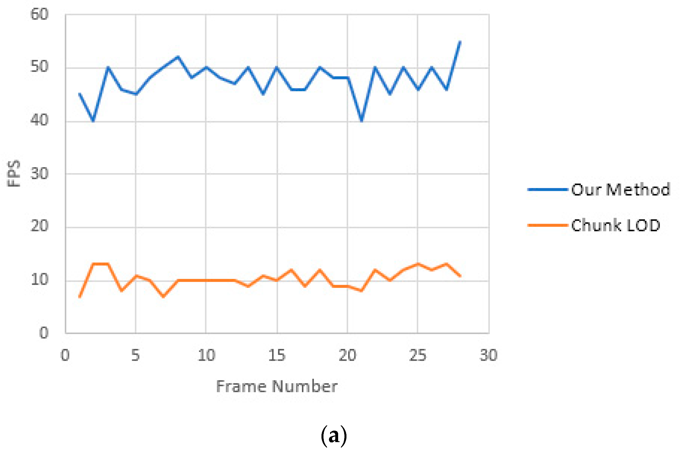
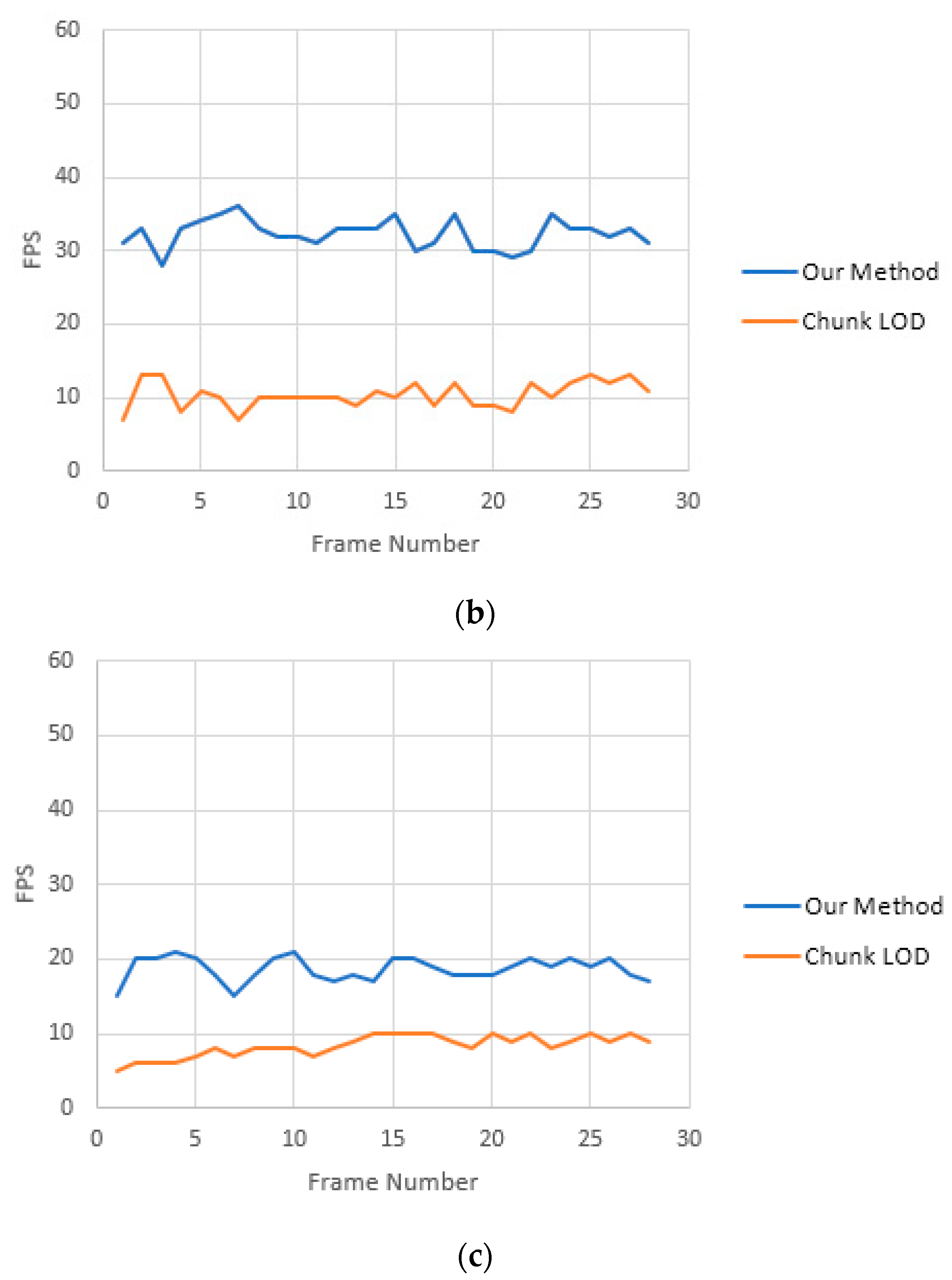
Figure 6 shows a comparison of the rendering speed between the proposed method and the GPU-based Chunk LOD while using the same chunk size. We set the Hausdorff distance to two pixels as the threshold value for selecting the detail level. This is because it takes more than one second to render a frame using the conventional method when the current measurement condition is attached to the ground at a maximum of one pixel or less. When the error tolerance is set to two pixels, it is easy to compare fps, as 5 fps is guaranteed in the conventional method, as shown in Figure 7. Our method showed that the average rendering speed becomes 298.3% of the previous method. The average fastest speed is 358% of the classical method in the Puget Sound, which consists of a lot of flat land, and the slowest average is 224% in the Grand Canyon, which contains several complex valleys. This figure shows that it can render the data three times faster on average than it takes in real time using a usual amount of computation. Therefore, it is possible to render high-resolution terrain data in real time using existing terrain measurement equipment, which is difficult to render in real time.

Figure 7 is the measurement result of memory consumption. The method proposed in the figure saved memory of up to 79% and an average of 71%. This can effectively reduce the cost of communication with the server. For example, in a work environment with poor network conditions, even if the network is slow, the number of downloads is small, so you can achieve the advantage of speed improvement.

In the proposed method, rendering speed is important. Therefore, by generating high-resolution data and giving distortion, terrain data of 100 m per pixel were created. Based on these data, the accuracy of the vertex cohesion map was measured. Figure 8 shows the main valley data from the Puget Sound. The red dots are the main locations of the selected valleys. Acceleration is meaningful only when there are no errors at these key points.

In

Table 1. Maximum error and number of errors of the proposed method.

	Max Geometric Error	Number of Errors (Bigger than 100 m)	Number of Errors (Bigger than 50 m)
Puget Sound	136 m (1.36 pixel)	2	4
Jeju Island	143 m (1.43 pixel)	1	3
Grand Canyon	157 m (1.57 pixel)	1	4

and

Table 2. Maximum error and number of errors of the conventional method.

	Max Geometric Error	Number of Errors (Bigger than 100 m)	Number of Errors (Bigger than 50 m)
Puget Sound	175 m (1.75 pixel)	5	7
Jeju Island	192 m (1.92 pixel)	2	5
Grand Canyon	183 m (1.83 pixel)	3	9

, in order to measure the accuracy of the proposed method, geometric errors were measured by selecting specific points representing valleys on the map. The number of errors (red dots) measured are shown in Figure 8. The pixel error was measured in the final image rendered at a specific camera point. Compared with the experimental result comparison method (the GPU-based Chunk LOD), it shows much more accurate and sophisticated data. This reduces false operations based on simplified data for real-time rendering. Therefore, with the proposed method, the work can be performed more elaborately and quickly in the existing work environment. However, there is the disadvantage that it takes about 0.3 s to produce each chunk. Furthermore, it is efficient because it can extract at about three times the rendering speed and about two times more accurately with a pre-processing process in less than one second.

5. Conclusions

This paper presents an efficient GPU-based terrain modeling and rendering technique that can increase the efficiency of the LOD selection and eliminate geometric errors. Existing terrain simulation approaches based on the height-field focus primarily on how large amounts of terrain are being reconstructed at a high speed. By warping a regular grid sample, it can improve performance by reducing errors in rendering compared with conventional mesh reconstruction. However, the resulting warping results in geometric error, resulting in the reconstruction of the mesh with different forms from the real terrain surface. To solve this problem, our method stores how much Hausdorff distance is at the corresponding detail level to allow calculation of the maximum error values in screen space. The Hausdorff distance can solve the geometric error problem arising from the existing warping-based vertex cohesion map. Furthermore, the processing of vertex cohesion maps and the geometry error was pre-processed at the GPU level, which allowed us to identify that the sample topography is faster than the existing height-field based papers. Our method renders a more accurate terrain by solving the geometric error held by the existing regular grid-based terrain rendering. It can be useful in terms of residential maintenance because it is possible to predict the damage caused by mountainous disasters around a city by checking changes in the terrain in real time.