
Development of Simplified Building Energy Prediction Model to Support Policymaking in South Korea—Case Study for Office Buildings

 ,
,
Abstract
:1. Introduction
2. Methodology
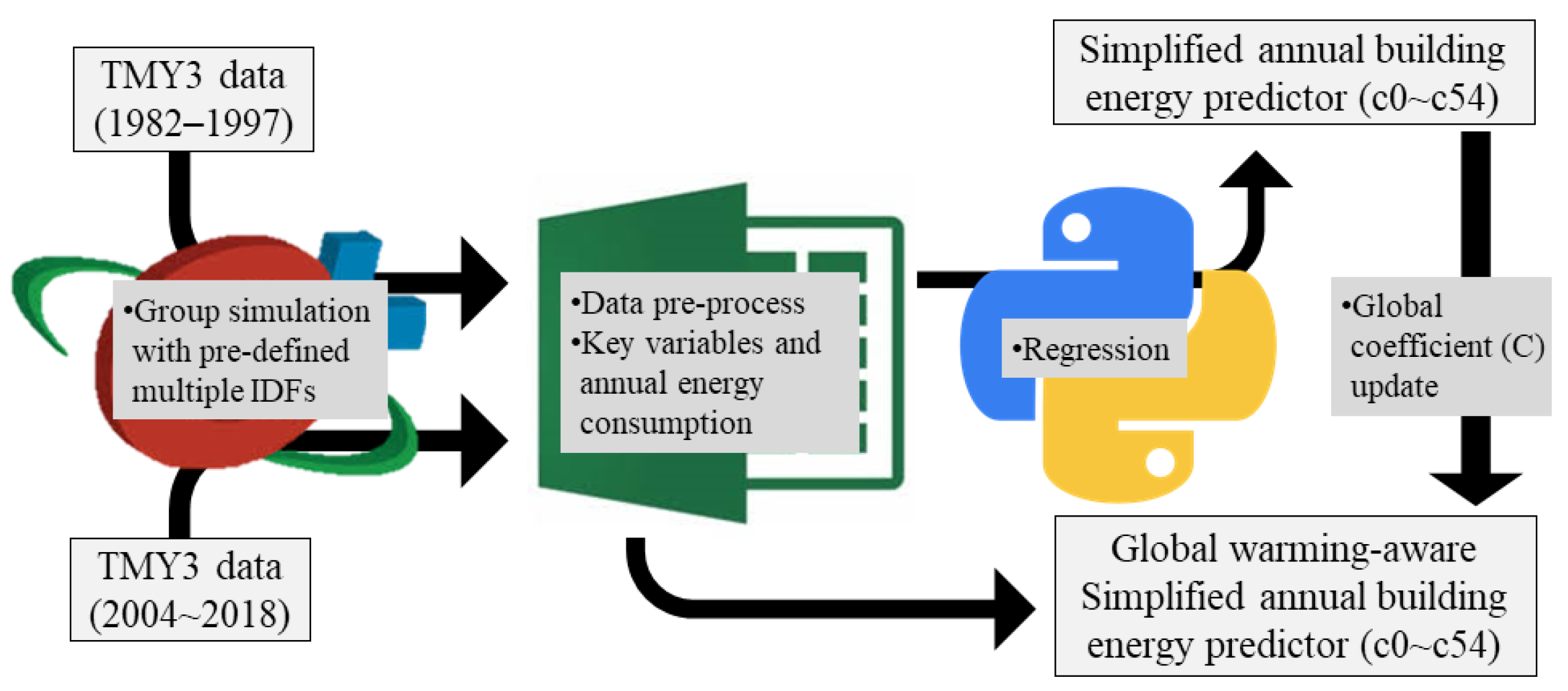
2.1. Research Flow
2.2. Reference Building Models
- Residential: Lowvilla, House, Apartment (APT)
- Commercial: Retail, Restaurant, Hotel, Private office, Hospital
- Public: Public office, School, University
2.3. Weather Profile
2.4. Key Variables for Model Inputs
2.5. Model Structure and Regression Method
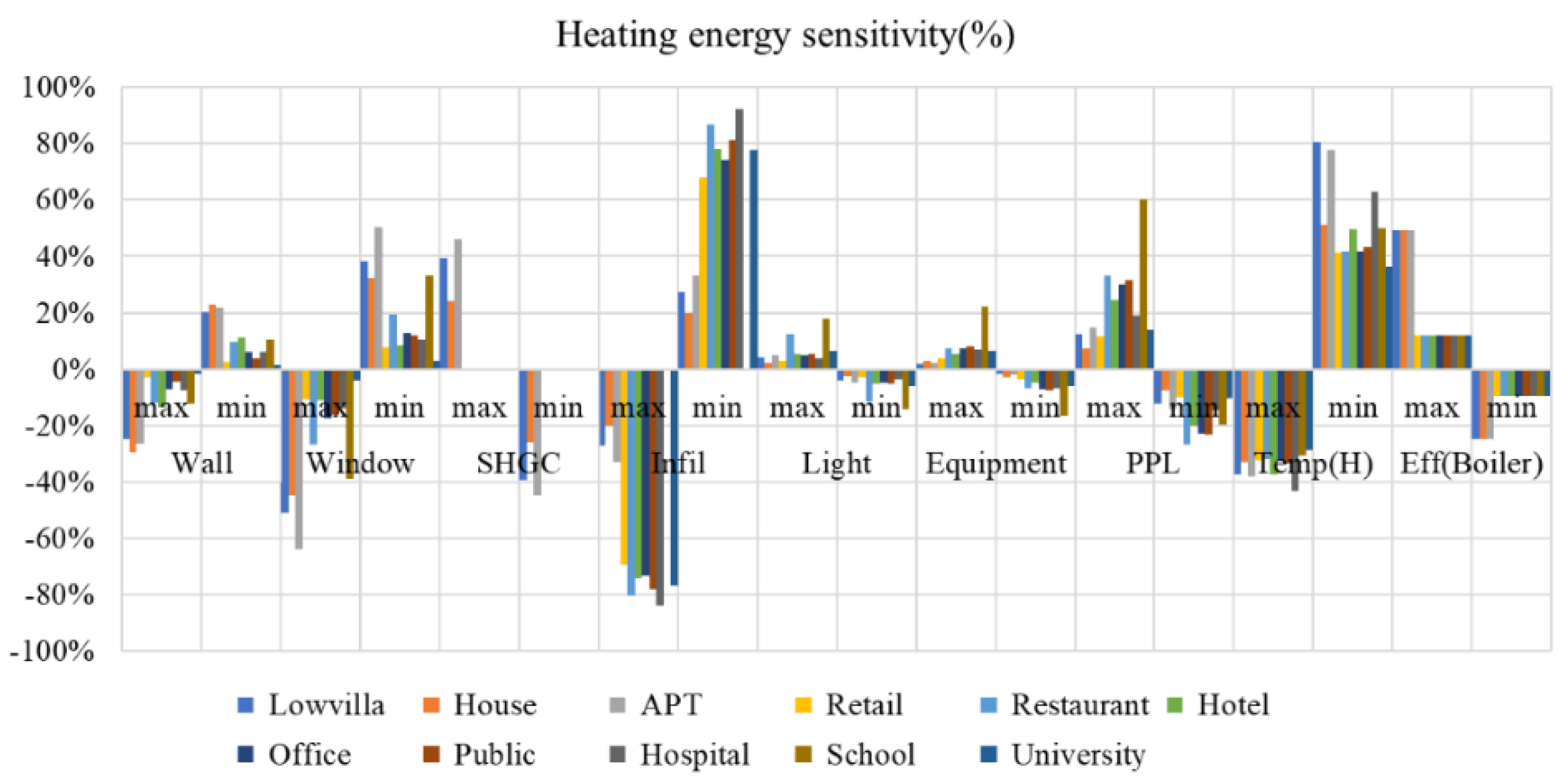
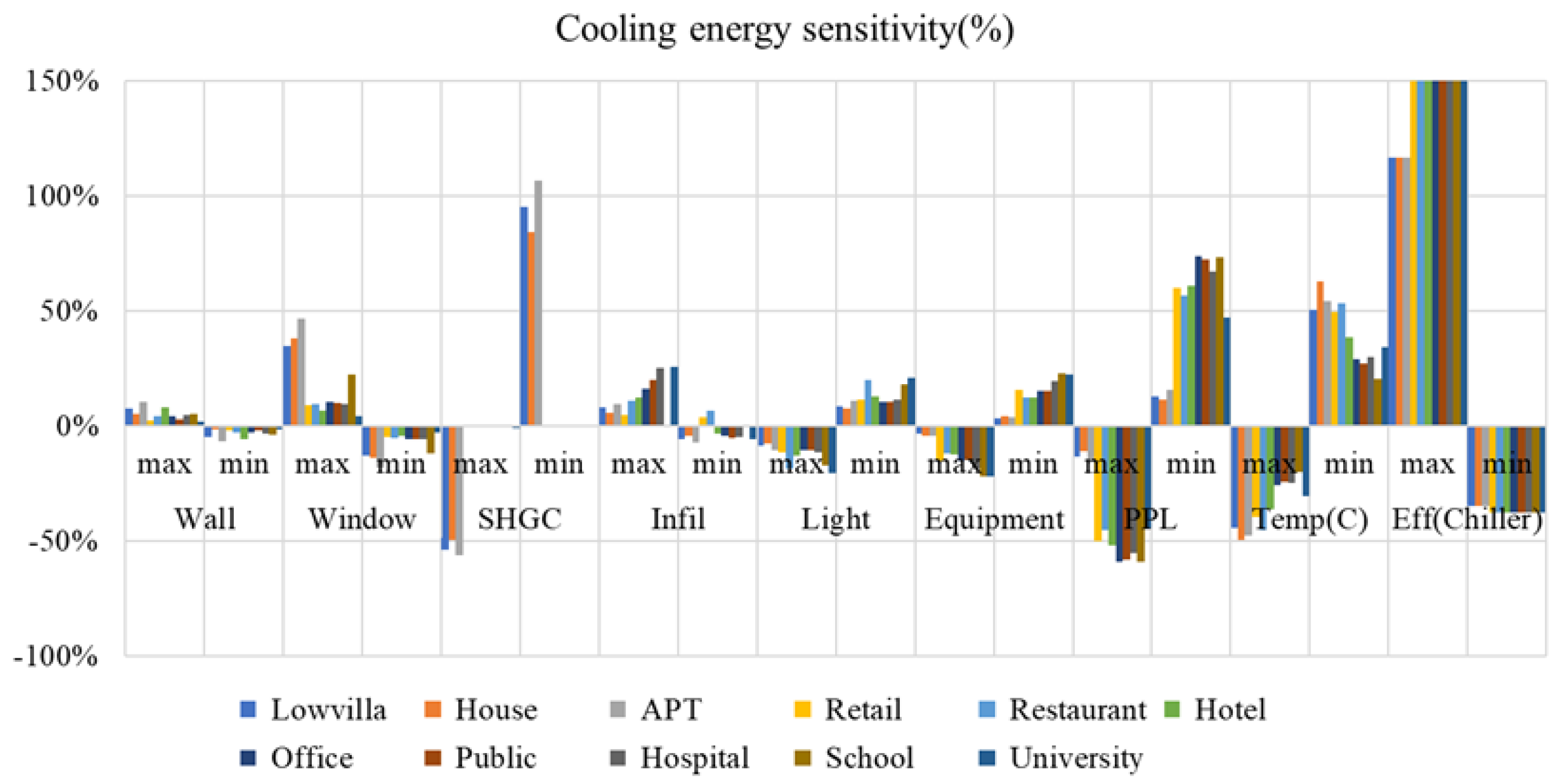
3. Preliminary Results with Reference Buildings
Regression Results and Sensitivity
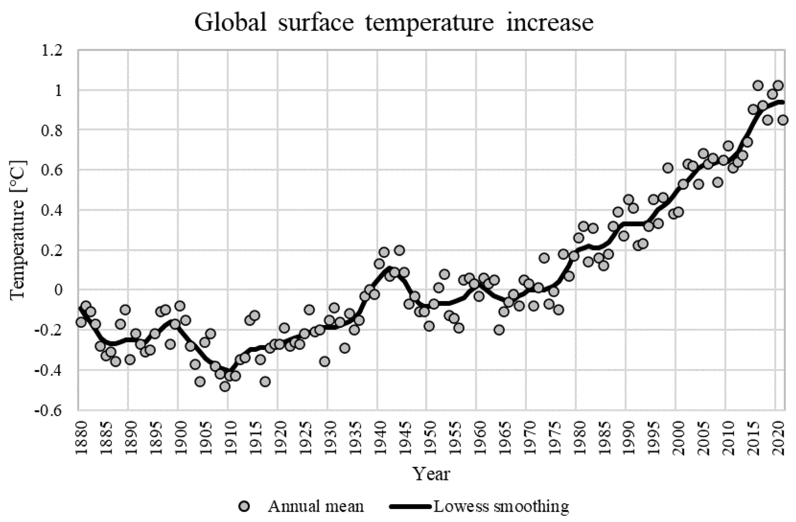
4. Multivariate Model Evaluation with Office Building in a Global Warming Scenario
5. Conclusions
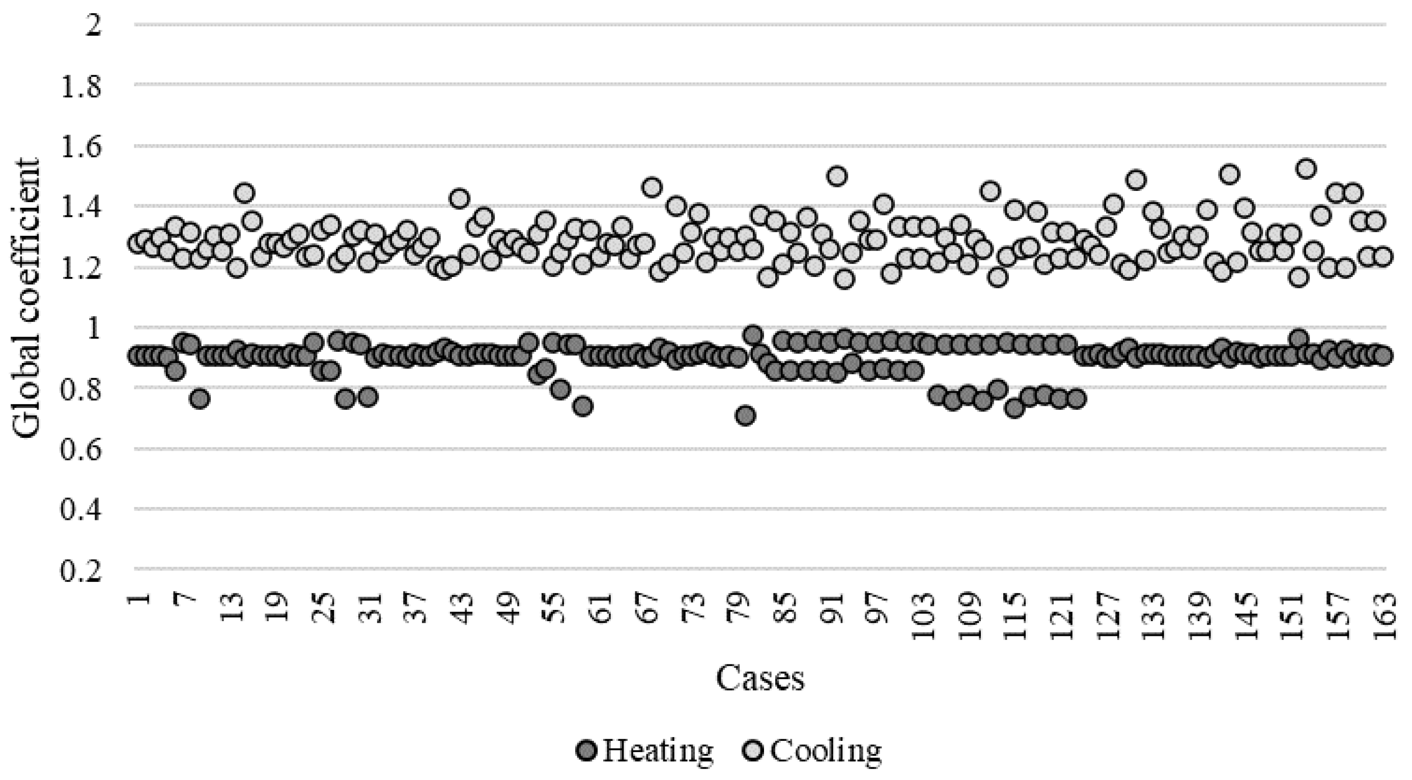
- The global coefficients considering global warming with increased outdoor air temperatures were estimated to be 1.27 and 0.9 for cooling and heating, respectively; this means 27% more and 10% less energy consumption in 20 years, according to predictions.
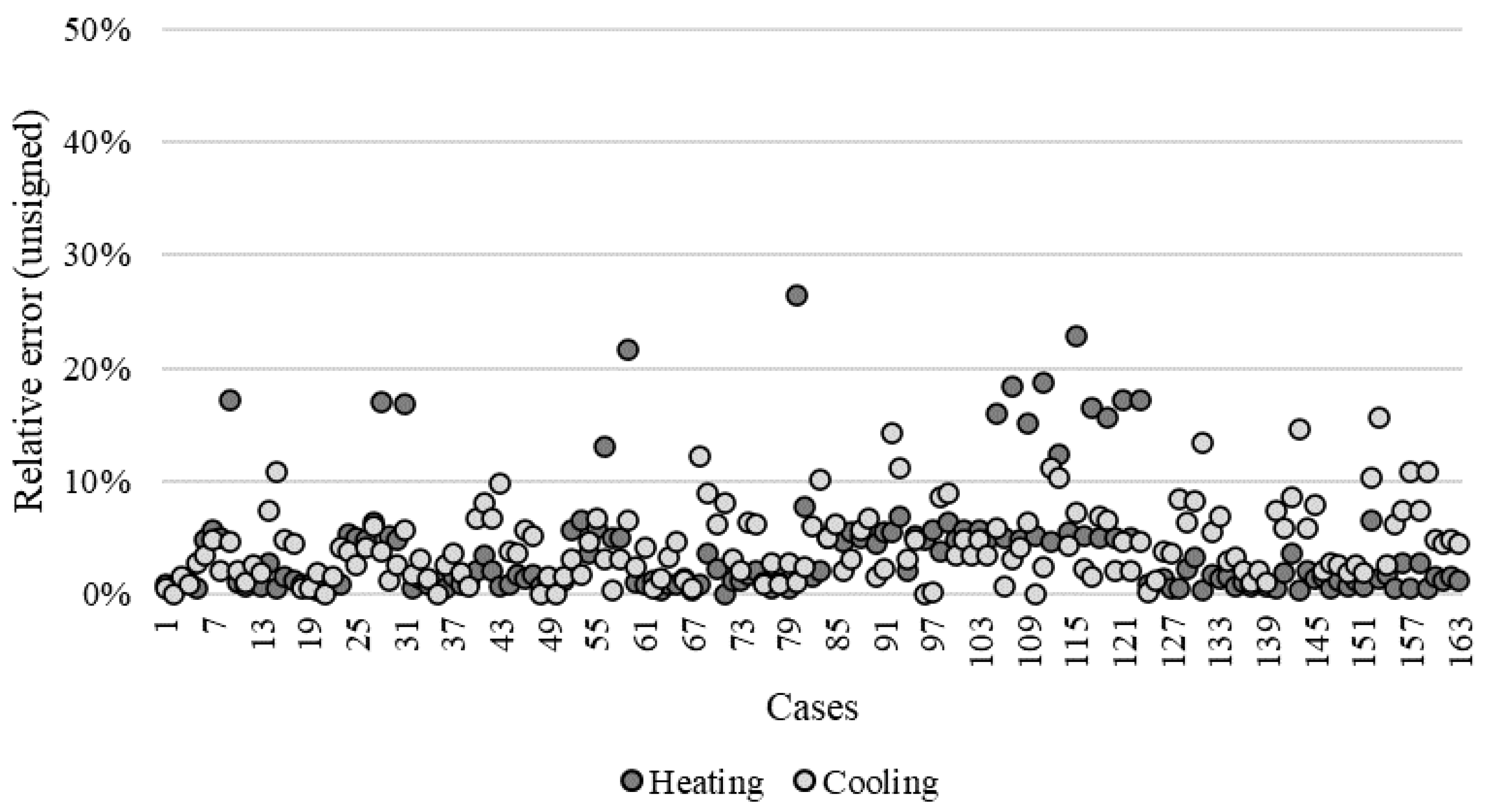
- The prediction performance of the simplified regression model (163 cases) was generally good, with cvRMSE values of 4.3% and 5.5%, while the maximum absolute errors were 26% and 16% for the heating and cooling cases, respectively.
6. Discussion
Author Contributions
Funding
Institutional Review Board Statement
Informed Consent Statement
Data Availability Statement
Conflicts of Interest
Appendix A

| Min | Med | Max | ||
|---|---|---|---|---|
| Insulation | Envelope | 0.08 | 0.59 | 1.1 |
| Windows | 0.5 | 2.25 | 4 | |
| SHGC | 0.2 | 0.525 | 0.85 | |
| Infiltration | 0.2 | 0.39 | 0.58 | |
| Internal heat gains | Lighting | 2 | 8.5 | 15 |
| Equipment | 1.5 | 4.75 | 8 | |
| People | 0.01 | 0.04 | 0.07 | |
| Setpoint temperatures | Heating | 17 | 20.5 | 24 |
| Cooling | 29 | 27 | 25 | |
| HVAC efficiencies | Heating | 0.5 | 0.745 | 0.99 |
| Cooling | 1.5 | 3.25 | 5 | |
| Min | Med | Max | |||
|---|---|---|---|---|---|
| Insulation | Envelope | 0.1 | 0.55 | 1 | |
| Windows | 0.5 | 2.25 | 4 | ||
| SHGC | 0.2 | 0.5 | 0.8 | ||
| Infiltration | 0.3 | 1.15 | 2 | Otherwise | |
| 0.3 | 1.65 | 3 | Restaurant | ||
| 0.3 | 0.9 | 1.5 | Hotel | ||
| 0.2 | 1.1 | 2 | Hospital | ||
| Internal heat gains | Lighting | 2 | 8 | 14 | |
| Equipment | 2 | 8 | 14 | ||
| People | 0.2 | 0.6 | 1 | Otherwise | |
| 0.2 | 0.5 | 0.8 | Hotel | ||
| Setpoint temperatures | Heating | 18 | 20.5 | 23 | Otherwise |
| 18 | 21 | 24 | Restaurant, Hotel | ||
| 18 | 22 | 26 | Hospital | ||
| Cooling | 28 | 26 | 24 | Otherwise | |
| 28 | 25.5 | 23 | Restaurant, Hotel | ||
| HVAC efficiencies | Heating | 0.8 | 0.895 | 0.99 | |
| Cooling | 1 | 2.5 | 4 | ||
| Min | Med | Max | ||
|---|---|---|---|---|
| Insulation | Envelope | 0.1 | 0.55 | 1 |
| Windows | 0.5 | 2.25 | 4 | |
| SHGC | 0.2 | 0.5 | 0.8 | |
| Infiltration | 0.3 | 1.15 | 2 | |
| Internal heat gains | Lighting | 2 | 8 | 14 |
| Equipment | 2 | 8 | 14 | |
| People | 0.2 | 0.6 | 1 | |
| Setpoint temperatures | Heating | 18 | 20.5 | 23 |
| Cooling | 28 | 26 | 24 | |
| HVAC efficiencies | Heating | 0.8 | 0.895 | 0.99 |
| Cooling | 1 | 2.5 | 4 | |
References
- Carfí, D.; Donato, A.; Schiliró, D. Competitive solutions of environmental agreements for the global economy after COP21 in Paris. J. Environ. Manag. 2019, 249, 109331. [Google Scholar] [CrossRef] [PubMed]
- Ali, K.A.; Ahmad, M.I.; Yusup, Y. Issues, impacts, and mitigations of carbon dioxide emissions in the building sector. Sustainability 2020, 12, 7427. [Google Scholar] [CrossRef]
- Galvin, R.; Healy, N. The Green New Deal in the United States: What it is and how to pay for it. Energy Res. Soc. Sci. 2020, 67, 101529. [Google Scholar] [CrossRef]
- Lee, J.H.; Woo, J. Green new deal policy of south Korea: Policy innovation for a sustainability transition. Sustainability 2020, 12, 10191. [Google Scholar] [CrossRef]
- IEA (International Energy Agency). Global Energy-Related CO2 Emissions by Sector. 2021. Available online: https://www.iea.org/data-and-statistics/charts/global-energy-related-co2-emissions-by-sector (accessed on 15 March 2022).
- Economidou, M.; Todeschi, V.; Bertoldi, P.; D’Agostino, D.; Zangheri, P.; Castellazzi, L. Review of 50 years of EU energy efficiency policies for buildings. Energy Build. 2020, 225, 110322. [Google Scholar] [CrossRef]
- He, Q.; Hossain, M.U.; Ng, S.T.; Augenbroe, G. Identifying practical sustainable retrofit measures for existing high-rise residential buildings in various climate zones through an integrated energy-cost model. Renew. Sustain. Energy Rev. 2021, 151, 111578. [Google Scholar] [CrossRef]
- He, C.; Hou, Y.; Ding, L.; Li, P. Visualized literature review on sustainable building renovation. J. Build. Eng. 2021, 44, 102622. [Google Scholar] [CrossRef]
- IIbañez Iralde, N.S.; Pascual, J.; Salom, J. Energy retrofit of residential building clusters. A literature review of crossover recommended measures, policies instruments and allocated funds in Spain. Energy Build. 2021, 252, 111409. [Google Scholar] [CrossRef]
- Li, Y.; O’Neill, Z.; Zhang, L.; Chen, J.; Im, P.; DeGraw, J. Grey-box modeling and application for building energy simulations—A critical review. Renew. Sustain. Energy Rev. 2021, 146, 111174. [Google Scholar] [CrossRef]
- Ljung, L. System Identification. In Theory for the User, 2nd ed.; Prentice Hall PTR: Upper Saddle River, NJ, USA, 1999. [Google Scholar]
- Lu, C.; Li, S.; Lu, Z. Building energy prediction using artificial neural networks: A literature survey. Energy Build. 2022, 262, 111718. [Google Scholar] [CrossRef]
- Chen, S.; Zhou, X.; Zhou, G.; Fan, C.; Ding, P.; Chen, Q. An online physical-based multiple linear regression model for building’s hourly cooling load prediction. Energy Build. 2022, 254, 111574. [Google Scholar] [CrossRef]
- Li, X.; Wang, C.; Kassem, M.A.; Wu, S.-Y.; Wei, T.-B. Case study on carbon footprint life-cycle assessment for construction delivery stage in China. Sustainability 2022, 14, 5180. [Google Scholar] [CrossRef]
- Deru, M.; Field, K.; Studer, D.; Benne, K.; Griffith, B.; Torcellini, P.; Liu, B.; Halverson, M.; Winiarski, D.; Rosenberg, M.; et al. U.S. Department of Energy Commercial Reference Building Models of the National Building Stock; National Renewable Energy Laboratory: Golden, CO, USA, 2011; pp. 1–118. Available online: http://digitalscholarship.unlv.edu/renew_pubs/44 (accessed on 15 March 2022).
- The European Parliament and the Council of the European Union. Directive 2010/31/EU of the European parliament and of council of 19 May 2010 on the energy performance of buildings (recast). Off. J. Eur. Union. 2010, 18, 153. Available online: https://eur-lex.europa.eu/legal-content/EN/TXT/PDF/?uri=CELEX:32010L0031&rid=4 (accessed on 15 March 2022).
- Kwak, Y.; Kang, J.; Mun, S.H.; Jeong, Y.S.; Huh, J.H. Development and application of a flexible modeling approach to reference buildings for energy analysis. Energies 2020, 13, 5815. [Google Scholar] [CrossRef]
- Kwak, Y.; Kang, J.A.; Huh, J.H.; Kim, T.H.; Jeong, Y.S. An analysis of the effectiveness of greenhouse gas reduction policy for office building design in South Korea. Sustainability 2019, 11, 7172. [Google Scholar] [CrossRef] [Green Version]
- Ye, Y.; Hinkelman, K.; Zhang, J.; Zuo, W.; Wang, G. A methodology to create prototypical building energy models for existing buildings: A case study on U.S. religious worship buildings. Energy Build. 2019, 194, 351–365. [Google Scholar] [CrossRef]
- de Vasconcelos, A.B.; Pinheiro, M.D.; Manso, A.; Cabaço, A. EPBD cost-optimal methodology: Application to the thermal rehabilitation of the building envelope of a Portuguese residential reference building. Energy Build. 2016, 111, 12–25. [Google Scholar] [CrossRef]
- Buso, T.; Corgnati, S.P. A customized modelling approach for multi-functional buildings—Application to an Italian Reference Hotel. Appl. Energy 2017, 190, 1302–1315. [Google Scholar] [CrossRef]
- Yang, X.; Liu, S.; Zou, Y.; Ji, W.; Zhang, Q.; Ahmed, A.; Han, X.; Shen, Y.; Zhang, S. Energy-saving potential prediction models for large-scale building: A state-of-the-art review. Renew. Sustain. Energy Rev. 2022, 156, 111992. [Google Scholar] [CrossRef]
- Campagna, L.M.; Fiorito, F. On the Impact of Climate Change on Building Energy Consumptions: A Meta-Analysis. Energies 2022, 15, 354. [Google Scholar] [CrossRef]
- Kim, D.W.; Kim, Y.M.; Lee, S.H.; Park, W.Y.; Bok, Y.J.; Ha, S.K.; Lee, S.E. Development of Reference Building Energy Models for South Korea. In Proceedings of the 15th IBPSA Conference, San Francisco, CA, USA, 7–9 August 2017. [Google Scholar]
- Crawley, D.B.; Lawrie, L.K.; Winkelmann, F.C.; Buhl, W.F.; Huang, Y.J.; Pedersen, C.O.; Strand, R.K.; Liesen, R.J.; Fisher, D.E.; Witte, M.J.; et al. EnergyPlus: Creating a new-generation building energy simulation program. Energy Build. 2001, 33, 319–331. [Google Scholar] [CrossRef]
- Byrd, R.H.; Lu, P.; Nocedal, J.; Zhu, C. A limited memory algorithm for bound constrained optimization. SIAM J. Sci. Comput. 1995, 16, 1190–1208. [Google Scholar] [CrossRef]
- Wilcox, S.; Marion, W. Users Manual for TMY3 Data Sets S. Technical Report NREL/TP-581-43156 Revised May 2008. Available online: https://www.nrel.gov/docs/fy08osti/43156.pdf (accessed on 15 March 2022).
- Kim, J.-H.; Lim, H.-W.; Lee, H.-S.; Shin, U.-C. Shin Review on the Effectiveness of Apartments According to Insulation Reinforcement of Energy Saving Design Standard. J. Archit. Inst. Korea Struct. Constr. 2020, 36, 173–178. [Google Scholar]
- Kim, J.-H.; Sung, J.-E.; Kim, H.-G.; Park, D.-J.; Kim, S.-S. Improvement in Energy Performance of Office Buildings according to the Evolution of Building Energy Code. J. KIAEBS 2020, 14, 101–111. [Google Scholar]
- Global Temperature, Global Land-Ocean Temperature Index. Available online: https://data.giss.nasa.gov/gistemp/graphs/graph_data/Global_Mean_Estimates_based_on_Land_and_Ocean_Data/graph.txt (accessed on 15 March 2022).


Publisher’s Note: MDPI stays neutral with regard to jurisdictional claims in published maps and institutional affiliations. |
© 2022 by the authors. Licensee MDPI, Basel, Switzerland. This article is an open access article distributed under the terms and conditions of the Creative Commons Attribution (CC BY) license (https://creativecommons.org/licenses/by/4.0/).
Share and Cite
Joe, J.; Min, S.; Oh, S.; Jung, B.; Kim, Y.M.; Kim, D.W.; Lee, S.E.; Yi, D.H. Development of Simplified Building Energy Prediction Model to Support Policymaking in South Korea—Case Study for Office Buildings. Sustainability 2022, 14, 6000. https://doi.org/10.3390/su14106000
Joe J, Min S, Oh S, Jung B, Kim YM, Kim DW, Lee SE, Yi DH. Development of Simplified Building Energy Prediction Model to Support Policymaking in South Korea—Case Study for Office Buildings. Sustainability. 2022; 14(10):6000. https://doi.org/10.3390/su14106000
Chicago/Turabian StyleJoe, Jaewan, Seunghyeon Min, Seunghwan Oh, Byungwoo Jung, Yu Min Kim, Deuk Woo Kim, Seung Eon Lee, and Dong Hyuk Yi. 2022. "Development of Simplified Building Energy Prediction Model to Support Policymaking in South Korea—Case Study for Office Buildings" Sustainability 14, no. 10: 6000. https://doi.org/10.3390/su14106000
APA StyleJoe, J., Min, S., Oh, S., Jung, B., Kim, Y. M., Kim, D. W., Lee, S. E., & Yi, D. H. (2022). Development of Simplified Building Energy Prediction Model to Support Policymaking in South Korea—Case Study for Office Buildings. Sustainability, 14(10), 6000. https://doi.org/10.3390/su14106000