Study-GNN: A Novel Pipeline for Student Performance Prediction Based on Multi-Topology Graph Neural Networks

Abstract

Student performance prediction has attracted increasing attention in the field of educational data mining, or more broadly, intelligent education or “AI + education”. Accurate performance prediction plays a significant role in solving the problem of a student dropping out, promoting personalized learning and improving teaching efficiency, etc. Traditional student performance prediction methods usually ignore the potential (underlying) relationship among students. In this paper, we use graph structure to reflect the students’ relationships and propose a novel pipeline for student performance prediction based on newly-developed multi-topology graph neural networks (termed MTGNN). In particular, we propose various ways for graph construction based on similarity learning using different distance metrics. Based on the multiple graphs of different topologies, we design an MTGNN module, as a key module in the pipeline, to deal with the semi-supervised node classification problem where each node represents a student (and the node label is the student’s performance, e.g., Pass/Fail/Withdrawal). An attention-based method is developed to produce the unified graph representation in MTGNN. The effectiveness of the proposed pipeline is verified in a case study, where a real-world educational dataset and several existing approaches are used for performance comparison. The experiment results show that, compared with some traditional machine learning methods and the vanilla graph convolutional network with only a single graph topology, our proposed pipeline works effectively and favorably in student performance prediction.

1. Introduction

With the rise and development of online education, learning management systems (LMS) are widely used in distance education institutions. A large amount of diversified learning data are generated and recorded, which provides valuable data for learning analytics. Learning analytics is a process to evaluate students’ academic performance, predicting their learning performance and finding problems through the analysis and interpretation of the relevant data generated and collected by learners. It covers the collection, measurement, analysis, reporting and knowledge discovery of data about students, teachers and institutions [1]. According to the 2021 EDUCAUSE Horizon Report, the foundational data of learning analysis includes course-level data, such as evaluation scores collected from the LMS and institutional-level data residing in student information systems, registration records, financial systems and institutional research units [2]. Educational big data is profoundly affecting and changing education. How to make full use of educational data and explore the educational law behind it has become the focus of researchers in recent years. The main task of learning analysis in the field of education is to analyze and interpret the relevant data generated and collected by learners, evaluate the learner’s academic performance, predict their academic performance, and carry out academic early warning according to the prediction results of learning status to provide a basis for educational decision-making. Therefore, making full use of educational data to predict learners’ academic performance is not only the core issue in the field of learning analysis, it is also a research hotspot in the field of education. Student performance prediction aims to estimate the future performance of students in a specific examination or evaluation. This helps identify whether students are at risk of failing or dropping out of school to provide timely guidance and assistance for them, which is particularly important in online learning [3].

Using educational data mining technology to build an online students’ academic performance prediction model in a data-driven way is the focus of this current research. Many studies have used machine learning algorithms to predict students’ performance [4]. For example, the classical machine learning algorithms that have been successfully applied to performance prediction include k-nearest neighbor, logistic regression, artificial neural network, random forest, support vector machine, convolutional neural network, and so on [5,6,7,8,9]. Existing performance prediction methods treat each student in isolation and ignore the implicit correlation between students. However, students’ performance is related to the performance of other students (i.e., peers), especially those with similar characteristics [10,11,12]. In this work, we demonstrate that the relationship between students is very important for performance prediction.

In the environment of the Internet of Everything, the graph has a strong ability to express the functional relationship between students in an educational context. Graph structure naturally exists among students. Traditional performance prediction methods are unable to deal with this kind of graph structure and the ability to mine the potential relationship between students is very limited. This study proposes a novel pipeline for student performance prediction based on multi-topology graph neural networks (MTGNN). We define the potential relationship between students on the graph, regard each student as a node and the relationship between students as an edge, and model the performance prediction problem as a node classification task of GNNs to effectively predict student performance. To evaluate the performance of our proposed method, we conduct a series of experiments on the OULA dataset [13]. In particular, our empirical study aims to answer the following questions: (i) How accurate is the MTGNN in predicting at-risk students? (ii) Is MTGNN effective for early prediction tasks? (iii) How do different student relationship graph generation methods affect the performance of the predictive models?

The main contributions of this paper can be summarized as follows.

• We propose a novel pipeline for student performance prediction based on multi-topology graph neural networks (MTGNN) which can be used as a reference for educational colleagues to carry out related work and effectively solves the limitations of traditional performance prediction methods, such as a low accuracy rate and ignoring the potential relationship among students.
• According to the input needs of GNNs, the construction method of the student relationship graph is proposed to facilitate the application of GNNs in educational research.

The following sections are arranged in the following order. Section 2 reviews the related works on student performance prediction. In Section 3, we present our proposed pipeline and describe its architecture and characteristics. Section 4 introduces the case study and details the aim and research questions, the dataset, the baselines and experimental setup, results and discussions. Section 5 concludes this article.

2. Related Works

2.1. Student Performance Prediction Based on Classic Machine Learning Approaches

Students’ performance prediction is a challenging task facing educational systems. The author provides a brief overview of the current state-of-the-art performance prediction research. We first describe the existing works on research using traditional machine learning methods. Marbouti et al. created three logistic regression models to identify at-risk students in a large first-year engineering course at three important times of the semester according to the academic calendar. The results show that the models were able to identify at-risk students early in the curriculum [5]. Martinho et al. proposed an intelligent system for student dropout prediction using the Fuzzy-ARTMAP neural network. The subjects of the study are students from different technical colleges. The research results show that the overall accuracy of the proposed system is better than 76%, making it possible to identify students who may drop out early [14]. Riestra et al. used five machine learning algorithms (decision trees, naive Bayes, logistic regression, multilayer perceptron, and support vector machines) to create models to predict students’ performance early by analyzing massive LMS log information. They also used a clustering algorithm to detect six different student groups and analyze the interaction mode of each group [9]. To reveal the relationship between Internet usage behavior and academic performance, Xu et al. verified the effectiveness of predicting academic performance from college students’ Internet usage data using a decision tree, a neural network and a support vector machine [7]. Arsad et al. studied the application of an artificial neural network (ANN) model in the prediction of the academic performance of engineering students at Mara University of technology [6]. Waheed et al. measured the effectiveness of clickstream data in a virtual learning environment to predict high-risk students through deep learning models and provided measures for early intervention. It is found that the prediction accuracy of deep artificial neural networks is better than baseline logistic regression and support vector machine models [15]. The high failure rate of students in introductory programming courses has aroused the vigilance of many educators. Costa et al. used EDM technology to early identify students who may fail introductory programming courses. They studied and evaluated the effectiveness of four prediction technologies (support vector machine, decision trees, neural network and naive Bayes) on two different data sources in programming courses provided by Brazilian public universities. After applying data preprocessing and algorithm fine-tuning, the effectiveness of some technologies has been improved, and the effect of support vector machines achieved the best results [16].

Other research works propose new prediction methods based on machine learning techniques to improve the accuracy of performance prediction. Ren et al. developed a personalized linear multiple regression (PLMR) model to predict student performance. The model tracks student engagement in MOOCs in real-time through clickstream server logs and predicts student performance in the course [17]. Yang et al. used the student attribute matrix (SAM) to build a student model with score-related attributes and non-score-related attributes to quantify student attributes for further analysis. They proposed a student performance estimation tool based on classification BP-NN(back propagation neural network) which can estimate student performance according to students’ prior knowledge and other student performance indicators with similar characteristics [18]. Chui et al. [19] proposed a reduced training vector-based support vector machine (RTV-SVM) to predict at-risk and marginal students. The model can reduce the training vector and shorten the training time without affecting classification accuracy. To convert students’ course participation into images for early warning and prediction analysis, Yang et al. [8] proposed two innovative methods: single-channel learning image recognition (1-CLIR) and three-channel learning image recognition(3-CLIR). A learning image refers to a graph of all the data collected in the learning process, including behavior, text and other recordable data. The results show that both methods can significantly capture more high-risk students than support vector machines, random forest and deep neural networks.

Table 1. Student performance prediction using conventional machine learning techniques.

Problem Formulation	Techniques/Models	Year
Students’ early performance prediction [6]	Artificial Neural Network (ANN)	2013
Predicting dropout students [14]	Fuzzy-ARTMAP Neural Network	2013
Identify at-risk students [5]	Logistic Regression (LR)	2015
Predicting student performance in MOOCs [17]	Personalized linear multiple regression model	2016
Early prediction of students’ academic failure in introductory programming courses [16]	Support Vector Machine (SVM)	2017
	Decision Tree
	Neural Network
	Naive Bayes
Predicting at-risk and marginal students [19]	Reduced training vector-based SVM	2018
Predicting academic performance from college students’ Internet usage data [7]	Decision Tree	2019
	Neural Network
	Support Vector Machine
Recognize learning images for early warning of at-risk students [8]	Convolutional Neural Network (CNN)	2020
Early prediction of course-agnostic student performance [9]	Decision Trees	2021
	Naive Bayes
	Logistic Regression (LR)
	Multilayer Perceptron (MLP)
	Support Vector Machine (SVM)

lists some common techniques and methods for predicting performance.

2.2. Graph Neural Networks’ Application in Education

In recent years, graph neural networks (GNNs), or more broadly, deep learning on graphs, have received extensive attention by virtue of their remarkable potential in analyzing non-grid structure data that can be represented as graphs [20,21,22,23,24]. As a powerful tool for dealing with graph data, GNNs have been widely used in various applications, including social networks, recommender systems, computer vision, natural language processing, chemistry and biology, etc., see the survey papers and references therein [21,22,23,24].

With the development of intelligent education (i.e., “AI + Education” in a broad sense), GNNs and associated deep learning techniques for graphs have been employed under various scenarios in the education domain. For example, knowledge tracking (KT) aims to track students’ evolutionary mastery of specific knowledge or concepts according to their historical learning interaction with corresponding exercises. Nakagawa et al. applied GNNs to knowledge tracking for the first time and proposed a GNN-based knowledge tracing method (GKT) which transforms the knowledge structure into a graph to transform the knowledge tracking task into a time-series node-level classification problem in GNNs. Since knowledge graph structures are not explicitly provided in most cases, the authors also propose various implementations of graph structures [25]. Song et al. [26] proposed a joint graph convolutional network-based deep knowledge tracing (JKT) method which adopts a novel inference-generating knowledge tracing framework. JKT modeled the multidimensional relationship between “exercise-to-exercise” and “concept to concept” into a graph and fused them with “exercise-to-concept” relationships to address the issues such as the difficulty models experience capturing the long-term dependency of student exercise history and modeling the interactions between student-questions and student-skills in a consistent way. Yang et al. [27] proposed a graph-based interaction model for knowledge tracing (GIKT) which utilizes GCN to substantially incorporate question-skill correlations via embedding propagation. Taking into account the students’ forgetting behavior, Abdelrahman et al. [28] presented a novel knowledge tracing model, named deep graph memory network (DGMN) which incorporates a forget gating mechanism into the attention memory structure to dynamically capture forgetting behavior during knowledge tracking. Gan et al. proposed a novel knowledge structure-enhanced graph representation learning model for KT with an attention mechanism (KSGKT) which can predict a learner’s performance on new problems. KSGKT [29] is an improvement over GIKT as it alleviates graph sparsity. In view of the problems encountered by traditional GNN-based knowledge tracking models, Song et al. [30] proposed bi-graph contrastive learning-based knowledge tracing (Bi-CLKT) which consists of three parts: subgraph establishing, contrastive learning and performance prediction.

Cognitive diagnosis is another fundamental issue in intelligent educational settings which aims to diagnose students’ knowledge proficiency. Gao et al. [31] proposed a novel relation map-driven cognitive diagnosis (RCD) framework which unifies modeling interactive and structural relations through a multi-layer student-exercise-concept map. Mao et al. [32] proposed a learning behavior-aware cognitive diagnosis (LCD) framework for students’ cognitive modeling with both learning behavior records and exercise records, where GCN is used to automatically refine the feature vectors representing exercises and videos. Zhang et al. [33] proposed a graph-based knowledge tracing enhanced cognitive diagnosis model (GKT-CD) and improved the performance of cognitive diagnostics for both the student factor and exercise factor. GKT-CD carries out cognitive diagnosis under a collaborative framework which is developed to trace the student-knowledge response records and extract students’ latent traits. Automatic short answer grading (ASAG) is a challenging task aimed at predicting the score of a given student’s response. Tan et al. used a two-layer GCN to encode the undirected heterogeneous graphs of all students’ answers [34]. In terms of performance prediction, researchers utilized the application potential of GNNs. Hu et al. [10] proposed a new GCN model based on attention to capture the complex graph structure knowledge evolution presented by student data to predict students’ performance in future courses. Karimi et al. [11] developed a model named deep online performance evaluation (DOPE) to predict students’ course performance in online learning. DOPE first models the student course relations in the online system as a knowledge graph and then extracted the course and student embedding using the GNNs, encoded the temporal student behavioral data of students in the system using the recursive neural network, and finally predicted the performance of students in a given course. Li et al. [12] established the relationship model between students and problems using student interaction, they constructed the student interaction problem network, and further proposed a new GNN model, called R${}^2$GCN. The model is essentially applicable to heterogeneous networks and can realize generalized student performance prediction in interactive online question pools.

Table 2. Typical cases for GNNs’ application in education.

Application	Techniques/Models	Year
Knowledge tracking	Graph-based knowledge tracking model (GKT) [25]	2019
	Graph-based interaction model for knowledge tracing (GIKT) [27]	2020
	Joint graph convolutional network based deep knowledge tracing (JKT) [26]	2021
	Attentive knowledge tracing based on graph representation learning (KS-GKT) [29]	2021
	Deep graph memory network (DGMN) [28]	2021
	Bi-Graph contrastive learning-based knowledge tracing (Bi-CLKT) [30]	2022
Cognitive diagnosis	Relation map driven cognitive diagnosis (RCD) [31]	2021
	Learning behavior perception cognitive diagnosis (LCD) [32]	2021
	Cognitive diagnosis model enhanced by graph-based knowledge tracing (GKT-CD) [33]	2021
Automatic short answer grading	Graph convolutional network [34]	2020
Performance prediction	Attention-based graph convolutional networks [10]	2019
	Relational graph convolutional neural network [11]	2020
	Residual relational graph neural network [12]	2020

lists typical applications of GNN in education.

The aforementioned works show that: (i) the existing student performance prediction methods treat each student in isolation, which inherently ignores the potential relationship among students and their peers. In practice, the structural information among students is not well utilized; (ii) GNNs have demonstrated their effectiveness and potential advantages in copying with several challengeable tasks in educational data mining. However, there are so far few works presenting a complete pipeline showing detailed procedures to leverage GNNs in this specific task. That motivates our main work as delineated in the following Section 3.

3. Student Performance Prediction Using Multi-Topology Graph Neural Networks

In this paper, we propose a pipeline for student performance prediction based on multi-topology graph neural networks (MTGNN). It extensively considers the performance relationships between students with similar characteristics and further enhances student performance prediction through these latent relationships. Figure 1 shows the procedures of the pipeline, which includes four main modules: data collection, data preprocessing, graph construction, and MTGNN for dealing with the semi-supervised node classification task. The collection and processing of students’ data is the preparatory work for constructing the performance prediction model. Graph construction constructs students’ data into graphs that reflect students’ potential relationships through similarity learning. In the network construction module, we design MTGNN and introduce the attention mechanism to extract and fuse the embeddings of graphs and finally use the fused embedding for prediction tasks.

3.1. Revising Graph Convolutional Networks

In this part, we revisit the detailed derivation of graph convolutional networks [35], which is a simplification version of the ChebNet [36]. Given an undirected $G=\{V,E\}$, where $V=\{v_1,v_2\dots ,v_N\}$ denotes N nodes, E represents the set of edges, $\mathbf{x}:V\to \mathbb{R}$ be a signal on nodes V of graph G, i.e., a function that associates a real value to each node of V. Based on the pioneering work [37], the spectral graph convolution can be defined in the spectral domain of the graph using an analogy to classical Fourier analysis in which the convolution of two signals is calculated as the pointwise product of their Fourier transforms (i.e., convolution theorem [38]). First, the (normalized) graph Laplacian $\mathbf{L}$ (which is real, symmetric and positive semi-definite) can be defined as [39]

$$\mathbf{L}={\mathbf{I}}_N-{\mathbf{D}}^{-\frac{1}{2}}\mathbf{A}{\mathbf{D}}^{-\frac{1}{2}},$$

(1)

where ${\mathbf{I}}_n$ is the $N\times N$ identity matrix, $\mathbf{A}\in {\mathbb{R}}^{N\times N}$ is the adjacency (symmetric) matrix and $\mathbf{D}$ is the degree matrix with entries given as

$${\mathbf{D}}_{ij}=\left\{\begin{array}{cc}\sum _{l=1}^N{\mathbf{A}}_{il},\hfill & \mathrm{if}i=j;\hfill \\ 0,\hfill & \mathrm{otherwise}.\hfill \end{array}\right.$$

(2)

and its eigendecomposition is:

$$\mathbf{L}=\mathbf{U}\mathrm{\Lambda }{\mathbf{U}}^{\top },$$

(3)

where $\mathrm{\Lambda }=\mathrm{diag}({\lambda }_0,\dots ,{\lambda }_{N-1})$ is a diagonal matrix with the ordered eigenvalues of $\mathbf{L}$ as diagonal entries, $\mathbf{U}$ is an orthonormal matrix where each column $\{{\mathbf{u}}_0,\dots ,{\mathbf{u}}_{n-1}\}$ is an eigenvector of $\mathbf{L}$. Based on the spectral graph theory [40], for the graph signal $\mathbf{x}$, its graph Fourier transform can be defined as:

$$\widehat{\mathbf{x}}={\mathbf{U}}^{\top }\mathbf{x}$$

(4)

and its inverse graph Fourier transform is:

$$\mathbf{x}=\mathbf{U}\widehat{\mathbf{x}}.$$

(5)

Then, the spectral graph convolution between a filter $\mathcal{F}$ and a graph signal $\mathbf{x}$ can be defined as:

$$\mathcal{F}{\ast }_G\mathbf{x}=\mathbf{U}\left(\widehat{\mathcal{F}}\odot \widehat{\mathbf{x}}\right)=\mathbf{U}\left(\left({\mathbf{U}}^{\top }\mathcal{F}\right)\odot \left({\mathbf{U}}^{\top }\mathbf{x}\right)\right),$$

(6)

where $\widehat{\mathcal{F}}\odot \widehat{\mathbf{x}}$ is the Hadamard product.

For simplicity, one can denote $\widehat{\mathcal{F}}:={\mathbf{U}}^{\top }\mathcal{F}$ in the spectral domain, then Equation (6) can refined as

$$\mathcal{F}{\ast }_G\mathbf{x}=\mathbf{U}\left(\widehat{\mathcal{F}}\odot \left({\mathbf{U}}^{\top }\mathbf{x}\right)\right),$$

(7)

which can be further simplified by reformulating the Hadamard product $\widehat{\mathcal{F}}\odot \widehat{\mathbf{x}}$ in matrix-vector notation as $\widehat{\mathcal{F}}\odot \widehat{\mathbf{x}}=\widehat{\mathbf{F}}\widehat{\mathbf{x}}$ where the diagonal matrix $\widehat{\mathbf{F}}$ is denoted by

$${\left(\widehat{\mathbf{F}}\right)}_{ij}={\left(\mathrm{diag}\left(\widehat{\mathcal{F}}\right)\right)}_{ij}=\left\{\begin{array}{cc}{\widehat{f}}_i\hfill & \mathrm{if}i=j\hfill \\ 0\hfill & \mathrm{otherwise}\hfill \end{array}\right.,$$

Finally, we arrive at:

$$\mathcal{F}{\ast }_G\mathbf{x}=\mathbf{U}\widehat{\mathbf{F}}{\mathbf{U}}^{\top }\mathbf{x}.$$

(8)

The spectral filter $\mathcal{F}$, determining the diagonal matrix $\widehat{\mathbf{F}}$, can be constructed in various ways. For example, one can use a parametric filter ${\widehat{\mathbf{F}}}_{\theta }=\mathrm{diag}\{{\theta }_1,\dots ,{\theta }_N\}\in {\mathbb{R}}^{N\times N}$, where ${\theta }_1,{\theta }_2,\dots ,{\theta }_N$ are trainable parameters [37]. One drawback of this parametric method is that the eigendecomposition of $\mathbf{L}$ (of $O\left(n^3\right)$ computational cost) is required, which is not possible for large-scale graph that of hundreds of thousands or even millions of nodes. For reduce the computational burden, one can consider a polynomial approximation for the spectral filter $\mathcal{F}$ [41], such as

$${\widehat{\mathbf{F}}}_{\theta }=\sum _{i=0}^K{\theta }_i{\mathrm{\Lambda }}^i.$$

(9)

$\{{\theta }_0,\dots ,{\theta }_K\}$ are trainable parameters. Based on the specific form of the polynomial, one can easily obtain that:

$${\mathcal{F}}_{\theta }{\ast }_G\mathbf{x}=\mathbf{U}{\widehat{\mathbf{F}}}_{\theta }{\mathbf{U}}^{\top }\mathbf{x}=\sum _{i=0}^K{\theta }_i\mathbf{U}{\Lambda }^i{\mathbf{U}}^{\top }\mathbf{x}=\sum _{i=0}^K{\theta }_i{\left(\mathbf{U}\mathrm{\Lambda }{\mathbf{U}}^{\top }\right)}^i\mathbf{x}=\sum _{i=0}^K{\theta }_i{\mathbf{L}}^i\mathbf{x}.$$

(10)

It is clear that Equation (10) avoids the computation of the eigendecomposition of $\mathbf{L}$, largely reducing the computational cost for computing graph convolution. Later, authors in [36] used Chebyshev polynomials as a polynomial basis and proposed the ChebNet model. To further simplify the computation of ChebNet, authors in [35] consider $K=1$ in Equation (9) and refined the graph convolution as

$${\mathcal{F}}_{\theta }{\ast }_G\mathbf{x}=\theta ({\mathbf{I}}_N+{\mathbf{D}}^{-\frac{1}{2}}\mathbf{A}{\mathbf{D}}^{-\frac{1}{2}})\mathbf{x}$$

(11)

In addition, a renormalization trick that replaces ${\mathbf{I}}_N+{\mathbf{D}}^{-\frac{1}{2}}\mathbf{A}{\mathbf{D}}^{-\frac{1}{2}}$ by ${\tilde{\mathbf{D}}}^{-\frac{1}{2}}\tilde{\mathbf{A}}{\tilde{\mathbf{D}}}^{-\frac{1}{2}}$, where $\tilde{\mathbf{A}}=\mathbf{A}+{\mathbf{I}}_N$ and ${\tilde{\mathbf{D}}}_{ii}={\sum }_{j=0}^N{\tilde{\mathbf{A}}}_{ij}$, is used to obtain the vanilla GCN [35], that is,

$${\mathbf{H}}^{\left(k\right)}=\mathsf{ReLU}\left({\tilde{\mathbf{D}}}^{-\frac{1}{2}}\tilde{\mathbf{A}}{\tilde{\mathbf{D}}}^{-\frac{1}{2}}{\mathbf{H}}^{(k-1)}\mathrm{\Theta }\right).$$

(12)

where ${\mathbf{H}}^{\left(0\right)}=\mathbf{X}\in \mathbb{R}\times \mathbb{d}$ representing the original feature matrix of the graph signal, $\mathrm{\Theta }\in {\mathbb{R}}^{d\times q}$ is a trainable parameter matrix, k represents the number of graph convolutional layers. For semi-supervised node classification task, the final prediction produced by L-layer GCN is formulated as:

$$\mathbf{Y}=\mathsf{Softmax}\left({\tilde{\mathbf{D}}}^{-\frac{1}{2}}\tilde{\mathbf{A}}{\tilde{\mathbf{D}}}^{-\frac{1}{2}}{\mathbf{H}}^{\left(L\right)}\mathrm{\Theta }\right).$$

(13)

3.2. Data Collection and Preprocessing

The collection of educational data is the first step in reflecting the value of educational data mining. With the increasing amount of massive data collected and stored in various databases, it is necessary to extract valuable data from them, such as the interactive logs of online learning platforms and the student information in the learning management system.

However, the raw data often are not able to meet the requirements of the model. In our pipeline, data preprocessing is a non-negligible step to provide a suitable dataset for the effective application of the model. The dataset used by the predictive model should be complete, well-structured, and free of missing values. Here, we give the following data preprocessing steps for reference:

• Attribute Selection: Too many feature attributes may reduce the efficiency of model building, so it is necessary to select the feature attributes that have the greatest impact on the performance of modeling.
• Data Cleaning: Incomplete or unreasonable data needs to be deduplicated, patched, corrected or removed to improve the quality of the data.
• Data Transformation: Data transformation is the process of transforming data from one representation to another. When the original data type does not meet the requirements of the model input, data transformation is required, including data size transformation and type transformation. In our model, to calculate the similarity of the data, all input data should be numerical.

3.3. Graph Construction Based on Similarity Learning

We regard each student as a node $v_i$ ($i=1,2,\dots ,N$), the node label is the student’s grade category (e.g., Pass, Fail, Withdrawal) and the node contains the attributes of the student (such as educational contexts, demographic characteristics, learning engagement, learning behavior, learning duration, etc., as carefully studied and used in [9,13,15]). These attributes are the relevant factors that affect the students’ academic performance. The student node graph can be expressed as $G=(V,E)$, where $V=\left\{v_1,v_2,\dots ,v_N\right\}$ represents N students and $E\subseteq V\times V$ contains all the edges among the students.

A common strategy for graph construction is to calculate the similarity between pairs of nodes based on a similarity learning measure and judge whether there is an edge between nodes according to the similarity. Due to the different measurement standards of different but similarity learning methods, the selection should be based on the characteristics of the data value. In practical problems, the same thing can be described in different ways or from different angles, and multiple descriptions constitute multiple views of the thing. To better mine the complex latent relationship between students, we can construct multiple graphs with different similarity measures. Here, we introduce three commonly used similarity learning methods.

There are various metrics to measure how the samples/variables are related or closed to each other, such as Cosine, Pearson, Jaccard, Hamming, Mahalanobis, Minkowski, etc. [42]. In this paper, we consider measuring the similarity between two nodes that represent two different students via the following three metrics [42]:

Cosine similarity with learnable parameter vector p.

$$s_{ij}^c=\frac{{(v_i⨀p)}^T(v_j⨀p)}{\parallel v_i⨀p\parallel ·\parallel v_j⨀p\parallel }$$

(14)

Pearson correlation coefficient with learnable parameter vector p.

$$s_{ij}^p=\frac{{\left(\parallel (v_i-{\overline{v}}_i)⨀p\parallel \right)}^T\left(\parallel (v_j-{\overline{v}}_j)⨀p\parallel \right)}{\parallel (v_i-{\overline{v}}_i)⨀p\parallel ·\parallel (v_j-{\overline{v}}_j)⨀p\parallel }$$

(15)

Tanimoto coefficient with learnable parameter vector p.

$$s_{ij}^t=\frac{{(v_i⨀p)}^T(v_j⨀p)}{\parallel v_i{⨀p\parallel }^2+{\parallel v_j⨀p\parallel }^2-{(v_i⨀p)}^T(v_j⨀p)},$$

(16)

where $v_i$ ($v_j$) denotes the feature vector of node i (node j), ${\overline{v}}_i$ ( ${\overline{v}}_j$) represents the mean value of all the elements from vector $v_i$ ($v_j$). $p\in {\mathbb{R}}^N$ is a trainable vector.

Without loss of generality, we use $s_{ij}\in [-1,1]$ to denote the similarity between student i and j. Then we can obtain a symmetric similarity matrix S. With the consideration of the fact that an adjacency matrix for a real-world (undirected) graph is usually nonnegative and sparse, a simple trick, which defines a non-negative threshold $ϵ$ and sets those elements in S which are smaller than $ϵ$ to zero, is used to generate the sparse adjacency matrix $\mathbf{A}$, i.e.,

$${\mathbf{A}}_{ij}=\left\{\begin{array}{cc}1,\hfill & s_{ij}>ϵ\hfill \\ 0,\hfill & \mathrm{otherwise}.\hfill \end{array}\right.$$

(17)

3.4. Multi-Topology Graph Neural Network

In this part, we develop a multi-topology graph neural network (termed MTGNN) by leveraging multiple adjacency matrices constructed on the basis of various similarity metrics as aforementioned. Then, MTGNN is used for solving semi-supervised node classification tasks, that is, the student performance prediction problem.

Based on the graph construction procedures detailed in Section 3.3, we first generate a number of graphs with different adjacency matrices using corresponding similarity metrics (Cosine/Pearson/Tanimoto, etc.). Let $\{{\mathbf{A}}_1,{\mathbf{A}}_2,\dots ,{\mathbf{A}}_M\}$ denote M adjacency matrices (of size ${\mathbb{R}}^{N\times N}$) with different topologies (or views), our aim is to develop a unified GNN model that can produce a preferable graph representation learning by leveraging useful information from each graph structure. For each graph topology, we can use GCN to obtain the graph representation, that is,

$${\mathbf{H}}_m^{\left(k\right)}=\mathsf{ReLU}\left({\tilde{\mathbf{D}}}_m^{-\frac{1}{2}}{\tilde{\mathbf{A}}}_m{\tilde{\mathbf{D}}}_m^{-\frac{1}{2}}{\mathbf{H}}_m^{(k-1)}\mathrm{\Theta }\right),$$

(18)

where ${\tilde{\mathbf{A}}}_m={\mathbf{A}}_m+{\mathbf{I}}_N$ and ${\mathbf{D}}_m$ is the degree matrix of ${\tilde{\mathbf{A}}}_m$, $\mathrm{\Theta }$ is a trainable parameter matrix shared across all the graphs with different topologies, i.e., ${\mathbf{A}}_m$, $m=1,2,\dots ,M$.

Without loss of generality, for each GCN corresponding to ${\mathbf{A}}_m$ ($m=1,2,\dots ,M$), we set L graph convolutional layers and then obtain the embedding matrices ${\mathbf{H}}_m^{\left(L\right)}$ ($m=1,2,\dots ,M$). Then, the remaining question is how to fuse ${\mathbf{H}}_m^{\left(L\right)}$ ($m=1,2,\dots ,M$) to produce the final graph representation embedding, which is used directly for the semi-supervised node classification. Motivated by the attention mechanism utilized in GAT [43], we propose a difference-based attention strategy to compute the importance weight ${\kappa }_m$ for each ${\mathbf{H}}_m^{\left(L\right)}$ ($m=1,2,\dots ,M$).

First, the ‘difference’ embedding matrix $▵{\mathbf{H}}_m^{\left(L\right)}\in {\mathbb{R}}^{N\times \tilde{d}}$ can be formulated as

$$▵{\mathbf{H}}_m^{\left(L\right)}:=\mathrm{MLP}({\mathbf{H}}_m^{\left(L\right)}-{\overline{\mathbf{H}}}^{\left(L\right)};\mathbf{W},\mathbf{b})$$

where ${\overline{\mathbf{H}}}^{\left(L\right)}:=\frac{1}{M}{\sum }_{m=1}^M{\mathbf{H}}_m^{\left(L\right)}$, which represents the ‘mean’ embedding matrix, $W\in {\mathbb{R}}^{N\times \tilde{d}}$ and $b\in {\mathbb{R}}^{\tilde{d}\times 1}$ are trainable weights and biases in the used $\mathrm{MLP}(·)$.

Then, we define the following new manner to calculate the attention coefficients for ${\mathbf{H}}_m^{\left(L\right)}$ ($m=1,2,\dots ,M$), that is,

$${\kappa }_m=\frac{exp\left(\mathrm{LeakyReLU}\left(\widetilde{W_l}▵{\mathbf{H}}_m^{\left(L\right)}\widetilde{W_r}\right)\right)}{{\sum }_{t=1}^{M}exp\left(\mathrm{LeakyReLU}\left(\widetilde{W_l}▵{\mathbf{H}}_t^{\left(L\right)}\widetilde{W_r}\right)\right)},$$

where $\widetilde{W_l}\in {\mathbb{R}}^{1\times N}$ and $\widetilde{W_r}\in {\mathbb{R}}^{\tilde{d}\times 1}$ represent the left-side trainable vector and right-side trainable vector, respectively, by which ${\mathbf{H}}_m^{\left(L\right)}$ ($m=1,2,\dots ,M$) can be transformed to a scalar.

Finally, the unified graph representation can be formulated as

$$H^{*}=\sum _{m=1}^M{\kappa }_m{\mathbf{H}}_m^{\left(L\right)},$$

where the coefficients ${\kappa }_m$ ($m=1,2,\dots ,M$) can be viewed as importance weights representing the contribution of ${\mathbf{H}}_m^{\left(L\right)}$ to the unified representation H*.

Afterward, for solving the semi-supervised node classification task, the final embedding Z is defined as follows:

$$Z=\mathrm{softmax}\left(H^{*}{W}_f\right)$$

where $W_f$ is a trainable parameter matrix of the last layer. Then, the objective function is formulated as:

$$\mathcal{L}=c(Z,Y),$$

where Y stands for the label matrix of nodes, and $c(·,·)$ denotes the cross-entropy loss function.

Remark: The proposed MTGNN model relies on the given M adjacency matrices $\{{\mathbf{A}}_1,{\mathbf{A}}_2,\dots ,{\mathbf{A}}_M\}$ that represent various graph views/structures. It should be noted that the construction procedure for $\{{\mathbf{A}}_1,{\mathbf{A}}_2,\dots ,{\mathbf{A}}_M\}$ is closely linked to the trainable process for optimizing MTGNN due to the learnable form of similarity metrics defined in Equations (14)–(16). In practice, under certain conditions, such as the node features are without any noise and the underlying graph structure satisfy well the homophily assumption [44], i.e., most connections happen among nodes in the same class or with alike features, one can remove the trainable vector p used in Equations (14)–(16), refining the similarity learning into a pre-processing process. This can further simplify the whole pipeline.

Complexity analysis: The computational complexity of 1-layer GCN [35] is $\mathcal{O}\left(\right|E\left|dC\right)$, where $\left|E\right|$ is the cardinality of the edge set, d is the dimension of the input feature and C is the dimension of the output feature, while the complexity of 1-layer GAT is $\mathcal{O}(NdC+|E\left|C\right)$ where N is the number of nodes. Therefore, we can generally estimate the computational complexity of MTGNN by considering both the GCN module used for each topology and the attention mechanism applied for evaluating the weights to produce the unified representation, that is, $O\left(M\right|E|dC+MLC)$, where L denotes the number of neurons used in the MLP model for evaluating the attention coefficients. For practical implementations, based on our empirical experience, it is not necessary to use a huge number of topologies for problem-solving since there is potentially information redundancy. That means the computational cost of MTGNN is generally close to that of GCN and GAT if the value of M is small.

4. Case Study: Student Performance Prediction

4.1. Aim and Research Questions

To evaluate the effectiveness and advantages of the proposed MTGNN in predicting students’ performance, we conduct a series of experimental studies with specific focuses on the following questions:

• Q1: how accurate is the proposed MTGNN model in predicting the students’ final performance
• Q2: is MTGNN effective for early prediction for at-risk students?
• Q3: how do different graph construction methods (based on various similarity metrics) affect the final prediction performance?

4.2. Dataset

We select the data of code-Mode CCC in the Open University Learning Analytics dataset (OULA) [13], which contains demographic data together with aggregated clickstream data of student interactions in the Virtual Learning Environment (VLE). After preprocessing the data, we obtained the academic data of 3983 students, including the basic information of students, online learning behavior data and learning evaluation data. The distribution of students’ grades are (1) Distinction: 498 students; (2) Pass: 1179 students; (3) Fail: 753 students; (4) Withdrawal: 1553 students. For simplicity, in our experimental study we divided the students into three groups: Pass (Pass and Distinction), Withdrawal, Fail, and use different combinations of certain groups in various task (see Section 4.4 for details). For the characteristics of data values, we use the two similarity learning methods of the Cosine and Pearson coefficient to construct multiple graphs in the experiments.

Table 3. Summary of data features.

Attributes	Description
forumng	clicks on the discussion forum
homepage	clicks on the course homepage
oucollaborate	clicks on the online video discussions
oucontent	clicks on the contents of the assignment
page	clicks on the information related to course
quiz	clicks on the course quiz
resource	clicks on the course homepage
subpage	clicks on the other sites enabled in the course
url	clicks on the links to audio/video contents
gender	student’s gender
region	the geographic region, where the student lived while taking the module-presentation
highest_education	the highest student education level on entry to the module presentation
age_band	a band of student’s age
num_of_prev_attempts	the number of how many times the student has attempted this module
studied_credits	the total number of credits for the modules the student is currently studying
disability	indicates whether the student has declared a disability
final_result	student’s final result in the module-presentation.

summarizes all the input and output attributes of the dataset.

4.3. Baselines and Experimental Setup

In our experimental study, three conventional machine learning methods [45] including support vector machine (SVM), linear regression (LR), and single-layer feedforward neural networks (SLFNN), as well as the vanilla graph convolutional network (GCN) [35] are used as baseline models in comparison with our proposed MTGNN.

We randomly split the dataset, where 80% data samples are used for training and the other 20% is used for testing. For the purpose of optimizing the model’s hyperparameters and configurations (e.g., the suitable structure of the used model, early-stopping to avoid over-fitting, etc.), we further split (randomly) the training set into 90%:10%, where the $10\%$ samples are used as a validation dataset for evaluating the candidate models. After finding the preferable hyperparameters and architectures for the model, we routinely re-train the model with all the available training samples (i.e., combining 10% validation samples together with the 90% ones), then evaluate the trained model on the test dataset to examine its generalization capability. In practice, this manner is similar to the way of using cross-validation, which is also a common way used in conventional machine learning tasks. All the baseline models and our MTGNN are implemented in PyTorch. For the proposed model, we construct multiple graphs by using the two similarity learning methods (Cosine and Pearson-based metric) and the threshold $ϵ$ is selected between 0.78∼0.88 via a trial-and-error manner. We set the learning rate of the Adam optimizer as 0.05, and the weight decay as 5 × 10${}^{-4}$. ReLU activation function is used in the MTGNN model. We note that the most appropriate hyper-parameter settings for all baseline models are chosen through a number of independent trials. Since we formulate the student performance prediction task as a binary classification problem, we use the following evaluation metrics for performance comparison:

• The classification accuracy (ACC):

  $$\mathrm{ACC}=\frac{TP+TN}{TP+FP+FN+TN},$$

  where $TP$, $FP$, $FN$, $TN$ represents the number of True Positive, False Positive, False Negative, True Negative cases (in the associated confusion matrix), respectively.
• Recall: the proportion that the model is accurately classifying the true positives:

  $$\mathrm{Recall}=\frac{TP}{TP+FN}.$$
• F1-score: a trade between $\mathrm{Recall}$ and $\mathrm{Precision}$ (i.e., the ratio of the true positives to the total predicted positives):

  $$\mathrm{F}1-\mathrm{score}=\frac{2\ast (\mathrm{Recall}\times \mathrm{Precision})}{\mathrm{Recall}+\mathrm{Precision}}.$$

4.4. Results and Discussion

In this part, we present in detail the empirical results of both MTGNN and the baselines, in terms of two scenarios. The first task is to predict the final academic performance, e.g., Pass/Fail, Pass/Withdrawal, using the students’ records from the whole semester. In particular, if we only focus on the classification problem for two categories Pass/Fail, only samples from these two classes are used for problem-solving. The same way is performed for the case of Pass/Withdrawal. The second task aim at verifying the effectiveness and potential advantages of MTGNN over the other baselines on early prediction for at-risk students who do not perform well during the early weeks of the semester.

Task 1: Performance prediction using academic records from the whole semester. The first experiment investigates whether MTGNN can produce better prediction results than the baseline models in predicting the students’ final performance. We divided it into two tasks: predicting students at risk of failure and those at risk of dropping out. To predict students at risk of failure, we divided students into the categories of Pass or Fail and to predict students at risk of dropping out, we divided students into the categories of Pass or Withdrawal.

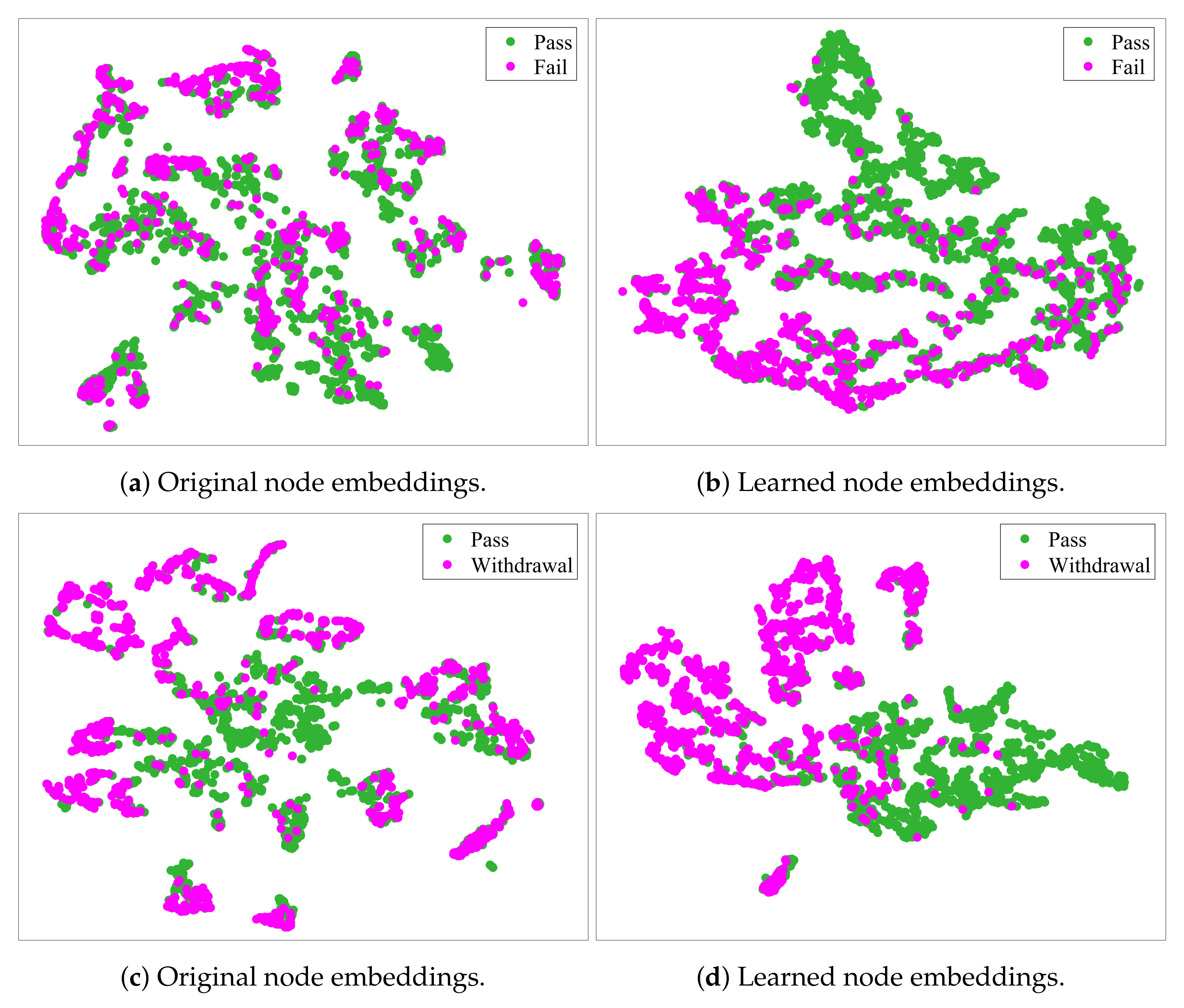
The prediction metrics results are presented in

Table 4. Performance comparison between the baseline models and MTGNN for predicting at-risk students. Bold font indicates the best performance.

Metrics	Categories	SVM	LR	SLFNN	GCN-Cosine	GCN-Pearson	MTGNN
Accuracy	Pass/Fail	80.66	80.25	76.95	80.86	81.48	84.98
	Pass/Withdrawal	87.93	87.78	81.42	88.08	87.31	91.95
F1-score	Pass/Fail	68.67	68.00	45.80	67.82	68.75	73.65
	Pass/Withdrawal	88.39	88.08	78.80	88.06	87.46	92.59
Recall	Pass/Fail	66.88	66.23	29.87	62.42	63.03	68.46
	Pass/Withdrawal	93.69	92.11	70.35	88.47	89.10	97.60

. We can see that our MTGNN model significantly outperforms the baseline models in the two prediction tasks. In particular, the MTGNN model works better than the single-topology GCN (GCN-Cosine and GCN-Pearson) in all three evaluation metrics, which also proves the superiority of multi-topology in practice. Our MTGNN model considers the embedding information of two graphs when modeling and the fused embedding information is captured by the model, so its predictive performance improves. We also visualized node embeddings as shown in Figure 2. Compared with the node embeddings not learned by MTGNN, the learned node embeddings have a more compact structure and clearer boundaries between different categories, showing that our model can cluster nodes of the same category well.

Task 2: Early prediction for at-risk students. The second experiment investigates whether MTGNN has a better performance than the baseline models in early prediction tasks. The early prediction of students’ performance is an important way to improve their learning efficiency. If we can identify students who are at risk of failing or dropping out early in a course, teachers can provide them with timely help and advice, giving them enough time to improve their abilities and understanding. In addition, outstanding students can improve their grades significantly with better-customized study plans. This is why our second experiment is designed to predict student performance early in the course.

We made predictions for at-risk students at weeks 5, 10, 15 and 20, respectively, which also helped us evaluate our models more comprehensively. Similar to Experiment 1, we identify students who are at risk of failure early in the course by dividing students into either Pass or Fail, and to identify students who are at risk of dropping out early in the course, we divide students Pass or Withdrawal. As shown in

Table 5. Performance comparison between the baselines and MTGNN for early prediction task. Bold font indicates the best records.

Moment	Categories	SVM	LR	SLFNN	GCN-Cosine	GCN-Pearson	MTGNN
Week5	Pass/Fail	72.40	72.82	74.31	72.82	73.46	76.22
	Pass/Withdrawal	67.57	68.84	67.25	68.53	68.37	72.20
Week10	Pass/Fail	74.79	77.54	72.25	72.67	73.09	78.39
	Pass/Withdrawal	70.49	72.57	75.28	74.64	75.44	76.40
Week15	Pass/Fail	74.58	76.27	73.73	75.64	76.69	79.24
	Pass/Withdrawal	74.00	74.80	72.41	73.68	72.57	77.67
Week20	Pass/Fail	79.02	78.60	74.15	78.81	77.97	80.72
	Pass/Withdrawal	77.35	78.31	74.32	79.11	79.27	82.30

, MTGNN still achieves better prediction performance compared with the baseline models. From Figure 3, we can clearly see that the prediction accuracy increases with the prediction time, which also proves that as the course progresses, more academic information can be used to improve the prediction accuracy, and by the twentieth week of the course, our model MTGNN achieves 81.14% accuracy on the task of predicting students at risk of failing, and it achieves 82.30% accuracy on the task of predicting students at risk of dropping out, indicating the possibility of the early prediction of students at risk of failing and dropping out. This also shows the effectiveness of the MTGNN model for early intervention, which is of great significance for solving students’ problems in a timely manner and motivating them to continue learning.

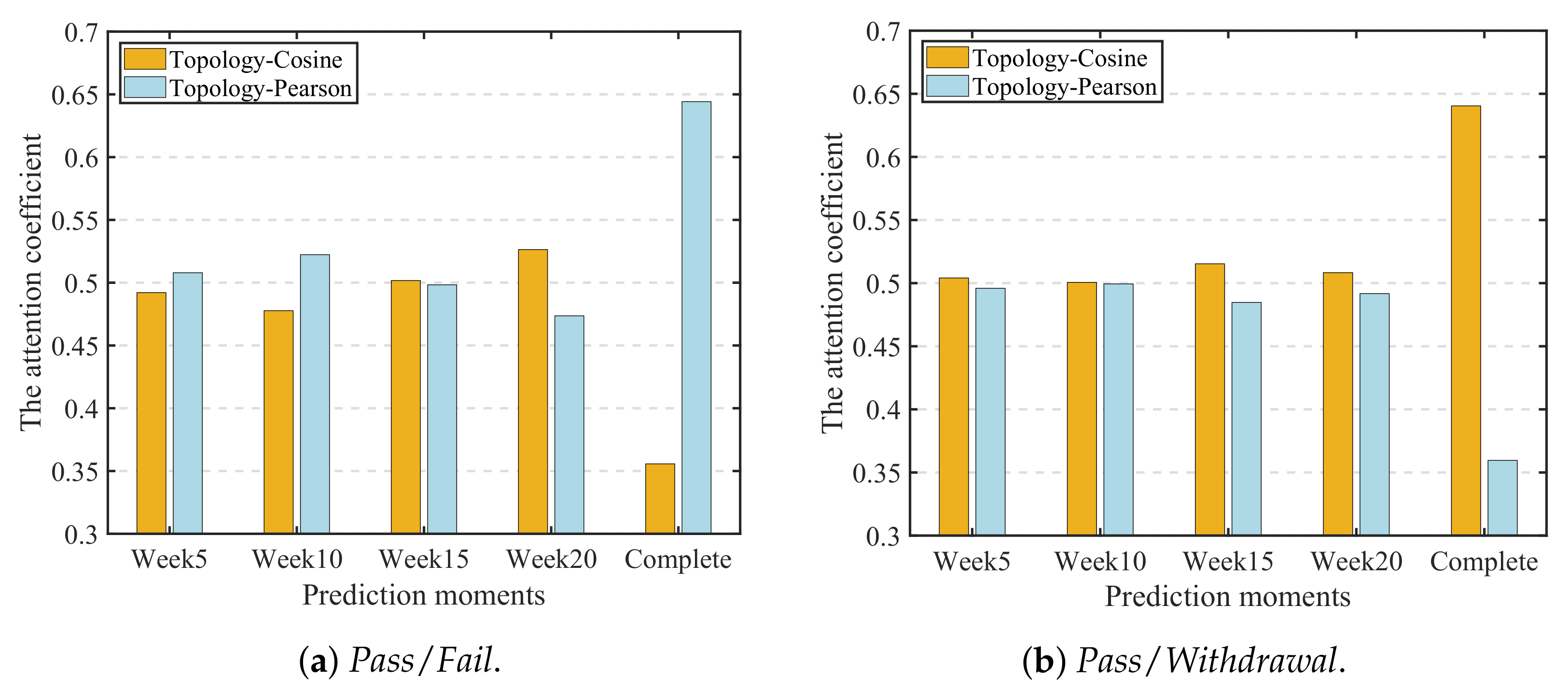
Effects of different student relationship graphs on the prediction performance of MTGNN. The third experiment explores the effects of graphs generated using different similarity learning methods on the predictive performance of MTGNN. In the previous two experiments, we used Cosine and Pearson coefficient to construct two graphs, which we call Topology-Cosine and Topology-Pearson. To answer the third research question, we output the number of edges of each graph and its adaptive importance weight learned by the attention mechanism based on experiments 1 and 2.

From Figure 4, we can see the attention coefficients of the embedding of each graph at different prediction moments in different prediction tasks, and the attention coefficient represents the importance weights of each embedding in the prediction task of the model. Taking the complete time as an example, in the task of predicting failing students, the attention coefficient of Topology-Pearson is larger than Topology-Cosine, which shows that Topology-Pearson provides more useful information in this prediction task. However, in the task of predicting students who are at risk of dropping out, Topology-Cosine has a larger attention coefficient, indicating that it plays a greater role in this task. The importance of graphs constructed using different similarity learning methods varies in different prediction tasks, which shows that our prediction model can adaptively adjust the importance weight of each input graph and realize the effective integration of embeddings to achieve the best prediction effect.

Different similarity learning methods have their own calculation methods and measurement characteristics. Pearson coefficient is used to measure the linear correlation between two variables, and Cosine measures the similarity between two vectors by measuring the cosine of the angle between them. Therefore, the graphs constructed by each are different.

Table 6. A summary of edge numbers for both Cosine and Pearson-based similarity learning.

Moment	Categories	Topology-Cosine	Topology-Pearson
Week5	Pass/Fail	45,142	41,841
	Pass/Withdrawal	104,028	99,389
Week10	Pass/Fail	36,770	33,972
	Pass/Withdrawal	168,404	160,931
Week15	Pass/Fail	37,486	33,698
	Pass/Withdrawal	71,774	66,989
Week20	Pass/Fail	38,402	33,818
	Pass/Withdrawal	77,188	71,147
Complete	Pass/Fail	72,456	65,562
	Pass/Withdrawal	260,434	245,560

shows the number of edges of the student relationship graph under different prediction tasks. It can be seen that there is no correlation between the number of edges and the attention coefficient. This shows that the importance of the student relationship graphs in the prediction task is independent of their size.

The well-known Spearman’s nonparametric correlation analysis [46] was performed to quantify the correlation strength between student performance and the concerned features detailed in Table 3. As shown in

Table 7. Correlation using Spearman’s Rho coefficient for two cases of problem-formulation: Pass (P)/Fail (F), Pass (P)/Withdrawal (W).

Features	P/F	P/W	Features	P/F	P/W
forumng	$0.398$ **	$0.523$ **	url	$0.395$ **	$0.579$ **
homepage	$0.523$ **	$0.729$ **	gender	$-0.086$ **	$-0.031$
oucollaborate	$0.214$ **	$0.313$ **	region	$-0.055$ **	$-0.026$
oucontent	$0.267$ **	$0.391$ **	highest_education	$-0.052$ *	$-0.091$ **
page	$0.476$ **	$0.717$ **	age_band	$0.066$ **	$0.041$ *
quiz	$0.501$ **	$0.740$ **	num_of_prev_attempts	$-0.071$ **	$-0.053$ **
resource	$0.461$ **	$0.682$ **	studied_credits	$0.042$ *	$-0.124$ **
subpage	$0.509$ **	$0.748$ **	disability	0.017	$-0.045$ *

** p < 0.01, * p < 0.05.

, for both the two cases of problem-formulation (Pass/Fail and Pass/Withdrawal), students’ final performance displayed a statistically significant association with some features reflecting the students’ learning behavior, engagement and duration, such as ‘forumng’, ‘homepage’, ‘oucollaborate’, ‘oucontent’, ‘page’, ‘quiz’, ‘resource’, ‘subpage’, ‘url’. This finding is consistent with the ones presented in the related works [9,13,15].

Technically, among the compared baselines, the three conventional methods, i.e., SVM, LR, and SLFNN, do not use the graph data since they are not graph-based approaches and cannot leverage the graph information during the training process. Another baseline, the GCN model (GCN-Cosine, GCN-Pearson) only used a single view of graph topology, where the way to construct the graph topology is the same as that of our proposed MTGNN model. By comparing MTGNN with all these baselines, we can verify straightforwardly the effectiveness of our proposed method in two aspects: (i) GNN-based methods have a good potential to perform better than the conventional approaches that do not consider the graph information (e.g., a connection between students); (ii) GNNs with Multi-Topologies (e.g., our proposed MTGNN) outperform GNNs with single graph topology (e.g., the vanilla GCN model), as demonstrated in Table 4 and Table 5.

Overall, compared with other predictive models, our MTGNN model pays more attention to mining the potential relationship between students and achieves the best accuracy in different prediction tasks, which shows that our model has a satisfactory effect in identifying at-risk students. Effective identification of high-risk students can not only achieve more accurate personalized learning services, but it can also reduce the cost of education investment.

Further remark: To the best of our knowledge, our proposed Study-GNN is the first work presenting a pipeline for dealing with student performance prediction tasks. Specifically, the main focus and technical novelty differ clearly from some existing works. For example, ref. [47] proposed a framework (named student-performulator) to design a student performance prediction model based on deep neural networks (DNNs). Although their framework can be viewed as a pipeline for problem-solving, the authors did not consider graph-based methods when designing the DNN-based models. Ref. [48] developed transfer learning-based DNNs for predicting student performance. Ref. [49] studied the feature selection issue for pre-course student performance prediction. Both of these methods did not touch on the topic of graph neural networks (GNNs), which to some extent limits the promotion of advanced technologies (GNN is the representative one) and applications in ‘AI + Education’. Ref. [50] systematically reviewed the related works for student performance prediction using machine learning techniques. However, GNNs and their variants, as newly-developed methods/tools, were not mentioned in the survey. Based on these aspects, our work moves a step forward by filling the gap between GNNs (as advanced tools in AI) and the (as a classic task that has received wide attention in education).

5. Conclusions

Student performance prediction is an important issue in the current educational research field. However, most current prediction methods treat students individually and do not take into account the correlation of the performance among students with similar characteristics. This paper proposes a novel pipeline for student performance prediction based on a newly-developed multi-topology graph neural network (MTGNN). Specifically, we formalize student performance prediction as a node classification problem in a student graph consisting of student nodes. To better capture the potential relationships among students, we use different similarity learning methods to construct multiple graphs of the student data. Then, we design an MTGNN with a shared parameter strategy based on the GNN model and introduce an attention mechanism to fuse the embeddings in the information transfer stage. We conduct a detailed evaluation of the model’s predictive performance on the OULA dataset by comparing it with four baseline models (SVM, LR, SLFNN, and GCN). The experiment results show that our method has high accuracy and generality.

Future work can focus on the following aspects: (i) the graph construction procedure can be enhanced by considering structure learning along with the model training process and certain constraints for optimizing the adjacency matrices are expected, which has a good potential to improve significantly the capability of multi-topology (or multi-view) GNNs; (ii) comprehensive theoretical analysis on how and why GNNS with multi-topologies outperform the ones with only single topology is meaningful; (iii) it is interesting to further explore whether the proposed method is applicable to other analytical tasks in educational research. Furthermore, it is meaningful to explore how to build a pre-trained model using our pipeline, by which the user can perform fine-tuning (e.g., transferring the ’knowledge’ of the pre-trained model to the new scenario/task) for problem-solving.

References

- Papamitsiou, Z.; Economides, A.A. Learning analytics and educational data mining in practice: A systematic literature review of empirical evidence. J. Educ. Technol. Soc. 2014, 17, 49–64. [Google Scholar]
- Pelletier, K.; Brown, M.; Brooks, D.C.; McCormack, M.; Reeves, J.; Arbino, N.; Bozkurt, A.; Crawford, S.; Czerniewicz, L.; Gibson, R.; et al. 2021 EDUCAUSE Horizon Report Teaching and Learning Edition; EDU: Boulder, CO, USA, 2021. [Google Scholar]
- Tomasevic, N.; Gvozdenovic, N.; Vranes, S. An overview and comparison of supervised data mining techniques for student exam performance prediction. Comput. Educ. 2020, 143, 103676. [Google Scholar] [CrossRef]
- Romero, C.; Ventura, S. Educational data mining: A survey from 1995 to 2005. Expert Syst. Appl. 2007, 33, 135–146. [Google Scholar] [CrossRef]
- Marbouti, F.; Diefes-Dux, H.A.; Strobel, J. Building course-specific regression-based models to identify at-risk students. In Proceedings of the ASEE Annual Conference and Exposition, Seattle, WA, USA, 14–17 June 2015; pp. 26–304. [Google Scholar]
- Arsad, P.M.; Buniyamin, N. A neural network students’ performance prediction model (NNSPPM). In Proceedings of the IEEE International Conference on Smart Instrumentation, Measurement and Applications, Kuala Lumpur, Malaysia, 25–27 November 2013; pp. 1–5. [Google Scholar]
- Xu, X.; Wang, J.; Peng, H.; Wu, R. Prediction of academic performance associated with internet usage behaviors using machine learning algorithms. Comput. Hum. Behav. 2019, 98, 166–173. [Google Scholar] [CrossRef]
- Yang, Z.; Yang, J.; Rice, K.; Hung, J.L.; Du, X. Using convolutional neural network to recognize learning images for early warning of at-risk students. IEEE Trans. Learn. Technol. 2020, 13, 617–630. [Google Scholar] [CrossRef]
- Riestra-González, M.; del Puerto Paule-Ruíz, M.; Ortin, F. Massive LMS log data analysis for the early prediction of course-agnostic student performance. Comput. Educ. 2021, 163, 104108. [Google Scholar] [CrossRef]
- Hu, Q.; Rangwala, H. Academic performance estimation with attention-based graph convolutional networks. In Proceedings of the 12th International Conference on Educational Data Mining, Montreal, QC, Canada, 2–5 July 2019; pp. 69–78. [Google Scholar]
- Karimi, H.; Derr, T.; Huang, J.; Tang, J. Online academic course performance prediction using relational graph convolutional neural network. In Proceedings of the 13th International Conference on Educational Data Mining, Virtual, 10–13 July 2020; pp. 444–450. [Google Scholar]
- Li, H.; Wei, H.; Wang, Y.; Song, Y.; Qu, H. Peer-inspired student performance prediction in interactive online question pools with graph neural network. In Proceedings of the 29th ACM International Conference on Information and Knowledge Management, Virtual Event, Ireland, 19–23 October 2020; pp. 2589–2596. [Google Scholar]
- Kuzilek, J.; Hlosta, M.; Zdrahal, Z. Open university learning analytics dataset. Sci. Data 2017, 4, 1–8. [Google Scholar] [CrossRef] [Green Version]
- Martinho, V.R.; Nunes, C.; Minussi, C.R. Prediction of school dropout risk group using neural network. In Proceedings of the Federated Conference on Computer Science and Information Systems, Krakow, Poland, 8–11 September 2013; pp. 111–114. [Google Scholar]
- Waheed, H.; Hassan, S.U.; Aljohani, N.R.; Hardman, J.; Alelyani, S.; Nawaz, R. Predicting academic performance of students from VLE big data using deep learning models. Comput. Hum. Behav. 2020, 104, 106189. [Google Scholar] [CrossRef] [Green Version]
- Costa, E.B.; Fonseca, B.; Santana, M.A.; de Araújo, F.F.; Rego, J. Evaluating the effectiveness of educational data mining techniques for early prediction of students’ academic failure in introductory programming courses. Comput. Hum. Behav. 2017, 73, 247–256. [Google Scholar] [CrossRef]
- Ren, Z.; Rangwala, H.; Johri, A. Predicting performance on MOOC assessments using multi-regression models. In Proceedings of the 9th International Conference on Educational Data Mining, Raleigh, NC, USA, 29 June–2 July 2016; pp. 484–489. [Google Scholar]
- Yang, F.; Li, F.W. Study on student performance estimation, student progress analysis, and student potential prediction based on data mining. Comput. Educ. 2018, 123, 97–108. [Google Scholar] [CrossRef] [Green Version]
- Chui, K.T.; Fung, D.C.L.; Lytras, M.D.; Lam, T.M. Predicting at-risk university students in a virtual learning environment via a machine learning algorithm. Comput. Hum. Behav. 2020, 107, 105584. [Google Scholar] [CrossRef]
- Scarselli, F.; Gori, M.; Tsoi, A.C.; Hagenbuchner, M.; Monfardini, G. The graph neural network model. IEEE Trans. Neural Netw. 2009, 20, 61–80. [Google Scholar] [CrossRef] [Green Version]
- Bacciu, D.; Errica, F.; Micheli, A.; Podda, M. A gentle introduction to deep learning for graphs. Neural Netw. 2020, 129, 203–221. [Google Scholar] [CrossRef]
- Zhou, J.; Cui, G.; Hu, S.; Zhang, Z.; Yang, C.; Liu, Z.; Wang, L.; Li, C.; Sun, M. Graph neural networks: A review of methods and applications. AI Open 2020, 1, 57–81. [Google Scholar] [CrossRef]
- Wu, Z.; Pan, S.; Chen, F.; Long, G.; Zhang, C.; Yu, P.S. A comprehensive survey on graph neural networks. IEEE Trans. Neural Netw. Learn. Syst. 2021, 32, 4–24. [Google Scholar] [CrossRef] [Green Version]
- Zhang, Z.; Cui, P.; Zhu, W. Deep learning on graphs: A survey. IEEE Trans. Knowl. Data Eng. 2022, 34, 249–270. [Google Scholar] [CrossRef] [Green Version]
- Nakagawa, H.; Iwasawa, Y.; Matsuo, Y. Graph-based knowledge tracing: Modeling student proficiency using graph neural network. In Proceedings of the IEEE/WIC/ACM International Conference on Web Intelligence, Thessaloniki, Greece, 14–17 October 2019; pp. 156–163. [Google Scholar]
- Song, X.; Li, J.; Tang, Y.; Zhao, T.; Chen, Y.; Guan, Z. JKT: A joint graph convolutional network based deep knowledge tracing. Inf. Sci. 2021, 580, 510–523. [Google Scholar] [CrossRef]
- Yang, Y.; Shen, J.; Qu, Y.; Liu, Y.; Wang, K.; Zhu, Y.; Zhang, W.; Yu, Y. GIKT: A graph-based interaction model for knowledge tracing. In Proceedings of the Joint European Conference on Machine Learning and Knowledge Discovery in Databases, Ghent, Belgium, 14–18 September 2020; pp. 299–315. [Google Scholar]
- Abdelrahman, G.M.; Wang, Q. Deep graph memory networks for forgetting-robust knowledge tracing. arXiv 2021, arXiv:2108.08105. [Google Scholar]
- Gan, W.; Sun, Y.; Sun, Y. Knowledge structure enhanced graph representation learning model for attentive knowledge tracing. Int. J. Intell. Syst. 2022, 37, 2012–2045. [Google Scholar] [CrossRef]
- Song, X.; Li, J.; Lei, Q.; Zhao, W.; Chen, Y.; Mian, A. Bi-CLKT: Bi-graph contrastive learning based knowledge tracing. Knowl.-Based Syst. 2022, 241, 108274. [Google Scholar] [CrossRef]
- Gao, W.; Liu, Q.; Huang, Z.; Yin, Y.; Bi, H.; Wang, M.C.; Ma, J.; Wang, S.; Su, Y. RCD: Relation map driven cognitive diagnosis for intelligent education systems. In Proceedings of the 44th ACM SIGIR Conference on Research and Development in Information Retrieval, Virtual Event, Canada, 11–15 July 2021; pp. 501–510. [Google Scholar]
- Mao, Y.; Xu, B.; Yu, J.; Fang, Y.; Yuan, J.; Li, J.; Hou, L. Learning Behavior-Aware Cognitive Diagnosis for Online Education Systems. In Proceedings of the International Conference of Pioneering Computer Scientists, Engineers and Educators, Taiyuan, China, 17–20 September 2021; pp. 385–398. [Google Scholar]
- Zhang, J.; Mo, Y.; Chen, C.; He, X. GKT-CD: Make cognitive diagnosis model enhanced by graph-based knowledge tracing. In Proceedings of the International Joint Conference on Neural Networks, Shenzhen, China, 18–22 July 2021; pp. 1–8. [Google Scholar]
- Tan, H.; Wang, C.; Duan, Q.; Lu, Y.; Zhang, H.; Li, R. Automatic short answer grading by encoding student responses via a graph convolutional network. Interact. Learn. Environ. 2020, 1–15. [Google Scholar] [CrossRef]
- Kipf, T.N.; Welling, M. Semi-supervised classification with graph convolutional networks. In Proceedings of the International Conference on Learning Representations, Toulon, France, 24–26 April 2017. [Google Scholar]
- Defferrard, M.; Bresson, X.; Vandergheynst, P. Convolutional neural networks on graphs with fast localized spectral filtering. In Proceedings of the Annual Conference on Neural Information Processing Systems 2016, Barcelona, Spain, 5–10 December 2016. [Google Scholar]
- Bruna, J.; Zaremba, W.; Szlam, A.; LeCun, Y. Spectral networks and locally connected networks on graphs. In Proceedings of the International Conference on Learning Representations, Banff, AB, Canada, 14–16 April 2014. [Google Scholar]
- Mallat, S. A Wavelet Tour of Signal Processing; Elsevier: Amsterdam, The Netherlands, 1999. [Google Scholar]
- Shuman, D.I.; Narang, S.K.; Frossard, P.; Ortega, A.; Vandergheynst, P. The emerging field of signal processing on graphs: Extending high-dimensional data analysis to networks and other irregular domains. IEEE Signal Process. Mag. 2013, 30, 83–98. [Google Scholar] [CrossRef] [Green Version]
- Chung, F.R.; Graham, F.C. Spectral Graph Theory; American Mathematical Society: Providence, RI, USA, 1997. [Google Scholar]
- Henaff, M.; Bruna, J.; LeCun, Y. Deep convolutional networks on graph-structured data. arXiv 2015, arXiv:1506.05163. [Google Scholar]
- Cha, S.H. Comprehensive survey on distance/similarity measures between probability density functions. Int. J. Math. Model. Methods Appl. Sci. 2007, 1, 300–307. [Google Scholar]
- Veličković, P.; Cucurull, G.; Casanova, A.; Romero, A.; Lio, P.; Bengio, Y. Graph attention networks. In Proceedings of the International Conference on Learning Representations, Vancouver, BC, Canada, 30 April–3 May 2018. [Google Scholar]
- McPherson, M.; Smith-Lovin, L.; Cook, J.M. Birds of a feather: Homophily in social networks. Annu. Rev. Sociol. 2001, 27, 415–444. [Google Scholar] [CrossRef] [Green Version]
- Mohri, M.; Rostamizadeh, A.; Talwalkar, A. Foundations of Mchine Learning; MIT Press: Cambridge, UK, 2018. [Google Scholar]
- Fielden, J.D.G.; Gibbons, J.D. Nonparametric Measures of Association; SAGE: New York, NY, USA, 1993; Number 91. [Google Scholar]
- Yousafzai, B.K.; Khan, S.A.; Rahman, T.; Khan, I.; Ullah, I.; Ur Rehman, A.; Baz, M.; Hamam, H.; Cheikhrouhou, O. Student-performulator: Student academic performance using hybrid deep neural network. Sustainability 2021, 13, 9775. [Google Scholar] [CrossRef]
- Tsiakmaki, M.; Kostopoulos, G.; Kotsiantis, S.; Ragos, O. Transfer learning from deep neural networks for predicting student performance. Appl. Sci. 2020, 10, 2145. [Google Scholar] [CrossRef] [Green Version]
- Yang, J.; Hu, S.; Wang, Q.; Fong, S. Discriminable Multi-Label Attribute Selection for Pre-Course Student Performance Prediction. Entropy 2021, 23, 1252. [Google Scholar] [CrossRef] [PubMed]
- Albreiki, B.; Zaki, N.; Alashwal, H. A systematic literature review of student’s performance prediction using machine learning techniques. Educ. Sci. 2021, 11, 552. [Google Scholar] [CrossRef]
Figure 1.
The whole framework of MTGNN for student performance prediction. The pipeline includes four main procedures: data collection, data pre-processing, graph construction based on similarity learning, and the proposed Multi-Topology Graph Neural Networks (MTGNN) for semi-supervised node classification.
Figure 2.
Visualization of node embeddings: (a) original embeddings for categories Pass/Fail; (b) learned embeddings by MTGNN for categories Pass/Fail; (c) original embeddings for categories Pass/Withdrawal; (d) learned embeddings by MTGNN for categories Pass/Withdrawal.
Figure 3.
MTGNN’s test accuracies for early prediction of at-risk students (e.g., Fail, Withdrawal).
Figure 4.
Attention coefficients configured for topologies used in MTGNN.