
Real-Time Vehicle Detection Based on Improved YOLO v5
by
 , ,
, ,
Yu Zhang
1,
Zhongyin Guo
1,
Jianqing Wu
2,3,
Yuan Tian
2,3,*,
Haotian Tang
2 and
Xinming Guo
2,3,* 1
Key Laboratory of Road and Traffic Engineering of the Ministry of Education, Tongji University, Shanghai 201804, China
2
School of Qilu Transportation, Shandong University, Jinan 250061, China
3
Suzhou Research Institute, Shandong University, Suzhou 215000, China
*
Authors to whom correspondence should be addressed.
Sustainability 2022, 14(19), 12274; https://doi.org/10.3390/su141912274
Submission received: 8 August 2022
/
Revised: 20 September 2022
/
Accepted: 26 September 2022
/
Published: 27 September 2022
Abstract
:To reduce the false detection rate of vehicle targets caused by occlusion, an improved method of vehicle detection in different traffic scenarios based on an improved YOLO v5 network is proposed. The proposed method uses the Flip-Mosaic algorithm to enhance the network’s perception of small targets. A multi-type vehicle target dataset collected in different scenarios was set up. The detection model was trained based on the dataset. The experimental results showed that the Flip-Mosaic data enhancement algorithm can improve the accuracy of vehicle detection and reduce the false detection rate.
1. Introduction
By the end of 2020, the total mileage of freeways in China reached 161,000 km, ranking first in the world [1]. With the development of the new generation of technology, the information-based and data-based smart expressway has been piloted. The smart expressway can improve traffic safety and efficiency. Additionally, the smart freeway allows vehicle–road collaboration by building an efficient communication system between the cloud platform, roadside infrastructure, road users, and big data centers.
Although the construction of the Chinese expressway network is becoming more intelligent, and comprehensive traffic management technology is improving rapidly, there are still some challenges that need to be solved. On 1 January 2020, China completed the cancellation of the whole network of the expressway provincial border toll station project. The expressway realized the “one network” operation mode of “one pass, one deduction, one notification” [2], and the whole network system adopted segmented billing. The charging mode was changed from weight charging to per-vehicle charging, and the billing mileage was determined by the ETC system and the toll booths according to the driving path. Under the new toll collection system, the expressway toll system faces the problem of evading tolls and difficult recovery. Moreover, compared with urban arterial roads, the expressway has the characteristics of fast speed, large traffic capacity, and a high volume of commercial trucks with dangerous goods. Although the accident rate is relatively low, the harm caused by traffic accidents on the expressway is more serious [3], and the subsequent effects, such as congestion caused by accidents, last longer.
Vehicle target detection on the expressway is important for intelligent traffic management and safety monitoring. It is the basis for realizing intelligent and diversified traffic management. Relying on manual supervision is inefficient, and it can only be analyzed after the event has occurred. Some traditional intelligent monitoring systems have a high false-positive rate and a slow speed. The early warning information usually has a high false rate. Since 2006, the rise of deep learning has enabled computer vision technology to develop from manual design features to higher precision and intelligence [4], which also provides technical support for the real-time, full, and efficient use of surveillance videos. Vehicle category detection by monitoring video streams can strengthen the operation and maintenance supervision of expressways and improve vehicle driving efficiency and safety. It is of great significance for ensuring the safety of people’s lives and property and the development of the economy.
2. Related Work
Vehicle detection is used to detect the vehicle target from the inspected area and accurately classify the vehicle type to accurately locate the vehicle position [5]. Object detection has always been a hotspot in the field of computer vision, and vehicle detection has always been the most basic and arduous task in the field of object detection due to the vehicle appearance attributes and different states in the detection process [6].
Traditional vehicle detection algorithms usually extract features by manual extraction. The moving vehicles are extracted from video sequences and then the extracted features are classified by the classifier to achieve the purpose of vehicle identification. Vehicle detection methods mainly include the background update method [6], the frame difference method [7], and the optical flow method [8]. The background update method uses the idea of a weighted average to update the background, and the effect of the background update often affects the completeness of target extraction and the accuracy of target detection [9]. The frame difference method aims to achieve the purpose of target extraction by calculating the difference between adjacent frames. This method is often greatly influenced by the speed of the vehicle and the time interval between successive frames [10]. The optical flow method is a density estimation approach at the pixel level [11]. The first step in the inspection process is to use sliding windows of different sizes to generate a large number of candidate boxes in the tested area. Then the features are selected in this candidate box. Finally, the classification controller is used to classify and accurately locate the specific location of each target in this candidate box. However, the huge amount of computation is very unfavorable to the real-time detection of targets. Commonly, the detection features used for vehicle detection are SIFT, HOG, Harr, etc. [12,13,14,15]. Classification controller devices include SVM and Adaboost, etc. [16,17]. The vehicle detection modes include Harr + Adaboost, Hog + SVM, and DPM [18]. The traditional method of selecting features relies on prior knowledge. In the actual application of the scene, there are many objective interference factors including lighting, deformation, etc. Therefore, it is difficult for traditional vehicle detection algorithms to be applied to real scenes, and it is difficult to achieve the accuracy and robustness necessary for practical applications [19,20,21].
The vehicle detection methods that are widely used can be divided into two categories. One is the R-CNN series of operation methods based on the two stages of the candidate region. The first step of the two-stage method is generating a candidate box in a certain way. Then, the contents of the candidate box are discriminated against and classified, and the position of the candidate box is corrected. It is called the two-stage method because it consists of two parts, namely, generating candidate regions and detecting them. CNN was originally applied to the field of object detection as the two-stage approach. R-CNN [22] proposed by RBG (Ross Girshick) et al. was the earliest method to use CNN to achieve target detection. The R represented Region, and R-CNN was “Regions with CNN features”. It was a method in which the features were extracted using CNNs in candidate regions screened in a certain way and then the detection targets were classified. Because CNN performed well in whole image classification tasks, it was used in the field of object detection, and its powerful feature extraction capability was applied to more difficult tasks than integer classification. SPP-net [23] was published by Kaiming He et al. in 2014. The biggest improvement of the SPP-net was that the method of spatial pyramid pooling was proposed. The improved method proposed a solution for the problem in which each candidate region in the R-CNN underwent a CNN feature calculation, and a significant increase in detection speed was achieved. It also solved the problem of target shape distortion as there is no need to scale the detection image to match the input size of the CNN. The images under test in the SPP-NET only needed to undergo one CNN calculation. Feature extraction was performed on the full image of the inspection image. Moreover, the selections of candidate areas were not directly performed in the original map, and they were performed on the feature layer surface extracted by CNN. Fast R-CNN [24] was an improved version that RBG referenced to the previously proposed R-CNN based on SPP-NET. The feature map of the entire ROI extracted features directly, resulting in an efficiency improvement. Faster R-CNN [25] was further optimized for detecting slow speeds in Fast R-CNN. The main improvement was the use of RPN networks instead of the traditional Selective Search approach to generating candidate boxes. In addition, the concept of the anchor was introduced, which had been used in later models.
Unlike the two-stage method, the one-stage method does not require candidate boxes to be generated in advance. Instead, candidate boxes are predicted and classified directly at various locations in the image. The most representative examples of single-stage approaches are SSD [26] and YOLO [27]. In 2016, Liu et al. proposed SSD (Single-Shot MultiBox Detector). The algorithm detected objects of different scales at different layers of the network, and other algorithms run the detection section only at the top level of the network. Since then, there have been many improved versions of the SSD algorithm. SSD was the more comprehensive one-phase object detection method after YOLO. SSD was improved in the following two points: j The detection targets were pre-framed and the scales and proportions of the pre-check box were given. In fact, the effect was equivalent to the anchor box proposed in the previous Faster R-CNN. k Multi-scale classification is when the feature maps of CNN output were used to make classification predictions on different scales. YOLO was characterized by its speed, but it was not effective when detecting small objects, and the positioning was not accurate. In 2015, Joseph [6] proposed the first single-stage detector. YOLO (You Only Look Once) reached the speed of 45fps and its accuracy surpassed RCNN. Its fast version reached 155fps. It opened the era of single-stage detection algorithms and provided technical support for the deployment and application of target detection in the industrial industry. YOLO proposed a completely new design idea that applied CNN to entire images. It predicted target classifications and bounding boxes with direct regression of output features. The original author made a series of improvements on the basis of YOLO and successively proposed the YOLO9000 [28] and YOLO v3 [29], adding FPN and other structures to improve the loss function. In 2020, AlexAB released YOLO v4 [30]. A variety of data enhancement methods in the field of computer vision were integrated, and various new backbone network combinations were tried. It applied the Mish activation function, Drop block prevention overfit policies, the combination of FPN and the PAN network, and improvements in the bounding box loss function CIOU_Loss. The average accuracy of the COCO dataset was 10 percentage points higher than that of YOLO v3. In the same year, Jocher Glenn released version 5 of YOLO [31]. Although the naming was not officially recognized, its actual performance was further improved. From the rapid development of the YOLO series algorithm in recent years, it can be seen that both academia and industry have great interest and expectations for this algorithm. Many scholars’ research progress in object detection focuses on the improved optimization algorithm based on the YOLO algorithm. They put forward some difficult problems and research trends in the field of object detection. In addition, the problem of small object detection in the field of object detection was analyzed systematically. A variety of algorithms are introduced across the five aspects of multi-scale, feature resolution improvement, contextual semantic information, data enhancement, and network optimization. The characteristics of algorithms and networks are compared.
For highway application scenarios, this paper further improved the detection accuracy by using the Flip-Mosaic algorithm to monitor video streams based on the improved YOLO v5 algorithm. Furthermore, a multi-type vehicle target dataset for multiple kinds of weather and scenarios was developed. According to the dataset, the detection model of real-time detection of vehicle category information was obtained. The study has important practical significance for the supervision of expressways’ operation status and the improvement of the transportation department’s management service level.
3. Data Collection and Data Processing
There are four types of problems in vehicle target detection.
- (1)
- Due to the different installation scenarios of traffic monitoring, there are differences in the viewing angle and height of monitoring, which will produce scene changes. For example, the monitoring perspective and scene characteristics in the tunnel are different from the highway. This discrepancy leads to a significant reduction in the detection accuracy and also leads to a large number of vehicle targets missing inspection.
- (2)
- The same scene in different weather conditions also varies greatly. Affected by the brightness of the scene picture under bad weather conditions and the noise of the camera acquisition equipment, the body contour feature extraction of the target vehicle is susceptible to interference. If the dataset does not contain such scene data, the detection effect is not ideal.
- (3)
- The vehicle target has noticeable deformation in different positions in the picture. The same vehicle target undergoes significant size deformation at the distal and proximal positions of the picture. It affects the detection accuracy of small targets.
- (4)
- Vehicle occlusion is common to vehicle targets on actual roads, which can lead to the detection of multiple targets as a single target, and there are missed and false detections.
3.1. Data Collection
Open-source datasets are often constructed by the authors according to the research needs of the time, and the characteristics of the data may not strictly meet the requirements of the current research. As research in a specific domain requires datasets under specific scenarios or conditions, this paper establishes some datasets to verify its own research. According to the characteristics of expressway monitoring application angle [32] and resolution, the multi-angle monitoring video of a certain point of the Dongying to Jinan section of the Shandong Dongying Expressway and the Yiyuan Tunnel Expressway of the Zibo Expressway in Shandong province was collected. The whole road adopted a two-way four-lane expressway standard, with a design speed of 120 km/h. This is shown in Figure 1.
To ensure the diversity of vehicle samples in the image, the video data were processed to extract one image sample every 40 frames. A total of 1493 pictures with vehicle information were extracted, and the original vehicle detection image library was set with the selection of 1060 pictures of multiple types of vehicles from the BIT Vehicle_Dataset [33]. This dataset contained multiple types of vehicles, such as trucks, family cars, taxis, tankers, and so on. In addition, the video segments used to create the dataset were available at any time of day and night, which ensured the diversity of the dataset. The detection network training dataset was produced through high-definition surveillance videos and multi-type vehicle pictures from different angles, road sections, and lighting conditions. This was used for the training and evaluation of the detection model in Section 3, as shown in Figure 2. Scenario 1 and Scenario 2 were video collection scenarios of a section of Dongying Expressway under different weather conditions. Scenario 3 was a video collection scene of The Yiyuan Tunnel in Zibo. Scenario 4 was a multi-type vehicle image to expand the diversity of the dataset.
3.2. Image Labeling Method for Vehicle Detection
Vehicle inspection is a supervised learning task [34]. Model training requires classification and location information about the vehicle in the image. Regarding the classification of vehicle targets, the practical application of vehicle target detection in highway scenarios was considered. Target vehicles were divided into 8 categories according to the difficulty of distinguishing between vehicle classes in the images captured by the high camera, including Bus, Minibus, Family Sedan, Taxi, Heavy Truck, Truck, SUV, and Special Vehicle. Figure 3 was a schematic diagram of vehicle sample classification in this dataset.
Data labeling is a tedious and repetitive task that must be performed manually, and this article used a semi-automated labeling tool (as shown in Figure 4). Although manual checking and fine-tuning were required, it greatly reduced the complexity of the annotation task.
First, the object detection and labeling tool MakeSense was used to label a part of the image sample in a rectangular box. The tool generated a label file corresponding to the image naming, which was illustrated in Figure 5. The resulting callout file was a txt file. which mainly saved the label category and the upper left right coordinate point information of the rectangular box, as shown in Table 1.
Each line in the YOLO annotation format txt represented the category and position of an object. The first column represented the category of the object. The next four columns represented the position information of the object, which were x, y, w, and h. Each image corresponded to a txt file, and there were multiple categories of objects in one file. X and y were the central coordinates of the target, and w and h were the width and height of the target, respectively. These coordinates were normalized. X and w were normalized using the width of the original diagram, and y and h were normalized using the height of the original diagram. The information about the YOLO annotation categories in this article is shown in Table 2.
This annotation information was then used to train the object detection model. Because the amount of data was small and the model and data were not optimized, it was named the coarse detection model. The coarse detection model was used to detect the remaining unlabeled images through the semi-automatic annotation program [35], which automatically generated a txt text file in the same format as MakeSense. The automatically generated annotation files were manually checked and fine-tuned by the MakeSense tool to complete the detection box annotation of all image sample libraries.
3.3. Image Annotation
The quality of the labeled dataset largely determined how good the model was. In order to train a vehicle detection model that was more in line with the actual highway traffic scenario, the following labeling standard rules were formulated:
- (1)
- Because the object detection task recognizes the part outside the callout box as a negative sample of the background class, the vehicles that appear in the image should be labeled as much as possible, including a small part of the vehicle body that is covered by text information.
- (2)
- In the case of vehicles and the environment, and vehicles obscuring each other, any vehicle of which no more than half is obstructed still needs to be marked. As shown in Figure 6, when that much information is lost, it does not need to be labeled, because such vehicles have basically no target characteristics.
3.4. Dataset Characteristics
To complete the production of the standard dataset, it was necessary to analyze the characteristics of the application scenario of this dataset to optimize and improve the vehicle detection model. Based on statistical labeling information, a plot analysis was performed on the dimensions of the labeled vehicle categories and callout boxes, as shown in Figure 7.
Figure 7 shows the statistics of the number of label categories on the left, and the image on the right shows the density map after the dimensions of the callout box were normalized. There was a serious imbalance in the vehicle categories, as shown in the figure. This was an imbalance in the foreground category in the field of object detection, which had a greater impact on the results of the detection model. The size of the vehicle target in the image was generally small, which was also detrimental to detection.
3.5. Dataset Division
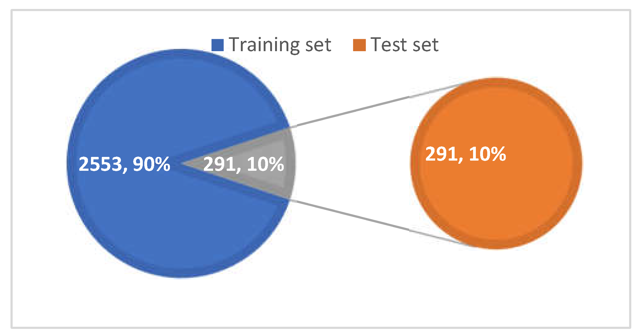
The dataset had a total of 2844 images, as shown in Figure 8. The training sets and validation sets were divided into a 9:1 ratio. In total, 2553 images were used for training validation and 291 images were tested and evaluated by algorithms. In the process of partitioning, one should try to maintain a balance between the number of sample categories in the training verification and test set, and the consistency of the data distribution should be ensured as much as possible.
4. Research on Highway Vehicle Detection Based on Improved YOLO v5 Algorithm
In recent years, with the development of deep learning theory and the upgrade of GPU hardware devices, computer vision technology has also made great progress. Reducing the consumption of manpower through computer vision technology has important practical significance. Object detection is an important basic branch of digital image processing and computer vision, and it is also the core part of intelligent monitoring systems for various application scenarios. After completing the dataset in the previous section, the vehicle detection task still faces the challenge of small object detection. Since the height of the highway surveillance camera is generally 8 m to 12 m, the vehicle target that is located a great distance from the camera in the captured image is relatively small. Because the picture is blurry and there is less information contained, this type of target has always been a practical and common problem in the field of object detection. How to better detect vehicles that are far away from the surveillance camera is of great significance to improving the actual utilization rate of the camera shooting screen.
4.1. YOLO v5 Algorithm
The YOLO object detection algorithm is the first single-stage object detection algorithm proposed by Redmon J. It discards the step of candidate box extraction in the two-stage algorithm and unifies the bounding box and classification into a regression problem. The process of the YOLO algorithm is as follows: First, the image is divided into S × S meshes. Each grid is responsible for predicting the target where the actual box will fall in the center of the grid. A total of S × S × B bounding boxes are generated from these meshes. Each bounding box contains five parameters: Target center point coordinates, target width and height dimensions (x, y, w, h), and confidence of whether the target is contained. S × S grids predict the category probability of the target in that grid. The prediction bounding box confidence and category probability are then multiplied to obtain the category score for each prediction box. These prediction boxes are filtered by non-maximum suppression (NMS) to obtain the final prediction results. The algorithms of the YOLO series have developed rapidly in recent years. In 2020, two versions of YOLO v4 and YOLO v5 appeared successively. The YOLO v5 algorithm achieved a precision accuracy of nearly 50 mAP in the COCO dataset [36] while ensuring the speed of operation. Considering the accuracy and speed requirements of vehicle detection algorithms in highway monitoring scenarios, this chapter selected the s (small) version in YOLO v5 as the benchmark network model. The network model was improved for highway scenarios to further improve the accuracy of the detection algorithm.
YOLO v5 is the most advanced detection network of the YOLO object detection algorithm. Based on the YOLO v3 and YOLO v4 algorithms, the arithmetic set innovation was carried out to improve the detection speed. YOLO v5 borrowed the idea of anchor boxes to improve the speed of the R-CNN algorithm, and manually selected anchor boxes were abandoned. The K-means clustering on the dimensions of the bounding box was run to obtain better a prior value. In 2020, Glenn Jocher released the YOLO v5. The network structure was shown in Figure 9, including input, backbone, neck, and prediction.
- (1)
- The input is a vehicle image input link, which consists of three parts: Data enhancement [37], picture size processing [38], and automatic adaptation anchor frame [39]. The traditional YOLO v5 uses mosaic data enhancement to randomly scale, crop, arrange, and then stitch the input to improve the detection effect of small targets. When training the dataset, the input image size is changed to a uniform size and then the image is fed into the model for inspection. The initial set sizes are set to 460 × 460 × 30. The initial anchor frame for YOLO v5 is (116,90,156,198,373,326).
- (2)
- The backbone network consists of the Focus structure [40] and CSP structure [41]. The Focus structure is responsible for slicing the image before it enters the backbone network. As shown in Figure 10, the original 608 × 608 × 3 image is sliced. The feature map of 304 × 304 × 12 is reached, and then the feature map of the 32 convolutional kernels is formed through the convolutional operation. The Focus operation can downsample the input dimensions without parameters and preserve the original image information as much as possible. The CSP structure is a transition of the input feature using two 1*1 convolutions. It is beneficial for improving the learning ability of CNNs [42], breaking through computing bottlenecks, and reducing memory costs.
- (3)
- The Neck part is a network layer that combines image features and passes them to the prediction layer. The Neck section of YOLO v5 uses the structure of FPN+PAN. The FPN upsamples the high-level feature information and communicates and fuses it in a top-to-bottom manner to obtain a feature map for prediction. PAN is the underlying pyramid, which conveys strong positioning characteristics in a bottom-to-top manner [43].
- (4)
- The prediction layer predicts the image features and generates the bounding box to predict the category. YOLO v5 uses GIOU_Loss as a loss function for Boundingbox. In overlapping object detection, GIOU_NMS is more effective than traditional non-maximum suppression (NMS).
YOLO v5 inherits the meshing ideas of the YOLO algorithm. The network input dimensions are 640 × 640 × 3. That is the three-channel RGB color picture with a length and width of 640 after the original image preprocessing [44]. Passing through the network, the output dimension of the detection layer of the three scales of large, medium, and small is .
is the number of the divided mesh. corresponds to the number of preset prior boxes for each scale. is the number of categories that need to be predicted. The large-scale is an example, where the detection layer output dimension of the network structure of this dimension is 9600.
are the bounding-box-related parameters. is the bounding box confidence. is the confidence of category i. These parameters require the decoding of Formula (1) to obtain the final prediction box [45].
As shown in Figure 11, the blue box is the ground truth box. , , , and are the center point coordinates and width–height dimensions of the label bounding box, respectively. and are the distance between the grid occupied by the center of the label bounding box and the upper left corner of the grid. The red one is the anchor box. and are the width and height of the prior frame.
When training on an object detection task, positive–negative (foreground–background) sample imbalance is a common factor that most affects the performance of the algorithm. YOLO v5 assigns the label box to three anchors at the same time during training, which is equivalent to expanding the positive sample size 3 times. To a certain extent, the problem of positive–negative sample imbalance during the training of the target detection algorithm is alleviated. The loss function is calculated as in Formula (2):
N is the number of detection layers. B is the target number of labels assigned to the prior box. S × S is the number of meshes that are divided into this scale. is the bounding box of regression loss to calculate each target. is the loss of the target object to calculate each mesh. is the classified loss to calculate each target. ,, are the weights of these three losses.
4.2. Improved YOLO v5 Algorithm
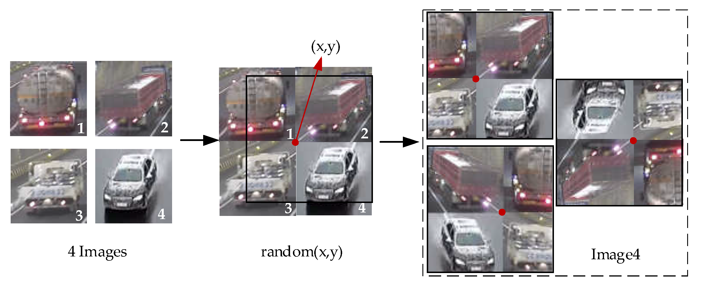
Data quality and quantity are important conditions for the rapid development of deep learning, especially for the learning task of target detection that requires strong supervision. An imbalance in the number of label dataset categories can result in a larger loss of categories, contributing more to the total loss. The loss contribution of a small number of categories is dilute. This reduces the network’s ability to distinguish categories with a small number of labels, resulting in more inaccurate checks and missed inspections in this category. The more effective way to mitigate sample size imbalance is to start at the data input, where each batch of the input network contains a relatively balanced number of categories. This paper used the Flip-Mosaic data enhancement algorithm, and the specific steps were as follows:
- (1)
- For each image in the dataset, three images were randomly selected again in the dataset.
- (2)
- Flattening points (x, y) in a blank image were randomly selected. The blank pictures were divided into four parts. The four pictures were divided into four parts divided by the center point, and the excess parts were discarded directly. The flattening process is shown in Figure 12.
- (3)
- The composited pictures were processed by three random operations for the homogeneous distribution. The data were enhanced by flipping the image left and right and up and down, and the data were maintained originally. The process is shown in Figure 13. At the same time, some random noise was reasonably introduced to enhance the discriminating force of the network model on the small target sample in the image and improve the generalization force of the model.
When training on an object detection task, positive–negative (foreground–background) sample imbalance is a widespread factor that most affects the performance of the algorithm [46]. At present, the three types of loss functions are bounding box loss [47], class loss [48], and object loss [21]. YOLO v5 uses Generalized IoU loss as the loss function of the Bounding box [49]. Vehicle targets that are farther away from the camera on the highway are susceptible to occlusion interference. In order to improve the model’s detection performance on the target of the occluded vehicle, the GIoU loss value is replaced with the CIoU loss value that is more suitable for the detection of the occluded target as the loss function of the border loss. The CIoU loss value is calculated as follows:
was the loss value of CioU. A is the forecast box. B is the actual box. is the Euclidean distance. is the center point of the prediction box. is the center point of the target box. is the diagonal distance of the minimum bounding rectangle between the boxes. is the weight function. is the intersection ratio of the prediction box to the actual box. is the aspect ratio metric function. is the width of the target box. is the height of the target box. is the width of the prediction box. is the height of the prediction box.
5. Experimental Results
The experimental system type used was Windows 10 Pro 64-bit operating system. The processor was 12th Gen Intel Core i7-12700KF, using GPU NVIDIA GeForce RTX 3080 Ti, 12 GB graphics card. The software environment was supported by CUDA v4.11.0, OpenCV 4.5.5. The deep learning framework was Pytorch v1.10.2 and the programming language was Python 3.9.
In this paper, different corresponding datasets were used for different traffic scenarios. A sufficient sample size in different traffic scenarios ensured the adaptability and reliability of the training results, and it improved the accuracy of vehicle target detection.
The validation dataset for this algorithm used the dataset in Section 2. The initial training weights depth_multiple and width_multiple were 0.33 and 0.5, respectively. The initial learning rate was set to 0.01, and the final was 0.1. The SGD momentum was 0.937 and the optimizer weight_decay coefficient was 0.0005. The first three epochs were the warmup. The warmup initial momentum was 0.8, and the initial bias learning rate was 0.1. The total number of training iterations was 350.
Considering the need for highway identification in real environments, this experiment used precision and mean average precision (mAP) as evaluation indicators of the model [51,52]. Precision can accurately and reasonably evaluate the algorithm’s positioning and target detection capabilities. The algorithmic performance of the network was measured by , which was suitable for the multi-label defect image classification task of this study. Comparing the results of the improved network with the unmodified YOLO v5 network, Equation (7) was used, as follows:
indicated that a sample that should be a positive sample was considered a positive sample by the algorithm and the prediction was correct. indicated that the sample that should be a positive sample was considered a negative sample by the algorithm and the prediction was wrong. was the total number of samples in the test set. was the size when n samples are identified at the same time. indicated how the recall rate changed when the number of samples detected changed from n–1 to n. is the number of categories in the multi-classification task.
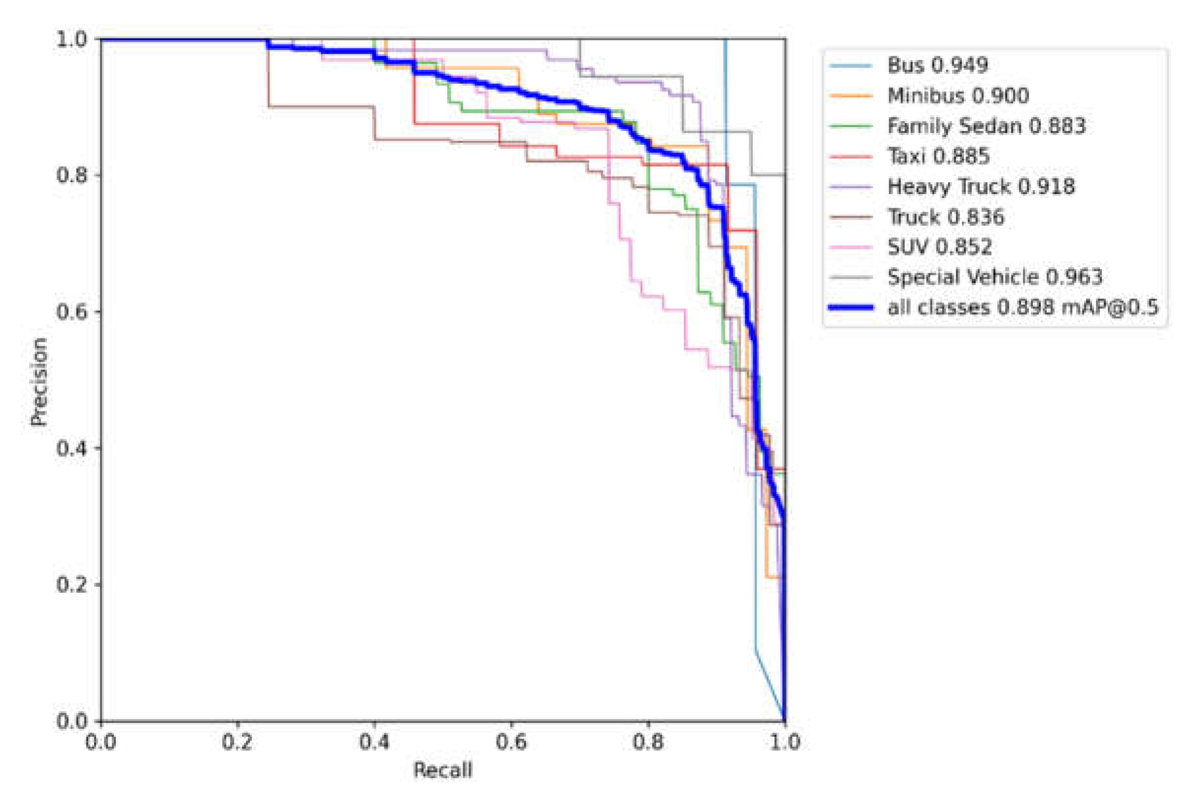
P in the PR curve [53] represents precision and R represents recall. It represented the relationship between accuracy and recall. Generally, the recall was set to abscissa and precision was set to ordinate. The results before and after algorithm improvement are shown in Figure 14 and Figure 15.
With the same hyperparameters and training rounds settings, the Mosaic method in YOLO v5 reused data while increasing the richness of the sample, and it achieved a fairly excellent performance. Both the mAP50 and mAP50:95 had been greatly improved. Compared with the original Mosaic data enhancement, the Flip-Mosaic data enhancement of YOLO v5 was more obvious in the more stringent mAP50:95. The Flip-Mosaic data enhancement performance was slightly better, which could almost eliminate the bottleneck of the limitation of the overall accuracy of the small sample category. It proved the effectiveness of the improved data enhancement optimization method in this paper.
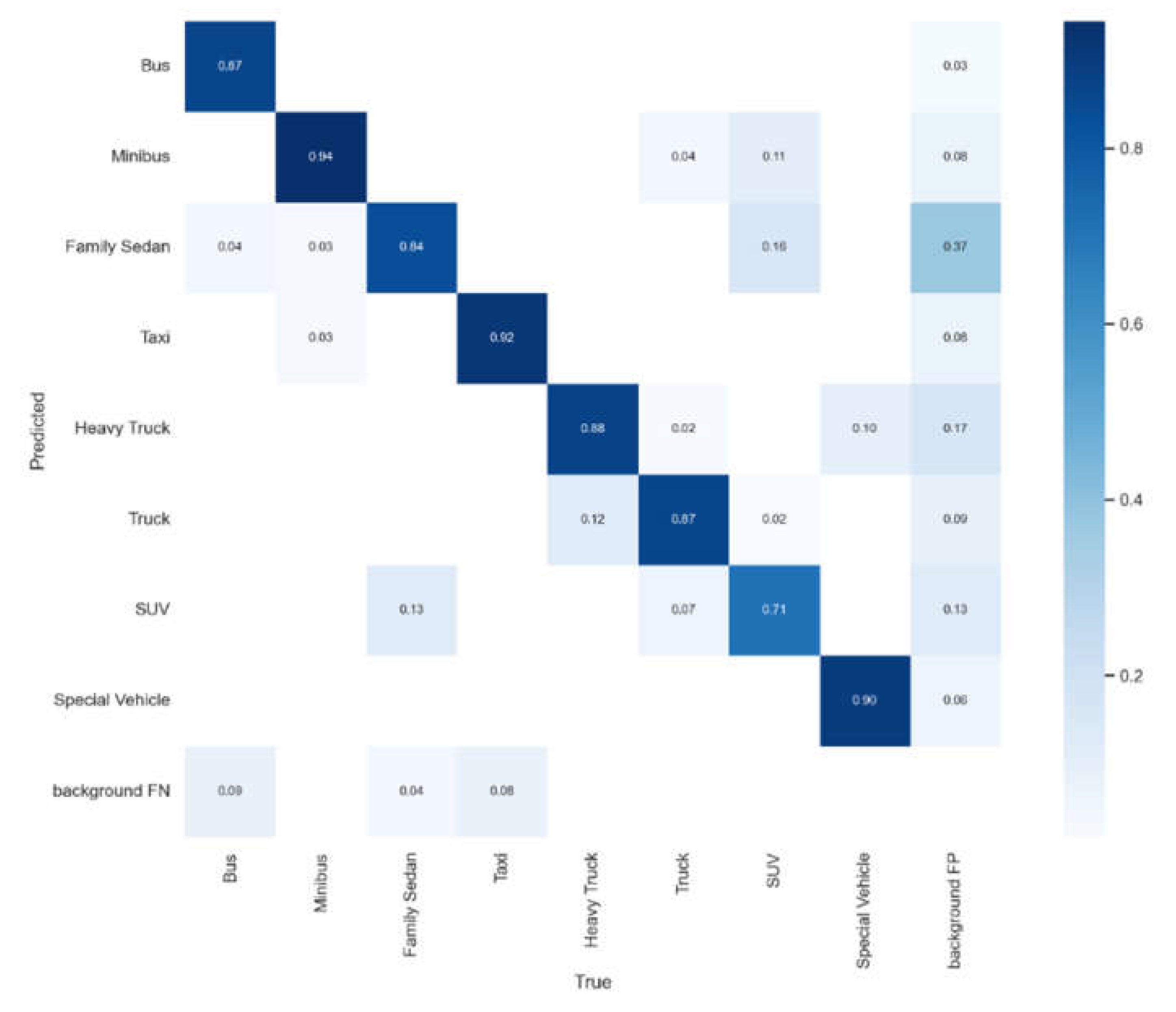
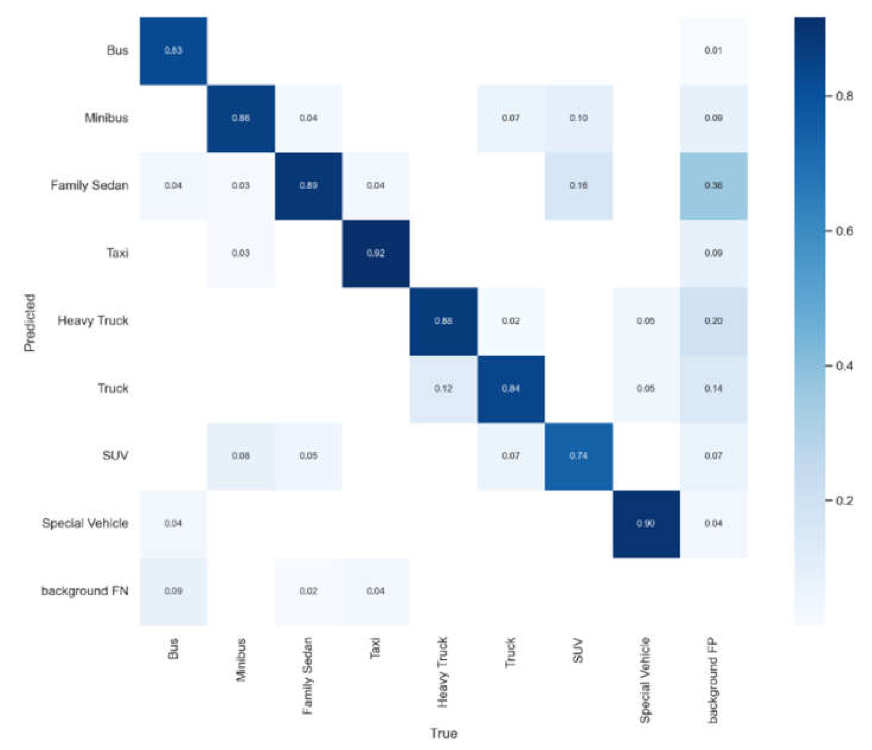
In terms of prediction, the improved YOLO v5 network shown in Figure 3, Figure 4, Figure 5, Figure 6, Figure 7, Figure 8 and Figure 9 and 3–10 had a better performance in the identification of SUVs and Family Sedans. Due to the similarity of the two models, the overall performance of the two models increased by 0.5% and 0.3%, respectively, especially in the case of a smaller calibration frame, and the overall performance was even better.
This section focused on the process of optimizing vehicle inspection performance. The principle of the YOLO v5 algorithm was introduced first. The fastest version was selected as the benchmark network. The benchmarking network was trained, and the comprehensive evaluation index of the trade-off test set, the verification set, and the small number of category indicators was designed. The evaluation results were analyzed. Then, model optimization was carried out from the data enhancement perspective. Finally, the performance before and after the improvement effect was compared, which proved the effectiveness of the improvement method proposed in this paper (Figure 16 and Figure 17).
6. Conclusions
In this paper, the high-speed scene-diversified dataset with rich data samples was constructed first. The dataset covered many scenarios of a highway, monitoring different road sections and perspectives, which provided a dataset with strong applicability for vehicle object detection in high-speed scenarios. At the same time, this article used the improved YOLO v5 network for object detection. Diverse datasets increased the accuracy of the detection of vehicle targets at the root cause. Based on this network, the Flip-Mosaic data enhancement method was studied, which significantly improved the recognition rate of similar small targets and was more in line with the requirements of engineering practice. These improvements can play a significant role in practical applications.
The traffic video intelligent monitoring system with vehicle detection designed in this paper had achieved good results in the highway scene, but there are still some problems to be improved:
- (1)
- Due to the difficulty of obtaining highway surveillance video data, the highway scene surveillance videos that could be collected in this paper were limited. More scenes, angles, and better lighting conditions of the surveillance video should be collected to further improve the generalization ability of the vehicle detection model.
- (2)
- Regarding the influence of bad weather, we need to reduce the influence of the weather environment on detection. These problems indicate that the target detection algorithm still needs to be optimized and researched.
In future autonomous driving and intelligent transportation systems, the requirements for accuracy and real-time performance will be higher. Important research directions of vehicle target detection include the dataset scene and quality problems and multi-target and small target detection problems in complex scenes, to ensure continuous optimization in order to meet higher demands.
Author Contributions
Conceptualization, Y.Z. and Z.G.; methodology, J.W. and Y.T.; validation, H.T. and X.G.; investigation, X.G.; writing—original draft preparation, X.G.; writing—review and editing, Y.T. All authors have read and agreed to the published version of the manuscript.
Funding
This research is supported by the Science and Technology Project of Shandong Provincial Department of Transportation (grant no. 2019B32) and the Key Science and Technology Projects of the Ministry of Transport of the People’s Republic of China (2019-ZD7-051). The research is partly supported by the National Nature Science Foundation of China with grant number 52002224, partly supported by the major scientific and technological innovation project of Shandong Province with grant number 2020CXGC010118, partly supported by the National Nature Science Foundation of Jiangsu Province with grant number BK20200226, and partly supported by the Program of Science and Technology of Suzhou with grant number SYG202033.
Institutional Review Board Statement
Not applicable.
Informed Consent Statement
Not applicable.
Data Availability Statement
Not applicable.
Conflicts of Interest
The authors declare no conflict of interest.
References
- Ministry of Transport of the People’s Republic of China, Statistical Bulletin of Transport Industry Development 2020. Available online: https://www.mot.gov.cn/jiaotongyaowen/202105/t20210519_3594381.html (accessed on 9 May 2022).
- Jiangsu Provincial Department of Transport, Framework Agreement on Regional Cooperation of Expressway. Available online: http://jtyst.jiangsu.gov.cn/art/2020/8/24/art_41904_9471746.html (accessed on 9 May 2022).
- Park, S.-H.; Kim, S.-M.; Ha, Y.-G. Highway traffic accident prediction using VDS big data analysis. J. Supercomput. 2016, 72, 2832. [Google Scholar] [CrossRef]
- Paragios, N.; Chen, Y.; Faugeras, O.D. Handbook of Mathematical Models in Computer Vision; Springer Science & Business Media: Berlin/Heidelberg, Germany, 2006. [Google Scholar]
- Liu, P.; Fu, H.; Ma, H. An end-to-end convolutional network for joint detecting and denoising adversarial perturbations in vehicle classification. Comput. Vis. Media 2021, 7, 217–227. [Google Scholar] [CrossRef]
- Lee, D.S. Effective Gaussian mixture learning for video background subtraction. IEEE Trans. Pattern Anal. Mach. Intell. 2005, 27, 827–832. [Google Scholar] [PubMed]
- Deng, G.; Guo, K. Self-Adaptive Background Modeling Research Based on Change Detection and Area Training. In Proceedings of the IEEE Workshop on Electronics, Computer and Applications (IWECA), Ottawa, ON, Canada, 8–9 May 2014; Volume 2, pp. 59–62. [Google Scholar]
- Muyun, W.; Guoce, H.; Xinyu, D. A New Interframe Difference Algorithm for Moving Target Detection. In Proceedings of the 2010 3rd International Congress on Image and Signal Processing, Yantai, China, 16–18 October 2010; pp. 285–289. [Google Scholar]
- Zhang, H.; Zhang, H. A Moving Target Detection Algorithm Based on Dynamic Scenes. In Proceedings of the 8th International Conference on Computer Science and Education (ICCSE), Colombo, Sri Lanka, 26–28 April 2013; pp. 995–998. [Google Scholar]
- Barnich, O.; Van Droogenbroeck, M. ViBe: A Universal Background Subtraction Algorithm for Video Sequences. IEEE Trans. Image Process. 2011, 20, 1709–1724. [Google Scholar] [CrossRef] [PubMed]
- Fang, Y.; Dai, B. An Improved Moving Target Detecting and Tracking Based On Optical Flow Technique and Kalman Filter. In Proceedings of the 4th International Conference on Computer Science and Education, Nanning, China, 25–28 July 2008; pp. 1197–1202. [Google Scholar]
- Computer Vision-ECCV 2002. In Proceedings of the 7th European Conference on Computer Vision. Proceedings, Part I (Lecture Notes in Computer Science), Copenhagen, Denmark, 28–31 May 2002; Volume 2350, pp. xxviii+817.
- Viola, P.; Jones, M. Rapid Object Detection Using a Boosted Cascade of Simple Features. In Proceedings of the 2001 IEEE Computer Society Conference on Computer Vision and Pattern Recognition. CVPR 2001, Kauai, HI, USA, 8–14 December 2001; Volume 1, p. I-511-18. [Google Scholar]
- Xu, Z.; Huang, W.; Wang, Y. Multi-class vehicle detection in surveillance video based on deep learning. J. Comput. Appl. 2019, 39, 700–705. [Google Scholar]
- Zhang, S.; Wang, X. Human Detection and Object Tracking Based on Histograms of Oriented Gradients. In Proceedings of the 9th International Conference on Natural Computation (ICNC), Shenyang, China, 23–25 July 2013; pp. 1349–1353. [Google Scholar]
- Freund, Y.; Schapire, R.E. A decision-theoretic generalization of on-line learning and an application to boosting. J. Comput. Syst. Sci. 1997, 55, 119–139. [Google Scholar] [CrossRef]
- Yu, K. A least squares support vector machine classifier for information retrieval. J. Converg. Inf. Technol. 2013, 8, 177–183. [Google Scholar]
- Felzenszwalb, P.; McAllester, D.; Ramanan, D. A discriminatively trained, multiscale, deformable part model. In Proceedings of the IEEE Conference on Computer Vision and Pattern Recognition, Anchorage, Alaska, 23–28 June 2008; p. 1984. [Google Scholar]
- He, N.; Zhang, P.-P. Moving Target Detection and Tracking in Video Monitoring System. Microcomput. Inf. 2010, 3, 229–230. [Google Scholar]
- Wu, X.; Song, X.; Gao, S.; Chen, C. Review of target detection algorithms based on deep learning. Transducer Microsyst. Technol. 2021, 40, 4–7+18. [Google Scholar]
- Xie, W.; Zhu, D.; Tong, X. Small target detection method based on visual attention. Comput. Eng. Appl. 2013, 49, 125–128. [Google Scholar]
- Girshick, R.; Donahue, J.; Darrell, T.; Malik, J. Rich feature hierarchies for accurate object detection and semantic segmentation. In Proceedings of the 27th IEEE Conference on Computer Vision and Pattern Recognition (CVPR), Columbus, OH, USA, 23–28 June 2014; pp. 580–587. [Google Scholar]
- He, K.; Zhang, X.; Ren, S.; Sun, J. Spatial Pyramid Pooling in Deep Convolutional Networks for Visual Recognition. In Proceedings of the 13th European Conference on Computer Vision (ECCV), Zurich, Switzerland, 6–12 September 2014; pp. 346–361. [Google Scholar]
- Girshick, R. Fast r-cnn. In Proceedings of the Tenth IEEE International Conference on Computer Vision, Beijing, China, 17–20 October 2005; pp. 1440–1448. [Google Scholar]
- Zheng, X.; Chen, F.; Lou, L.; Cheng, P.; Huang, Y. Real-Time Detection of Full-Scale Forest Fire Smoke Based on Deep Convolution Neural Network. Remote Sens. 2022, 14, 536. [Google Scholar] [CrossRef]
- Zhao, H.; Li, Z.; Zhang, T. Attention Based Single Shot Multibox Detector. J. Electron. Inf. Technol. 2021, 43, 2096–2104. [Google Scholar]
- Redmon, J.; Divvala, S.; Girshick, R.; Farhadi, A. You Only Look Once: Unified, Real-Time Object Detection. In Proceedings of the 2016 IEEE Conference on Computer Vision and Pattern Recognition (CVPR), Seattle, WA, USA, 27–30 June 2016; pp. 779–788. [Google Scholar]
- Redmon, J.; Farhadi, A. YOLO9000: Better, faster, stronger. arXiv 2016, arXiv:1612.08242. [Google Scholar]
- Li, J.; Huang, S. YOLOv3 Based Object Tracking Method. Electron. Opt. Control 2019, 26, 87–93. [Google Scholar]
- Bochkovskiy, A.; Chien-Yao, W.; Liao, H.Y.M. YOLOv4: Optimal speed and accuracy of object detection. arXiv 2020, arXiv:2004.10934. [Google Scholar]
- Zhan, W.; Sun, C.; Wang, M.; She, J.; Zhang, Y.; Zhang, Z.; Sun, Y. An improved Yolov5 real-time detection method for small objects captured by UAV. Soft Comput. 2022, 26, 361–373. [Google Scholar] [CrossRef]
- St-Aubin, P.; Miranda-Moreno, L.; Saunier, N. An automated surrogate safety analysis at protected highway ramps using cross-sectional and before-after video data. Transp. Res. Part C Emerg. Technol. 2013, 36, 284–295. [Google Scholar] [CrossRef]
- Dong, Z.; Wu, Y.; Pei, M.; Jia, Y. Vehicle Type Classification Using a Semisupervised Convolutional Neural Network. Ieee Trans. Intell. Transp. Syst. 2015, 16, 2247–2256. [Google Scholar] [CrossRef]
- Manzano, C.; Meneses, C.; Leger, P. An Empirical Comparison of Supervised Algorithms for Ransomware Identification on Network Traffic. In Proceedings of the 2020 39th International Conference of the Chilean Computer Science Society (SCCC), Coquimbo, Chile, 16–20 November 2020; p. 7. [Google Scholar]
- Razakarivony, S.; Jurie, F. Vehicle detection in aerial imagery: A small target detection benchmark. J. Vis. Commun. Image Represent. 2016, 34, 187–203. [Google Scholar] [CrossRef] [Green Version]
- Lin, T.-Y.; Maire, M.; Belongie, S.; Hays, J.; Perona, P.; Ramanan, D.; Dollar, P.; Zitnick, C.L. Microsoft COCO: Common Objects in Context. In Proceedings of the 13th European Conference on Computer Vision (ECCV), Zurich, Switzerland, 6–12 September 2014; pp. 740–755. [Google Scholar]
- de Haan, K.; Rivenson, Y.; Wu, Y.; Ozcan, A. Deep-Learning-Based Image Reconstruction and Enhancement in Optical Microscopy. Proc. IEEE 2020, 108, 30–50. [Google Scholar] [CrossRef]
- Shorten, C.; Khoshgoftaar, T.M. A survey on Image Data Augmentation for Deep Learning. J. Big Data 2019, 6, 60. [Google Scholar] [CrossRef]
- Casteleiro, M.A.; Demetriou, G.; Read, W.; Prieto, M.J.F.; Maroto, N.; Fernandez, D.M.; Nenadic, G.; Klein, J.; Keane, J.; Stevens, R. Deep learning meets ontologies: Experiments to anchor the cardiovascular disease ontology in the biomedical literature. J. Biomed. Semant. 2018, 9, 13. [Google Scholar] [CrossRef]
- Yang, S.J.; Berndl, M.; Ando, D.M.; Barch, M.; Narayanaswamy, A.; Christiansen, E.; Hoyer, S.; Roat, C.; Hung, J.; Rueden, C.T.; et al. Assessing microscope image focus quality with deep learning. BMC Bioinform. 2018, 19, 77. [Google Scholar] [CrossRef]
- Guo, Y.; Zeng, Y.; Gao, F.; Qiu, Y.; Zhou, X.; Zhong, L.; Zhan, C. Improved YOLOV4-CSP Algorithm for Detection of Bamboo Surface Sliver Defects With Extreme Aspect Ratio. IEEE Access 2022, 10, 29810–29820. [Google Scholar] [CrossRef]
- Yinpeng, C.; Xiyang, D.; Mengchen, L.; Dongdong, C.; Lu, Y.; Zicheng, L. Dynamic Convolution: Attention over Convolution Kernels. In Proceedings of the IEEE/CVF Conference on Computer Vision and Pattern Recognition (CVPR), Seattle, WA, USA, 14–19 June 2020; pp. 11027–11036. [Google Scholar]
- Kaixin, W.; Jun Hao, L.; Yingtian, Z.; Daquan, Z.; Jiashi, F. PANet: Few-shot image semantic segmentation with prototype alignment. In Proceedings of the IEEE/CVF International Conference on Computer Vision (ICCV), Seoul, Korea, 27 October–2 November 2019; pp. 9196–9205. [Google Scholar]
- Simon, M.; Milz, S.; Amende, K.; Gross, H.-M. Complex-YOLO: An Euler-Region-Proposal for Real-Time 3D Object Detection on Point Clouds. In Proceedings of the 15th European Conference on Computer Vision (ECCV), Munich, Germany, 8–14 September 2018; pp. 197–209. [Google Scholar]
- Wenqiang, X.; Haiyang, W.; Fubo, Q.; Cewu, L. Explicit Shape Encoding for Real-Time Instance Segmentation. In Proceedings of the IEEE/CVF International Conference on Computer Vision (ICCV), Seoul, Korea, 27 October–2 November 2019; pp. 5167–5176. [Google Scholar]
- Huang, Z.; Wang, J. DC-SPP-YOLO: Dense connection and spatial pyramid pooling based YOLO for object detection. Inf. Sci. 2020, 522, 241–258. [Google Scholar] [CrossRef]
- Zhaohui, Z.; Ping, W.; Wei, L.; Jinze, L.; Rongguang, Y.; Dongwei, R. Distance-IoU loss: Faster and better learning for bounding box regression. Proc. AAAI Conf. Artif. Intell. 2019, 34, 12993–13000. [Google Scholar]
- Hendry; Chen, R.-C. Automatic License Plate Recognition via sliding-window darknet-YOLO deep learning. Image Vis. Comput. 2019, 87, 47–56. [Google Scholar] [CrossRef]
- Gao, J.; Chen, Y.; Wei, Y.; Li, J. Detection of Specific Building in Remote Sensing Images Using a Novel YOLO-S-CIOU Model. Case: Gas Station Identification. Sensors 2021, 21, 1375. [Google Scholar] [CrossRef]
- Yang, S.-D.; Zhao, Y.-Q.; Yang, Z.; Wang, Y.-J.; Zhang, F.; Yu, L.-L.; Wen, X.-B. Target organ non-rigid registration on abdominal CT images via deep-learning based detection. Biomed. Signal Process. Control 2021, 70, 102976. [Google Scholar] [CrossRef]
- Du, J. Understanding of Object Detection Based on CNN Family and YOLO. In Proceedings of the 2nd International Conference on Machine Vision and Information Technology (CMVIT), Hong Kong, China, 23–25 February 2018. [Google Scholar]
- Huang, R.; Pedoeem, J.; Chen, C. YOLO-LITE: A Real-Time Object Detection Algorithm Optimized for Non-GPU Computers. In Proceedings of the IEEE International Conference on Big Data (Big Data), Seattle, WA, USA, 10–13 December 2018; pp. 2503–2510. [Google Scholar]
- Hou, Q.; Cheng, M.-M.; Hu, X.; Borji, A.; Tu, Z.; Torr, P.H.S. Deeply Supervised Salient Object Detection with Short Connections. IEEE Trans. Pattern Anal. Mach. Intell. 2019, 41, 815–828. [Google Scholar] [CrossRef] [Green Version]
Figure 1.
The sampling location of different surveillance scenario videos.

Figure 2.
Examples of different scene datasets.

Figure 3.
Schematic diagram of vehicle sample classification in dataset.

Figure 4.
The flowchart of image data annotation processing.

Figure 5.
Schematic diagram of rectangular box label.

Figure 6.
Schematic diagram of vehicle occlusion.

Figure 7.
Statistical chart of labeling information.

Figure 8.
Distribution proportion.

Figure 9.
Network structure of YOLO v5.

Figure 10.
Processing flow of Focus module.

Figure 11.
Decoding of prediction bounding box in YOLO v5.

Figure 12.
The data augmentation algorithm of traditional Mosaic.

Figure 13.
The data augmentation algorithm of Flip-Mosaic.

Figure 14.
Standard YOLO v5 PR curve.

Figure 15.
Improved YOLO v5 PR curve.

Figure 16.
Recognition accuracy of standard YOLO v5 network.

Figure 17.
Recognition accuracy of improved YOLO v5 network.


Table 1.
Schematic diagram of txt annotated text file.
| Category | x | y | w | h |
|---|---|---|---|---|
| 4 | 0.837022 | 0.602114 | 0.274942 | 0.499098 |
| 4 | 0.303379 | 0.385564 | 0.140371 | 0.243362 |
| 2 | 0.558019 | 0.140139 | 0.023202 | 0.037123 |
Table 2.
Annotation category information of YOLO.
| Annotation Category Information of YOLO | |||
|---|---|---|---|
| Bus | 0 | Heavy Truck | 4 |
| Minibus | 1 | Truck | 5 |
| Family Sedan | 2 | SUV | 6 |
| Taxi | 3 | Special Vehicle | 7 |
Publisher’s Note: MDPI stays neutral with regard to jurisdictional claims in published maps and institutional affiliations. |
© 2022 by the authors. Licensee MDPI, Basel, Switzerland. This article is an open access article distributed under the terms and conditions of the Creative Commons Attribution (CC BY) license (https://creativecommons.org/licenses/by/4.0/).
Share and Cite
MDPI and ACS Style
Zhang, Y.; Guo, Z.; Wu, J.; Tian, Y.; Tang, H.; Guo, X. Real-Time Vehicle Detection Based on Improved YOLO v5. Sustainability 2022, 14, 12274. https://doi.org/10.3390/su141912274
AMA Style
Zhang Y, Guo Z, Wu J, Tian Y, Tang H, Guo X. Real-Time Vehicle Detection Based on Improved YOLO v5. Sustainability. 2022; 14(19):12274. https://doi.org/10.3390/su141912274
Chicago/Turabian StyleZhang, Yu, Zhongyin Guo, Jianqing Wu, Yuan Tian, Haotian Tang, and Xinming Guo. 2022. "Real-Time Vehicle Detection Based on Improved YOLO v5" Sustainability 14, no. 19: 12274. https://doi.org/10.3390/su141912274
Note that from the first issue of 2016, this journal uses article numbers instead of page numbers. See further details here.