


3D-Printable Materials Made with Industrial By-Products: Formulation, Fresh and Hardened Properties


Laboratoire de Génie Civil et géo-Environnement (LGCgE), ULR 4515, University of Lille, Junia, IMT Nord Europe, University of Artois, 62400 Béthune, France
*
Author to whom correspondence should be addressed.
Sustainability 2022, 14(21), 14236; https://doi.org/10.3390/su142114236
Submission received: 5 October 2022
/
Revised: 22 October 2022
/
Accepted: 24 October 2022
/
Published: 31 October 2022
(This article belongs to the Special Issue Sustainable Civil Engineering Structures and Construction Materials)
Abstract
:Growing in the field of construction, 3D printing allows to build non-standard shapes and to optimise the use of resources. The development of printable materials requires good control of the fresh state of the material—between mixing and printing, a printable material has to evolve from fluid matter to be pumpable (extrudability) up to a matter supporting its own weight and those of superior layers (buildability). Our researches are focused on printable materials used in large printers, i.e., printers able to build structural pieces for buildings. As many pumps and printers can be used to achieve a wide range of parts, this paper presents a simple method to provide valuable guidance to users when a decision needs to be made about printable materials. In this context, our researches both try to maximise the use of industrial by-products to reduce the environmental cost of printed material and to propose tests easy to carry out in the field. Consequently, on the one hand, some printable materials that mainly include quarry washing fines have been developed and, on the other hand, Fall cone and Vicat tests have been used to determine the printability limit. By not focusing on a single formula, the novelty of this paper is to present to readers some parametric models, i.e., a methodology that can be used according to their own devices and applications. Based on a design of experiments, 20 formulas have been tested. Parameters that influence the quality of printing are highlighted. Mechanical tests results at hardened state and shrinkage measurements are also shown to demonstrate the ability of some formulas to be structural materials: compressive strengths at 28 days between 7.50 MPa and 18.40 MPa.
1. Introduction
1.1. Context
In the last decades, the development of computing sciences has led to the emergence of innovative automated processes such as additive manufacturing (AM), also known as 3D-printing. Elements are produced layer upon layer thanks to 3D models which were previously created with a CAD software [1,2]. Implementation of additive manufacturing (AM) in the construction industry has now been studied for more than 20 years and many technologies have already been designed to manufacture either construction elements or entire buildings [3,4,5]. Additionally, AM allows for a higher geometry complexity level than formwork techniques. Hager et al. as well as De Schutter et al. highlight the advantages of introducing AM in the building industry, such as lowering the production costs, the need for resources and the amount of generated wastes, but materials optimisation remains a great challenge [6,7]. Even though sand concrete is still the most used material, interest in alternative resources, such as earthen materials, is growing nowadays [8,9]. Indeed, raw earth has been a traditional construction material for millennia all over the world and involves few logistic requirements as its ubiquity enables it to be extracted near the construction site [10,11]. As suggested by Sauerwein et al., local materials have to be privileged for enhancing the building inks sustainability and for participating in the reduction of the environmental impact of building materials [12]. Earthen materials (from earthwork, for example) or industrial by-products can be considered as local materials and are interesting alternative resources for mix designs of 3D printing materials [13,14].
Mortar-extrusion-based processes are the most studied in the field of construction, such as Contour Crafting, for entire building manufacturing, or Concrete Printing, suitable for smaller elements [15,16,17,18]. Even though the process only requires a concrete pump to feed the AM device, the material kinetics must be taken into account to prevent it from setting into the system and damaging it. Le et al. highlighted the need to find a rheological compromise so that the feeding material would be fluid enough to be pumped and extruded through the printer nozzle (Extrudability), but it also has to be stiff enough to maintain its shape without noticeable deformation under the pressure of its own weight and those of the upper layers (Buildability) [19,20,21]. Considering that these materials exhibit a Bingham-fluid-like behaviour, their consistency evolution could be monitored by measuring their static yield stress () with a rheometer [15,22,23,24]. Indeed, Roussel brought to light existing relations between and 3D-printing parameters, such as printed height, material density, and deposition speed [25]. Moreover, penetration tests are useful for quick consistency measurements and have proven to be efficient in estimation with fast-setting materials [26,27,28].
Kazemian et al. and Lu et al. have both proposed step-by-step procedures to develop 3D-printable materials (3DPMs) [15,29]. However, this kind of methodology would require to restart trials from the previous step whenever the material does not comply with its specifications. Jiao et al. emphasize the advantages of introducing design of experiments (DoE) into concrete formulation methodology to reduce the number of experiments [30]. Among the great variety of existing DoE, simplex centroid design or Taguchi’s array have already been applied [30,31,32]. Moreover, as outlined by Wangler et al., 3D printing of cementitious materials could be regarded as complex chemical processes which are often studied with DoE methodology for robustness or optimisation purposes [33,34].
1.2. Objectives
This research work aims to formulate printable materials that include a large amount of industrial by-products and are stabilised with various proportions of cement blends. As the combination of mixing components allows to create a wide variety of formulas, the DoE seems to be a suitable method to analyse parameters’ influence with a small number of formulas. In this paper, 20 formulas are developed and their fresh state properties are studied in order to produce feature forecasts. Another important point is that the existence of various printing devices and printed parts prevents us from providing a single formula that can be applied in all cases. Therefore, our objectives are to create models that both estimate the initial setting time to know if the material has lost its plasticity and can be extruded and the printability limit to know if the material can retain its mechanical properties during printing process. Then, influences of mixing components (quarry fines, ordinary portland cement, cement mix, calcium sulfoaluminate cement, fly ashes, citric acid monohydrate and water) have to be determined. Thanks to an unconventional DoE and mechanical tests (Fall Cone Penetrometer), the main parameters have been identified and a predictive model with a good accuracy is proposed. According to their printing device, the users could identify the most suitable formula for their applications. Finally, some tests at hardened state show the capacity of studied mixes to respond to various types of applications.
2. Materials and Methods
2.1. Materials
Calcareous quarry fines (QF), from Ferques (FR62250), were chosen as the main component. These QF are by-products from the extracted aggregates washing step. The chosen quarry is one of largest quarries in France. Their activities induce 300,000 tons of washing fines. Currently, several million tons are stored in solid or liquid state and represent an interesting alternative to local materials with a high potential of use in civil engineering for the North of France. These fines are mainly composed of limestone (62% w/w) with other minerals (11% w/w quartz, 5% w/w dolomite, 3% w/w goethite) and a low amount of clays (12% w/w kaolinite and 7% w/w illite) [35]. Particle size ranges from 0.1 to 100 µm, the specific gravity is 2650 and the bulk density—1860 . The liquid limit was determined to be 33% and the Plastic index—12% [36]. Loss on drying performed at 105 °C during 24 h remained stable at 0.8% (w/w) for storage relative humidity from 40% to 70%. These quarry washing fines have a similar behaviour to silt or low-plastic clay according to French standard NF P 11-300 [37].
The hydraulic binders used in this study are blends of ordinary Portland Cement (OPC) CEM I 52.5 R CE CP2 NF from Couvrot (FR51300), calcium sulfoaluminate cement (CSAC) ALPENAT R from Saint Egrève (FR38120) and biomass boilers fly ashes (FA) from Gardanne (FR13120). The materials’ chemical composition as well as their main characteristics are summarized in Table 1. Due to its effectiveness in regulating CSAC setting rate, citric acid was chosen to be the setting retarder [38]. Citric acid monohydrate (CAM), supplied by BFC SAS from Rémalard-en-Perche (FR61110), was previously crushed and sieved at 250 µm before use. Fresh mixes were produced using tap water.
2.2. Mix Design
2.2.1. Formulation Methodology
The 3DPMs manufacturing process is displayed in Figure 1. For every experiment, a dry mix (HB) was formulated by blending an hydraulic binder (HB) with QF. HBs were obtained combining a cement mix (CM) (OPC and CSAC blend) with FA. CAM was then dispersed into the DM. The mixer was started just before pouring the water, the amount of which has to be adjusted for the material to achieve the targeted consistency. According to the mix methodology and a previous bibliographic review, among many possible influencing factors, four seem to be very relevant to investigate:
- Hydraulic binder weight ratio in the dray mix (P1);
- Citric acid monohydrate amount added to the dry (P2);
- Ordinary portland cement weight ratio in the cement blend (P3);
- Fly ash content in the hydraulic binder (P4).
Once the study parameters are selected, suitable levels and a DoE have to be established.
2.2.2. Design of Experiments
The choice was made to analyse these four parameters’ impact with a limited number of 20 different formulas. An unconventional design, obtained by removing the 5th column of a Taguchi array and adding 4 more rows to improve information (Appendix A), was preferred to full factorial matrices [39,40]. One of the additional trials corresponds to the experimental domain centre (E17). The others focus on parameters P1 (quantity of binder) and P3 (nature of the cement mixture), which are suspected to have the strongest influence on 3DPMs properties. In the first instance, studied levels were defined (Table 2), then, applying the DoE, a mix design was shaped (Table 3).
Extrusion-based AM techniques require a high cement content so P1 was set to be at least 25% but no more than 50% to obtain a dry mix with at least 50% of by-products QF and FA) [15,16,19,41]. A P2 minimal value of 0.4% weight ratio was necessary to attain at least 30 min of workability with the fastest mix and maximum level was set to 1.0% to prevent materials from setting too slowly. P3 focuses on the nature of the CM used to formulate the HB (OPC, CSAC or a mix of both). Afterwards, mineral substitution in the binder with FA (P4) was set to the range from 0.0% to 24.0% (maximal value permitted by French standard NF EN 450-1 [42]).
2.3. Mixing Procedure
Careful consideration was given to experimental conditions to prevent temperature variability from impacting the manufacturing process. All materials were stored at 20 C ± 1 C before being used. The mixing procedure is the following one:
- 1.
- QF, OPC, CSAC and FA are weighed and poured into a planetary mixer;
- 2.
- CAM is added to the DM and dispersed for about 1 min at low speed;
- 3.
- At , tap water is poured into the mixer for 30 s to 1 min at low speed;
- 4.
- At 1 min, blending speed is raised up to high speed for 2 min;
- 5.
- At 3 min, mixer is stopped to scrap the bowl and blades;
- 6.
- Mixing is started again for 2 min more at high speed;
- 7.
- Mixing is stopped and the material is gathered into a ball;
- 8.
- At 15 min, the 3DPMs consistency is checked.
In this case, low speed is set at 60 revolutions/min and 140 rotations/min and high speed is set at 120 revolutions/min and 280 rotations/min.
If the material consistency complies with the acceptance criteria (Extrudability and Buildability), it will be considered suitable for the printing process. Otherwise, the amount of water must be adjusted first to reach the suitable starting consistency. In this case, an appropriate method for consistency measurements has to be introduced.
3. Characterisation Tests
3.1. Water Dosage and Bulk Density
3.1.1. Experimental Background
During background trials in the course of the research project MATRICE, a fall cone penetrometer (Figure 2) was found to be adequate in consistency checking and a fall cone penetration depth (FCPD) between 16 and 20 mm at the start of the printing session was found to be adequate to be both extrudable and buildable [43]. In fact, according to Koumoto et al., this range matches the Atterberg Liquid Limit, also defined as the beginning of soils plastic domain [44]. This limit is 17 mm FCPD in French standard NF P94-052-1 and 20 mm in British standard BS 1377-2 [45] and in NF EN ISO 17892-12 [46], both using a 80 g metal cone with a 30° angle. As the 3DPMs manufacturing process lasted from 10 to 15 min during full-scale printing sessions, a targeted value of 18.0 mm depth of penetration at + 15 min (), with a 2.0 mm tolerated deviation (16.0 mm ≤≤ 20.0 mm), was adopted as our acceptance criterion.
3.1.2. Measurements
The fall cone penetrometer was chosen for water assays too as its response could be considered as being linear with our earthen material in the range from 10 to 25 mm FCPD. Fall cone linearity was also demonstrated on kaolin pastes by Perrot et al. [47]. For each DM, FCPD were performed with 3 different water-to-dry-mix weight ratio (WDM) surrounding the targeted value (18.0 mm). For each WDM, 3 measures of were recorded according to NF EN ISO 17892-12 [46]. Mean values and standard deviations were calculated, then linear regression was performed on the mean values. The computed functions allowed us to easily estimate the optimal WDM () to achieve our target consistency. Fresh mixes were composed with their respective , then their bulk densities were measured by weighting a 1000 mL sample. The density were also determined for two modulations of formula E17 with WDM to reach 16 mm and WDM to reach 20 mm penetration depth WDM to reach 20 mm penetration depth (), respectively on E17 and E17.
3.2. Setting Kinetics
3.2.1. Initial Setting Time
Initial setting time (IST) was determined thanks to a Vicat automated apparatus compliant with [NF EN 480-2] [48]. Measures were recorded every 10 min and as soon as the distance separating the edge of the needle and the rubber plate beneath the specimen mould reaches a value between 3 to 6 mm, the material is considered as having attained its IST. However, as outlined by Kazemian et al., IST is longer than the end of workability, but it is also longer than the Blocking Limit, defined as the time for the 3DPMs to be too stiff to be extruded through the pumping system, which could lead to dire consequences [29]. For this reason, even though IST could give us an indication of the setting kinetics, it is not relevant enough to be considered alone. Another suitable time must be defined to identify the end of workability.
3.2.2. Workability
The fall cone penetrometer also proved to be appropriate in consistency evolution monitoring and identifying a suitable time to determine the end of workability. Indeed, as soon as the FCPD fell below 10 mm, most of our formulations displayed visible cracks on their surface just after sample preparation (Figure 3). Kazemian et al. also defined a printability limit (Prim Lim) as the time when the extruded material does not comply with its printing quality expectations any longer [29]. In the same spirit, this FCPD value of 10 mm was identified in this study as the end of workability.
Fall cone trials were carried out, performing 3 measurements at each following timeline:
- 1.
- 10/15/20/25/30/35/40/45/50/55/60 min
- 2.)
- 70/80/90/100/110/120 min
- 3.
- 135/150/165/180/195/210/225/240 min
- 4.
- 260/280/300/320/340/360 min
- 5.
- 390/420/450/480/510/540/570/600 min
where is the time when water was added and t the time when measures were performed, and none of the formulas’ Print Lim was more than 600 min.
Tests were stopped when the FCPD fell below 10 mm. The corresponding time was reported as the Print Lim. According to our printing sessions feedback, an open time longer than 60 min and shorter than 180 min was targeted with our experimental conditions. Another range could be preferred depending on the AM device and the printing parameters.
3.2.3. Yield Stress Estimation
Some 3DPMs exhibit very rapid setting rates, making rheological measurements quite difficult with a shear vane apparatus. Therefore, static yield stress was estimated with a quick penetration test, such as Lootens et al., but using the fall cone instead of a cylindrical device [26]. Applying the cone geometry to the Lootens pattern, we could deduce as a function of the FCPD:
where is the static yield stress in Pa, g is the gravitational force equivalent (9.81 N·kg), the depth of penetration in mm, m is the cone mass in kg and —its angle (0.080 kg and for the British cone).
In the course of preparatory works on QF mixes, Equation (1) gave us an overestimation of compared to values observed with a shear vane apparatus following the same procedure as Perrot et al. [24]. Indeed, the theoretical value of 2.3 kPa at 20 mm FCPD is higher than the obtained 1.9 kPa value. Geotechnical literature generally relies on the Hansbo model (Equation (2)) to estimate undrained shear strength around soils’ liquid limit [44]:
where is the static yield stress in Pa, is the undrained shear strength in Pa, K is the cone correction factor, F the cone weight force in N, m—its mass in kg, g is the g-force and the depth of penetration in m.
Although the fall cone used in this study according to BS 1377-2 [45] has a constant factor K reported to be 0.74, a 1.5 kPa shear strength is normally expected when FCPD is 20 mm, but observations vary between 0.7 and 3 kPa from one research work to another, depending more on the material nature than the selected cone [44,49,50,51]. Assuming the equivalence between and undrained shear strength , the theoretical K factor for Lootens model (Equation (1)) was calculated to be 1.15, but it was found to be 0.97 in our case during preliminary tests with QF. Supposing K factor which was calculated to be in accordance with our earthen material remains the same whatever the DoE formula, then could be more accurately estimated by correcting Equation (1) with the K factors ratio:
where is the static yield stress in Pa, 0.97 is the K value found with QF preliminary tests, 1.15 is the theoretical K value for Lootens model equivalence and the fall cone depth of penetration in mm.
Equation (3), in line with our earthen material, was adopted to estimate evolution.
3.3. Main Effects Analysis
For this research work, only first-order models based on either parameters or dry ingredients were computed. Thus, water dosage impact as well as parameter or component interactions are not investigated in this paper.
3.3.1. Composition and Response Relations
DoEs allow to generate predictive models, but, even though our parameters were chosen according to a bibliographic review, strong links between them exist (Table 4), which could lead to skewed modelling. With this in mind, two models were explored instead of one. The first model was called Parametric and it generates a predictive model thanks to the DoE (Appendix A) and its selected levels (Table 2). The second one was called the Component model and it relies on mix ingredient contents (Table 3) such as mixture designs [31,52]. Assuming a first-order linear model, each response (where n is the experiment number) could be expressed respectively by either Equation (4a) (Parametric) or (4b) (Component).
where n is the experiment number and its measured response, i is the parameter number, p the total count of parameters, the corresponding level of parameter i in formula En, —the effect of parameter i, corresponds to the Mean Effect, j—the component number, q—the overall number of components, —the weighting coefficient of component j and is the component to DM weight ratio in formula En.
The matrices used to compute our models are presented in Appendix B.1, Appendix B.2 and Appendix B.3. To simplify calculations, we admitted that the total DM mass, in the Component model, is the sum of OPC, CSAC, FA and QF for the reason that CAM ratio values in all mixes are less than 1.0%.
3.3.2. Effects Calculation and Quick Data Analysis
Our first-order models were computed according to Equations (5a) (parametric) and (5b) (component) [39,52]:
where Y is the responses matrix, X and X are, respectively, the parametric and component matrices, B and C—the parametric and component effects matrices (see Appendix B.1, Appendix B.2 and Appendix B.3).
The assessment of B and C could provide a synthetic analysis of parameters and components influence on the different responses. Nevertheless, as mentioned above, modelling bias could lead to poor forecasting quality, especially if strong interactions exist. The normalised root square deviation (NRMSD) was selected along with the coefficient of determination () to conduct a quick investigation on our models’ predictive quality [34,53]:
where is the root mean square deviation estimator, N—the total number of experiments, —the mean of recorded responses and are the predicted response.
RMSD estimates the average error between predicted and observed values. It is analogous to Standard Deviation (SD) used in process engineering for robustness analyses [52]. As a relative value, NRMSD, the RMSD-to-response mean ratio, was preferred for fast comparison. The closer this value is to zero, the better the predictive quality.
3.4. Hardened Properties
To identify the potential use ways of studied mixes, some tests were conducted in the hardened state.
3.4.1. Mechanical Performances
Compressive tests were performed on four cast cubic specimens (40 × 40 × 40 mm per formula, with an automated electromechanic press of 50 kN force capacity (precision level: ±0.5% from 0.0 to 0.5 kN then ± 0.3% from 0.5 kN to 50 kN). Two curing times were chosen: 24 h and 28 days. Due to the lack of standard in additive-manufactured products, a load velocity of 5 for compressive tests, such as the one used by Dubois et al. [35], was chosen to ensure a satisfying load distribution into the samples. Every sample was unmoulded at + 23 h and then stored in a climatic room (20 C/50% HR), to reproduce air drying conditions.
3.4.2. Shrinkage
Specimen preparation was performed according to the NF EN 12390-16 [54]. The shrinkage mould length was measured with a 0.1 mm precision caliper and reported as the sample initial length ().
For each formula, two prismatic samples of 40 × 40 × 160 dimension were produced. After being unmoulded at + 48 h, every sample was stored in a climatic room at ambient conditions (20 °C/50% HR) to reproduce air-drying conditions and their length (L) were recorded at 7, 28 and 180 days with a 0.01 mm precision electronic caliper. Hence, dimensional variation could be expressed as:
here is the dimensional variation in , L the sample length recorded in mm and is the initial length in mm.
4. Results and Discussion
All data calculations were performed using open-source numerical computation software Scilab (6.0.2) [55].
4.1. Mixing Water and Bulk Density
The mean values of recorded , the standard deviations and linear regression functions of formulas E10, E14 and E17 are outlined in Figure 4. E17 is the experimental domain centre, whereas E10 and E14 are, respectively, the least and most water sensitive formulas. On the basis of our results, all of them are highly sensitive to water; this is why WDM had to be determined with at least a 0.1% accuracy level. Each linear slope was defined as a water sensitivity coefficient (WSC) to assess water influence on the materials’ consistency. Indeed, E14 WSC is 3.00 which indicates that a 1% increase of WDM will add 3.00 mm to the FCPD, for instance, whereas it would only be 1.55 mm with formula E10 (WSC is 1.55). Once all , WDM had reached 16 mm penetration depths () and werecalculated, bulk densities were measured weighting a 1000 mL sample of fresh mixes composed with their respective . The results are reported in Table 5.
Over the whole DoE, varies from 28.8% (E20) to 35.9% (E4), which are values close to the QF liquid limit (33%), suggesting that 3DPMs are heavily influenced by QF nature.
Further investigations with other earthen materials would be necessary to confirm this. WSC-impacting factors are very difficult to evaluate directly and the results would require effects matrices computation first. Comparing E17 and E17 densities shows that WDM has a meaningless impact within its tolerable variation range.
4.2. Setting Kinetics
4.2.1. Printability Limits and Initial Setting Times
The 3DPMs were classified in 3 different categories: the fast-setting formulas, (Print Lim ≤ 90 min), the slow-setting ones (Print Lim ≥ 240 min) and the moderate-setting formulations for Print Lim between 90 min and 240 min (Table 6). Recorded data and curves exhibit very different profiles, so, as it is difficult to compare all formulations together, focus was placed on five different ones: E4 and E7 (slow setting), E14 and E19 (rapid setting) and E17 (centre of the DoE with a moderate setting rate). As soon as FCPDs curves cross the 10 mm limit, corresponding times (pointed by label arrows in Figure 5) are reported as the Print Lim. ISTs were recorded, then IST-to-Print Lim ratios were calculated for every formula. All results are displayed in Table 6.
Comparing E1 and E19 (pure CSAC binder) with E18 and E20 (pure OPC binder), both Print Lim and IST appear to be highly influenced by the cement nature (P3), much more than its content (P1). Particular attention was given to E14 as its Vicat measures showed a very rapid setting rate just after reaching its IST. Indeed, recorded values were 0.0 mm at 130 min, 5.5 at 140 min, 25.3 at 150 min, 38.6 at 160 min and then 39.6 after 180 min. These measures suggest a very short period between initial and final setting times. On the one hand, such setting speed might be highlighted as an advantage for printing prefabrication, quickly making printed elements strong enough for transportation out of the manufacturing area.
On the other hand, great care should also be dedicated to preventing this kind of material from setting into the system. Eventually, IST-to-Print Lim ratio ranges from 1.5 to 3.8 but any obvious correlation with either parameters or mix components was noticed. Water dosage may only have a minor influence on setting speed since E17 is slightly lagged compared to E17 and their different starting consistency could also explain this short delay.
4.2.2. Yield Stress Evolution
Estimated were calculated using FCPD measures and Equation (3). E4, E7, E14, E17 and E19 were also chosen to provide an overview of the recorded data and resulting curves. Early periods show a rather linear increase of , which could be assimilated to the fresh cement pastes dormant period [56]. Then, a sudden increase arose in most curves, such as E14, E17 and E19, for instance. It might be interesting to determine these times as well, in order to anticipate 3DPMs’ viscosity increases and prevent the feeding pump from being overwhelmed during a printing session. Profiles of pure OPC cement formulas display a softer consistency growth pattern than the other ones after their dormant period. Looking at Figure 6, increases in E4 and E7 curves seem more likely to be exponential than linear such as proposed by Perrot et al. [24].
Once again, it is still difficult to assess influences, but looking at the curves, we can see that formulas including CSAC (E14, E17 and E19 in Figure 6) exhibit the same setting pattern, whereas their CSAC ratio in cement mix is different. Indeed, E19 contains pure CSAC as binder, E17 cement mix is half OPC and half CSAC, but OPC is E14 cement mix main component suggesting that CSAC sets its pace to the binder kinetics. This is in accordance with Khalil et al., whose results demonstrated that adding small amounts of CSAC to OPC clearly hastened the setting rate [27]. CAM has also a strong influence on setting speed, which was expected as it is the setting retarder.
4.2.3. Empirical Printability Limit and Initial Setting Time Prediction Models
Supposing a relation between linear slope during the dormant period with both Print Lim and IST, several numerical simulations were conducted to obtain the best predictive function with the first FCPD records (Appendix C.1) in order to shorten the trials, especially with slow setting formulas. Indeed, performing all measurements in this category could easily become burdensome since their Print Lim are more than 4 h. Different ending times (60, 90, 120, 150 and 180 min) were chosen to compute linear regressions of FCPD and over time. At the beginning, the formulas seem to exhibit a better linear trend with FCPD, except for the 3DPMs made up without CSAC, which are better correlated with instead. Linear slopes of FCPD and were applied to forecast Print Lim and ISTs. In both cases, predictive functions were found to be subject to a power law:
where , and t are, respectively, the FCPD measures in mm, the estimated in kPa and the time in min, whereas a and m are computed constants to fit with the experimental data.
Two kind of models were explored for each chosen time (Print Lim and IST) and each variable (FCPD or ). Global models were built on all formulas (except E17, which was suspected to be an outlier), while Specific ones were focused on a distinctive data set (Appendix C.2 and Appendix C.3). For Specific models, 1S class was designed for formulas which contain CSAC and based on FCPD slopes, whereas 2S models fit with pure OPC cement mix and slope values. The best predictive functions are based on FCPD slopes and specific for mixes including CSAC in their composition (Table 7). Every time P3 is set to level 4, Print Lim is longer than 210 min. Hence, formulas without CSAC should be discarded in future works.
From the first 60 min, Print Lim and IST functions both displayed determination coefficients () and NRMSD (14.9%) good enough for qualitative analyses. Lower NRMSD (≤10% max) would be better for a quantitative purpose, but an estimated relative error lower than 15% could be considered sufficient for process monitoring. It might be wiser to record workability measures during the first 120 min, or even 180 min, in the development phase, to better identify the outliers or for quantisation. In contrast, 60 min appears to be a reasonable test time to forecast the Print Lim and IST, respectively with Equations (9a) and (9b), before starting the printing session.
where Print Lim and IST are the printability limit and the initial setting time in min and is the linear slope value calculated with the first 60 min of fall cone measures in mm.
4.3. Main Effects Synthetic Analysis
4.3.1. Display
Parametric effects data are presented in Table 8 and Component ones in Table 9. Both methods generated excellent predictive models for bulk density and WDMs. A 11.0% NRMSD value for WSC is considered good enough for qualitative analysis, but higher values obtained for setting kinetics responses demonstrate a lack of information. Knowing this, effects interpretation on the setting have to be considered with caution. CAM effects for all responses are huge compared to the other ingredients. This does not mean it is the most influential component in every domain because these results might also be caused by a scale effect instead. Indeed, the CAM content variation in the mix design is tiny (20 times less than FA for example).
4.3.2. Density
Fresh bulk density could be directly deduced from the dry mix composition whereas mixing water amount is still unknown. P1 is the most increasing parameter. This is in accordance with the OPC and CSAC effect. QF, FA then CAM follow, which fit with real bulk densities rank. In contrast, b2 is nearly zero, suggesting it slightly lightens the material, but the CAM negative value is quite unexpected. However, this contribution is interesting and should not be regarded only as a paradoxical negative weight caused by a biased modelling since the predictive quality is quite excellent (NRMSD is 0.3%). Another explanation could be deduced considering the potential interaction between the calcareous fines and CAM. Limestone is the major mineral component in QF, hence, in all of our 3DPMs, which may be attacked by acidic compounds.
Calcium bicarbonate is a thousand times more soluble in water than calcium carbonate, so with a lower pH, the chemical balance will be shifted from carbonates to bicarbonates, leading to limestone dissolution and thus diminishing the fresh material solid fraction [57,58]. Acidic compounds could act as water reducing agents, as noticed during preliminary tests since the less solid the fraction, the lower the yield stress [59]. Nevertheless, when pH becomes too low, bicarbonates are converted into carbonic acid whose decay releases carbon dioxide gas [60]. Therefore, a CAM excess is theoretically able to provoke a slight loss in weight. Additional trials involving to pH monitoring would be necessary to confirm this assumption.
4.3.3. Water
The most influential parameters on WDMs responses are the binder content (P1), decreasing the amount of needed water, and its substitution rate (P4) which increases it. Knowing this, FA and QF are the most water demanding materials, whereas cements are the least. Effect b3 indicates that CSAC needs more water than OPC and the b2 positive value might suggest that CAM also requires additional water to maintain the right consistency. Component effects seem fairly coherent with reality. After CAM, FA is the material which requires the most water, then QF, before both cements. CSAC needs more water than OPC, in accordance with the P3’s decreasing impact. Considering Blaine specific surfaces (Table 1), it makes sense that FA requested more water than the cements since its specific surface area is about 33% higher (≈6000 cmg instead of 4500). On the contrary, water demand difference between OPC and CSAC could be explained by their chemical nature. Indeed, even though their specific area is roughly the same, Ye’elimite (CSAC main component) hydration requires more water than Alite (OPC major mineral phase) [61]. The high linearity of WDM as a function of each ingredient’s content is in accordance with Khelifi et al. [31].
WSC main parametric effects are P1 and P3 in line with component effects. Indeed, CSAC is the ingredient which increases the most WSC, then OPC. QF and FA effects are positive, but their values are less than the WSC mean value, suggesting they both have a moderate impact on reducing water sensitivity, but the CAM negative coefficient indicates a major influence on WSC reduction. Unlike its value on bulk density, CAM’s negative contribution for WSC is harder to explain and would require further investigations before hypothesising.
4.3.4. Influential Parameters
P2 and P3 are clearly the most influential parameters on setting kinetics. CAM has an enormous impact on Print Lim and IST which was expected (setting retarder). Cement nature influence is important, which was also expected. Indeed, it was outlined during Print Lim prediction modelling above and already brought to light by many studies [27,38,61,62]. In the contrary, OPC delays the Print Lim more than QF, which was not expected at all. Keeping in mind that substantial interactions may occur in setting kinetics, such counter-intuitive result may be induced by biased calculation. IST effects are less contradictory because the QF coefficient become greater than OPC. The FA impact on Print Lim is certainly meaningless because both models gave us near-zero coefficients. However, they have a IST retarding contribution more important than QF.
CAM effect on IST-to-Print Lim ratio is higher than the mean value, leading to the conclusion that CAM extends the gap between both times while CSAC, of which the effect value is close to zero, shortens it. The QF coefficient is very close to the mean value, which may suggest that its influence on setting kinetics should be meaningless. FA has a greater coefficient so, looking at their very low influence on Print Lim, cement substitution does not seem to affect the early consistency rise, but the hydration mechanisms which occur before setting instead. Indeed, the ashes retarding effect has already been noticed for both cements, e.g., Fajun et al. for Portland cement or Martin et al. for CSAC [63,64].
4.4. Hardened Properties
4.4.1. Mechanical Strengths
Table 10 shows the average values of the resistances obtained for each formula at two curing times: 24 h and 28 days.
Among all the formulas studied, formula E2 is particularly interesting because the proportion of industrial by-products in the composition is among the highest in the experimental plan and its compressive strength reaches more than 7 MPa at 28 days, which corresponds to the resistance levels expected for masonry blocks [65]. Formulas with a higher concentration of hydraulic binder make it possible to obtain greater resistance, such as the E19 formula, which reaches 36.9 MPa, which makes it interesting in the manufacture of load-bearing elements requiring higher mechanical performance.
With mixes including 25% of hydraulic binder in dry mass (E1, E18 and E2), the formula with pure CSA (E1) develops compressive strengths faster than that with Portland (E18) after 24 h, which is characteristic of this type of cement. Similarly, at 28 days, the formulation with CSA gives better compressive strength than those with ordinary portland cement alone or with the CSA-OPC mixture. Similarly, with mixes compounded of 50% hydraulic binder, the E19 (CSA) develops compressive strength more quickly and maintains better performance than that of the E20 (OPC). The compressive strengths for E19 rise quickly to reach 5 MPa at 24 h and 40 MPa at 28 days. The E14 formula with the same ratio of hydraulic binder (50% dry mass), composed of 2/3 OPC and 1/3 CSA, develops lower resistance after 28 days.
These results were measured on cast specimens. Printed elements show generally lower resistance due to the anisotropy or the inter-filament voids [20,27] However, the level of resistance for some formulas is high enough to consider their use in the manufacturing of structural or non-bearing elements.
4.4.2. Shrinkage
Table 11 shows the shrinkage measurements between 7 days and 180 days.
All the formulas very quickly reach their final volume and the latter varies very little between 7 days and 180 days. The shrinkage measured on the mixes including only portland as the cementitious material constituting the hydraulic binder (E4, E7, E10, E13, E18, E20) is significant. The mixes with the lowest measured shrinkage (), representing interesting formulas for 3D printing, are E2, E5, E12, E14, E15 and E17. Among these formulas with low shrinkage, the E2, E5, E12 and E15 have a CSA/OPC ratio of 2. With these mixes, the shrinkage level is between those of concrete (0.5 ) [66] and cob construction [67].
4.5. 3D Printing Test
Aiming at proposing a 3D mix with large part of industrial by-products, the E2 mix, with 75% of quarry fines and 2% of fly ashes (Table 3), a 28-day compressive strength of 7.50 MPa ± 0.568, was chosen to conduct a 3D printing test. A volume of 30 L was prepared by the same procedure described in Section 2.3 with a larger concrete mixer. The flow rate of material was ensured by a screw pump (shown in Figure 7a) for dry and wet mortars (Putzmeister SP5), already used in MATRICE project [43]. A 31 mm nominal diameter pipe conveyed the mix to the deposit place. The printability limit was 94 min (Table 6), sufficient to build a small element and similar to the optimal mix developed by Le et al. [19]. The mix was printed manually (see in Figure 7b), which explains the irregular shape of the element. The printing reached 35 cm without collapsing of the element. Manufactured in June 2021, no degradation or cracking have been observed so far on the printed element (see in Figure 7c).
5. Conclusions
The purpose of this research work was to develop a 3DPMs formulation methodology based on DoE, which is easy to implement, appropriate with alternative resources and able to foresee the material characteristics. During the preparatory trials, the fall cone penetrometer proved to be the perfect tool for extrudable materials development because it was found to be suitable for water assays, consistency monitoring, static yield stress estimation and defining an adequate limit of workability at the same time. Additionally, it displayed very repeatable and accurate measures, which is quite impressive for such a simple apparatus. Nevertheless, it is important to remember that the fall cone test is operator-dependent. This is why the use of an automated penetration device, such as the one by Reiter et al., should be privileged to enhance measures’ reproducibility [28]. All dry formulations were highly sensitive to water, so its dosage has to be performed with an accuracy level of 0.1% w/w to reach the targeted range of consistency. Fall cone monitoring results brought to light the wide range of setting speed among all the studied mixes. Some fresh formulas are very fast to set, while others are too slow to apply in additive manufacturing, especially when CSAC is absent from their composition. Empirical functions to predict printability limit and initial setting time were obtained thanks to the first hour of workability measures and could be considered accurate enough for process control. Two predictive models were generated through multiple linear regression to explore parameters’ and mix components’ influence on the recorded responses. For a 60-minute test, regression model accuracies are the following:
- Estimation of printability limit: ;
- Estimation of Initial Setting Time: .
In the case of bulk density and water demand, both displayed an excellent forecasting quality, but higher NRMSD values were obtained with the setting kinetics data demonstrating the insufficiency of the first-order models to achieve satisfactory predictions. Despite this, the effects interpretation gave us coherent information, which encourages the DoE approach. To conclude the work on predictive models, this paper shows that our first-order DoE approach is good enough to determine a priori bulk density and water demand, but not accurate enough to determine printability limit and initial setting time. For those two parameters, fall cone tests are used to remove uncertainty on linear regression models.
During effects assessment, binder content and cement nature were confirmed to be very influential. Both cements increase bulk density and water sensitivity, but decrease the amount of water needed to achieve the target consistency, while FA and QF have the opposite effect. Cement nature was also found to be a major setting rate factor, along with the retarder amount, bringing to light once more the substantial kinetics difference between OPC and CSAC. CAM’s negative contribution to bulk density was suspected to be caused by either a computation bias or the consequence of a loss in weight due to the acidic aggression of limestone particles during the 3DPMs manufacturing process. Moreover, since OPC and CSAC blends’ setting speed could be impacted by the hydroxide ions concentration, it would be interesting to monitor pH in future studies. Processing multivariate analyses on the data set should increase the models information and thus produce more accurate forecasts.
Finally, CSAC shows positive effects on the mechanical strengths and the shrinkage. Some mixes show interesting hardened properties for various applications (partition wall, structural elements for low loading structure); in particular, the mix E2, which mainly includes industrial by-products, offers a sufficient open time (94 min) at fresh state and a good resistance level ( = 7.5 MPa), as well as a moderate shrinkage (5 ).
Author Contributions
R.D.: Conceptualization; Data curation; Formal analysis; Investigation; Methodology; Validation; Visualization; Writing—original draft. O.C.: Data curation; Formal analysis; Investigation; Methodology; Software; Supervision; Validation; Visualization; Writing—original draft/review and editing. V.D.: Data curation; Formal analysis; Investigation; Methodology; Software; Supervision; Validation; Visualization; Writing—original draft/review and editing. S.C.: Resources; Supervision; Writing—review and editing. E.W.: Funding acquisition; Project administration; Resources; Supervision; Writing—review and editing. All authors have read and agreed to the published version of the manuscript.
Funding
This research was funded by University of Artois.
Institutional Review Board Statement
Not applicable.
Informed Consent Statement
Not applicable.
Acknowledgments
This study was conducted as part of the research project MATRICE, co-financed by Region Hauts de France and the European Union through the European Regional Development Fund. The authors thank Polytech’ Lille and ENSAPL Lille for their collaboration during the full-scale 3D-printing test sessions as well as Les Carrières du Boulonnais, Ciments Calcia, Vicat and Surchiste for having, respectively, provided the quarry fines, the ordinary Portland cement, the calcium sulfoaluminate cement and the fly ashes. They authors also express their gratitude to Thierry Chartier, Loïc Roussel and Olivier Turpin for their advice and support in the course of the experimental campaign.
Conflicts of Interest
The authors declare no conflict of interest.
Abbreviations
The following abbreviations are used in this manuscript:
| 3DPM | 3D-printable material |
| AM | Additive Manufacturing |
| CAM | Citric Acid Monohydrate |
| CM | Cement Mix |
| CSAC | Calcium SulfoAluminate Cement |
| DOE | Design Of Experiments |
| DM | Dry Mix |
| FA | Fly Ashes |
| FCPD | Fall Cone Penetration Depth |
| HB | Hydraulic Binder |
| IST | Initial Setting Time |
| OPC | Ordinary Portland Cement |
| PRL | PRintability Limit |
| QF | Quarry Fines |
| WDM | Water-to-Dry-Mix weight ratio |
Appendix A

Table A1.
Design of Experiments.
| Formula | Parameters Level | ||||
|---|---|---|---|---|---|
| P1 | P2 | P3 | P4 | A | |
| E1 B | 1 | 1 | 1 | 1 | |
| E2 | 1 | 2 | 2 | 2 | |
| E3 | 1 | 3 | 3 | 3 | |
| E4 | 1 | 4 | 4 | 4 | |
| E5 | 2 | 1 | 2 | 3 | |
| E6 | 2 | 2 | 1 | 4 | |
| E7 | 2 | 3 | 4 | 1 | |
| E8 | 2 | 4 | 3 | 2 | |
| E9 | 3 | 1 | 3 | 4 | |
| E10 | 3 | 2 | 4 | 3 | |
| E11 | 3 | 3 | 1 | 2 | |
| E12 | 3 | 4 | 2 | 1 | |
| E13 | 4 | 1 | 4 | 2 | |
| E14 | 4 | 2 | 3 | 1 | |
| E15 | 4 | 3 | 2 | 4 | |
| E16 | 4 | 4 | 1 | 3 | |
| E17 C | 2.5 | 2.5 | 2.5 | 2.5 | |
| E18 B | 1 | 1 | 4 | 1 | |
| E19 B | 4 | 1 | 1 | 1 | |
| E20 B | 4 | 1 | 4 | 1 | |
Top of the table (Formula E1 to E16) is the L16(45) Taguchi array and E17 to E20, the additional trials: A Parameter P5 was removed from the matrix because only 4 parameters are studied herein; B Formulas E1, E18, E19 and E20 form a 22 matrix with P1 and P3 as variable parameters; C Formula E17 matches the centre of the experimentation domain.
Appendix B. Experimental Matrices
Appendix B.1
Responses Matrix
where Y is the responses matrix and r is the number of studied responses.
Appendix B.2
Parametric Matrices
where X is the parametric matrix, p1 to p4 are the study parameters and B—the parameters effects matrix.
Appendix B.3
Component Matrices
where X is the component matrix (dry mix design), OPC, CSAC, FA, QF, CAM are the dry mixes components and C—the component weighting coefficients matrix.
Appendix C. Setting Kinetics Predictive Modelling
Appendix C.1. Workability Measures (First 180 min)
Table A2.
Workability Measures (first 180 min).
| FCPD Mean Values in mm | ||||||||||
|---|---|---|---|---|---|---|---|---|---|---|
| P3 Level | 1 | 2 | 2.5 A | |||||||
| t0 + | E1 | E6 | E11 | E16 | E19 | E2 | E5 | E12 | E15 | E17 |
| 10 min | 18.4 | 18.4 | 18.4 | 18.5 | 18.2 | 18.1 | 19.1 | 18.9 | 18.1 | 18.3 |
| 15 min | 18.1 | 18.1 | 18.3 | 17.7 | 17.7 | 17.5 | 17.9 | 18.0 | 17.8 | 17.7 |
| 20 min | 17.5 | 17.0 | 16.9 | 16.8 | 14.8 | 16.8 | 17.3 | 17.6 | 18.0 | 17.6 |
| 25 min | 16.6 | 16.8 | 16.6 | 15.7 | 14.6 | 16.7 | 16.9 | 17.4 | 17.3 | 17.4 |
| 30 min | 16.5 | 15.7 | 17.0 | 15.3 | 13.1 | 15.9 | 16.2 | 16.8 | 17.1 | 17.6 |
| 35 min | 16.1 | 14.5 | 16.2 | 15.6 | 12.3 | 16.1 | 14.3 | 16.7 | 17.1 | 17.0 |
| 40 min | 16.1 | 14.8 | 14.8 | 14.9 | 11.1 | 15.8 | 13.2 | 16.5 | 16.9 | 16.7 |
| 45 min | 14.4 | 14.7 | 13.3 | 14.4 | 7.2 | 15.7 | 10.7 | 16.2 | 17.0 | 17.0 |
| 50 min | 13.4 | 14.9 | 13.7 | 14.6 | 15.0 | 10.8 | 16.0 | 16.8 | 16.9 | |
| 55 min | 13.5 | 14.6 | 13.2 | 14.7 | 14.1 | 8.1 | 15.8 | 16.4 | 16.7 | |
| 60 min | 13.7 | 13.9 | 13.3 | 15.0 | 14.7 | 15.4 | 15.9 | 16.6 | ||
| 70 min | 11.3 | 12.3 | 10.1 | 13.8 | 12.7 | 15.1 | 15.5 | 16.6 | ||
| 80 min | 5.9 | 11.0 | 7.7 | 13.4 | 11.1 | 14.7 | 15.1 | 16.1 | ||
| 90 min | 9.4 | 13.1 | 10.6 | 14.4 | 15.1 | 16.1 | ||||
| 100 min | 7.6 | 12.4 | 10.4 | 14.5 | 14.5 | 15.5 | ||||
| 110 min | 12.0 | 8.8 | 13.6 | 13.9 | 15.7 | |||||
| 120 min | 11.9 | 12.8 | 13.1 | 15.4 | ||||||
| 135 min | 9.9 | 12.4 | 12.6 | 12.6 | ||||||
| 150 min | 8.3 | 11.1 | 12.5 | 10.0 | ||||||
| 165 min | 10.6 | 12.2 | 9.0 | |||||||
| 180 min | 9.6 | 11.0 | ||||||||
| P3 Level | 3 | 4 | ||||||||
| t0 + | E3 | E8 | E9 | E14 | E4 | E7 | E10 | E13 | E18 | E20 |
| 10 min | 18.4 | 18.5 | 18.6 | 18.7 | 18.7 | 18.6 | 18.5 | 18.6 | 19.1 | 18.4 |
| 15 min | 17.8 | 18.3 | 18.2 | 17.8 | 18.5 | 18.2 | 17.9 | 18.3 | 18.2 | 18.1 |
| 20 min | 17.2 | 17.5 | 18.3 | 18.0 | 18.3 | 17.3 | 17.4 | 18.1 | 17.8 | 17.6 |
| 25 min | 17.0 | 17.6 | 17.2 | 16.0 | 18.3 | 17.0 | 17.3 | 18.3 | 17.7 | 17.4 |
| 30 min | 17.3 | 17.1 | 16.9 | 15.6 | 18.2 | 16.8 | 17.3 | 17.7 | 17.5 | 16.8 |
| 35 min | 17.0 | 17.2 | 17.0 | 14.9 | 18.3 | 17.0 | 16.5 | 17.6 | 17.2 | 16.1 |
| 40 min | 16.7 | 17.0 | 17.3 | 14.8 | 18.2 | 17.2 | 16.1 | 17.4 | 17.0 | 15.5 |
| 45 min | 16.9 | 17.0 | 16.4 | 14.0 | 18.0 | 17.3 | 15.9 | 17.2 | 16.5 | 14.8 |
| 50 min | 17.0 | 17.1 | 15.4 | 13.1 | 17.7 | 17.4 | 15.7 | 16.9 | 16.1 | 14.0 |
| 55 min | 16.9 | 17.0 | 15.5 | 13.1 | 17.4 | 17.0 | 15.4 | 16.5 | 15.9 | 13.9 |
| 60 min | 16.6 | 17.3 | 15.4 | 12.2 | 17.5 | 16.8 | 15.1 | 16.2 | 15.6 | 13.6 |
| 70 min | 16.3 | 16.6 | 15.4 | 9.9 | 16.9 | 16.8 | 14.8 | 15.5 | 15.5 | 12.8 |
| 80 min | 16.5 | 16.9 | 14.6 | 8.8 | 16.5 | 16.7 | 14.5 | 15.0 | 15.3 | 12.4 |
| 90 min | 16.2 | 16.9 | 14.2 | 16.3 | 16.2 | 14.9 | 14.6 | 15.0 | 12.2 | |
| 100 min | 15.6 | 16.2 | 13.3 | 16.2 | 15.8 | 14.7 | 14.4 | 14.8 | 12.0 | |
| P3 Level | 3 | 4 | 2.5 A | |||||||
| t0 + | E1 | E6 | E11 | E16 | E19 | E2 | E5 | E12 | E15 | E17 |
| 110 min | 15.7 | 16.4 | 10.8 | 15.7 | 15.9 | 14.3 | 13.7 | 15.0 | 12.3 | |
| 120 min | 15.8 | 15.6 | 11.1 | 15.2 | 16.0 | 14.0 | 13.2 | 14.9 | 11.9 | |
| 135 min | 15.3 | 15.1 | 10.3 | 15.0 | 15.7 | 14.2 | 13.1 | 14.3 | 11.6 | |
| 150 min | 14.8 | 14.6 | 8.5 | 14.9 | 15.3 | 14.3 | 12.2 | 13.9 | 11.3 | |
| 165 min | 14.0 | 14.6 | 14.6 | 15.1 | 13.8 | 12.4 | 14.0 | 10.5 | ||
| 180 min | 14.4 | 14.7 | 14.3 | 15.1 | 13.3 | 11.8 | 13.8 | 10.7 | ||
A E17 was removed from power the regression data set because its workability curves exhibit both unusual profiles at the beginning of measurements.
Appendix C.2. Print Limit Predictive Functions
Table A3.
Print Limit Predictive Functions.
| global models a | |||||||||
| print lim = | print lim = | ||||||||
| model b | a | m | (%) | nrmsd (%) c | model | a | m | (%) | nrmsd (%) c |
| p1g060 | 13.06 | −0.93 | 73.2 | na | p2g060 | 13.82 | −0.66 | 74.5 | na |
| p1g090 | 14.38 | −0.88 | 81.5 | na | p2g090 | 19.50 | −0.60 | 86.0 | na |
| p1g120 | 12.84 | −0.91 | 88.7 | na | p2g120 | 18.06 | −0.63 | 91.8 | 32.7 |
| p1g150 | 12.09 | −0.92 | 93.5 | 29.5 | p2g150 | 17.47 | −0.65 | 95.4 | 25.1 |
| p1g180 | 12.22 | −0.91 | 95.8 | 23.8 | p2g180 | 17.24 | −0.65 | 96.6 | 21.0 |
| specific models a | |||||||||
| print lim = | print lim = | ||||||||
| model b | a | m | (%) | nrmsd (%) c | model | a | m | (%) | nrmsd (%) c |
| p1s060 | 12.07 | −0.87 | 93.5 | 14.9 c | p2s060 | 99.40 | −0.04 | 50.7 | na |
| p1s090 | 15.79 | −0.77 | 98.1 | 15.0 | p2s090 | 64.17 | −0.03 | 76.1 | na |
| p1s120 | 15.75 | −0.77 | 97.9 | 13.5 | p2s120 | 38.92 | −0.03 | 91.1 | 60.7 |
| p1s150 | 14.95 | −0.80 | 98.5 | 10.1 | p2s150 | 33.34 | −0.03 | 93.5 | 62.8 |
| p1s180 | 14.86 | −0.80 | 98.6 | 9.4 | p2s180 | 31.46 | −0.04 | 95.7 | 63.1 |
a Global models were built on the whole data set, S1 are based on formulas with CSAC in the binder and S2 on formulas where P3 is 4; b Models were named according to the predicted time (P = Print Lim), the chosen variable (1 for FCPD and 2 for τ0s), the type of modelling (G for global modelling, S for specific) and the final time taken into account for linear regression (60, 90, 120, 150 or 180 min); c Mean values used to calculate NRMSD are different according to the data set used to build the model. The mean value is 208 for P1G and P2G, 138 for P1S and 361 for P2S. NRMSD was computed only when R2 was greater than 90%. If NA, then it was not applied.
Appendix C.3. Initial Setting Time Predictive Functions
Table A4.
Initial Setting Time Predictive Functions.
| global models a | |||||||||
| ist = | ist = | ||||||||
| model b | a | m | (%) | nrmsd (%) c | model | a | m | (%) | nrmsd (%) c |
| i1g060 | 27.54 | −0.94 | 61.0 | na | i2g060 | 28.54 | −0.68 | 63.2 | na |
| i1g090 | 31.89 | −0.88 | 65.2 | na | i2g090 | 42.93 | −0.60 | 69.3 | na |
| i1g120 | 27.36 | −0.92 | 73.3 | na | i2g120 | 38.27 | −0.64 | 76.6 | na |
| i1g150 | 24.53 | −0.95 | 80.1 | na | i2g150 | 35.18 | −0.68 | 83.2 | na |
| i1g180 | 24.30 | −0.94 | 83.4 | na | i2g180 | 33.89 | −0.69 | 86.0 | na |
| specific models a | |||||||||
| ist = | ist = | ||||||||
| model b | a | m | (%) | nrmsd (%) c | model | a | m | (%) | nrmsd (%) c |
| i1s060 | 30.42 | −0.79 | 94.8 | 14.9 | i2s060 | 183.54 | −0.03 | 23.8 | na |
| i1s090 | 40.45 | −0.68 | 94.8 | 27.1 | i2s090 | 100.76 | −0.02 | 37.0 | na |
| i1s120 | 40.42 | −0.68 | 94.4 | 24.4 | i2s120 | 43.31 | −0.03 | 50.5 | na |
| i1s150 | 38.46 | −0.70 | 95.4 | 15.9 | i2s150 | 27.76 | −0.03 | 59.5 | na |
| i1s180 | 38.32 | −0.71 | 95.3 | 16.4 | i2s180 | 23.85 | −0.03 | 63.1 | na |
a Global models were built on the whole data set, S1 are based on formulas with CSAC in the binder and S2 on formulas where P3 is 4; b The models were named according to the predicted time (I = IST), the chosen variable (1 for FCPD and 2 for τ0s), the type of modelling (G for global modelling, S for specific) and the final time taken
into account for linear regression (60, 90, 120, 150 or 180 min); c The mean values used to obtain NRMSD are
different according to the data set used to build the models. The mean value is 509 for I1G and I2G, 268 for I1S
and 1030 for I2S. NRMSD was computed only when R2 was greater than 90%. If NA, then it was not applied.
References
- Perkins, I.; Skitmore, M. Three-Dimensional Printing in the Construction Industry: A Review. Int. J. Constr. Manag. 2015, 15, 1–9. [Google Scholar] [CrossRef] [Green Version]
- Wu, P.; Wang, J.; Wang, X. A Critical Review of the Use of 3-D Printing in the Construction Industry. Autom. Constr. 2016, 68, 21–31. [Google Scholar] [CrossRef] [Green Version]
- Pegna, J. Exploratory Investigation of Solid Freeform Construction. Autom. Constr. 1997, 5, 427–437. [Google Scholar] [CrossRef]
- Bos, F.; Wolfs, R.; Ahmed, Z.; Salet, T. Additive Manufacturing of Concrete in Construction: Potentials and Challenges of 3D Concrete Printing. Virtual Phys. Prototyp. 2016, 11, 209–225. [Google Scholar] [CrossRef] [Green Version]
- Buswell, R.A.; Leal de Silva, W.R.; Jones, S.Z.; Dirrenberger, J. 3D Printing Using Concrete Extrusion: A Roadmap for Research. Cem. Concr. Res. 2018, 112, 37–49. [Google Scholar] [CrossRef]
- Hager, I.; Golonka, A.; Putanowicz, R. 3D Printing of Buildings and Building Components as the Future of Sustainable Construction? Procedia Eng. 2016, 151, 292–299. [Google Scholar] [CrossRef] [Green Version]
- De Schutter, G.; Lesage, K.; Mechtcherine, V.; Nerella, V.N.; Habert, G.; Agusti-Juan, I. Vision of 3D Printing with Concrete—Technical, Economic and Environmental Potentials. Cem. Concr. Res. 2018, 112, 25–36. [Google Scholar] [CrossRef]
- Perrot, A.; Rangeard, D.; Courteille, E. 3D Printing of Earth-Based Materials: Processing Aspects. Constr. Build. Mater. 2018, 172, 670–676. [Google Scholar] [CrossRef]
- WASP. World’s Advanced Saving Project 3D Printing Architecture. Available online: https://www.3dwasp.com/en/3d-printing-architecture/ (accessed on 20 April 2022).
- Fabbri, A.; Morel, J.C. 10—Earthen Materials and Constructions. In Nonconventional and Vernacular Construction Materials; Harries, K.A., Sharma, B., Eds.; Woodhead Publishing: Sawston, UK, 2016; pp. 273–299. [Google Scholar] [CrossRef]
- Kinuthia, J.M. 9—Unfired Clay Materials and Construction. In Nonconventional and Vernacular Construction Materials; Harries, K.A., Sharma, B., Eds.; Woodhead Publishing: Sawston, UK, 2016; pp. 251–272. [Google Scholar] [CrossRef]
- Sauerwein, M.; Doubrovski, E.L. Local and Recyclable Materials for Additive Manufacturing: 3D Printing with Mussel Shells. Mater. Today Commun. 2018, 15, 214–217. [Google Scholar] [CrossRef]
- Dey, D.; Srinivas, D.; Panda, B.; Suraneni, P.; Sitharam, T. Use of industrial waste materials for 3D printing of sustainable concrete: A review. J. Clean. Prod. 2022, 340, 130749. [Google Scholar] [CrossRef]
- Munir, Q.; Peltonen, R.; Kärki, T. Printing Parameter Requirements for 3D Printable Geopolymer Materials Prepared from Industrial Side Streams. Materials 2021, 14, 4758. [Google Scholar] [CrossRef] [PubMed]
- Lu, B.; Weng, Y.; Li, M.; Qian, Y.; Leong, K.F.; Tan, M.J.; Qian, S. A Systematical Review of 3D Printable Cementitious Materials. Constr. Build. Mater. 2019, 207, 477–490. [Google Scholar] [CrossRef]
- Ngo, T.D.; Kashani, A.; Imbalzano, G.; Nguyen, K.T.Q.; Hui, D. Additive Manufacturing (3D Printing): A Review of Materials, Methods, Applications and Challenges. Compos. Part B Eng. 2018, 143, 172–196. [Google Scholar] [CrossRef]
- Khoshnevis, B.; Bekey, G. Automated Construction Using Contour Crafting—Applications on Earth and Beyond. In Proceedings of the 19th International Symposium on Automation and Robotics in Construction (ISARC); Stone, W.C., Ed.; International Association for Automation and Robotics in Construction (IAARC): Washington, DC, USA, 2002; pp. 489–495. [Google Scholar] [CrossRef] [Green Version]
- Lim, S.; Buswell, R.A.; Le, T.T.; Austin, S.A.; Gibb, A.G.F.; Thorpe, T. Developments in Construction-Scale Additive Manufacturing Processes. Autom. Constr. 2012, 21, 262–268. [Google Scholar] [CrossRef] [Green Version]
- Le, T.T.; Austin, S.A.; Lim, S.; Buswell, R.A.; Gibb, A.G.F.; Thorpe, T. Mix Design and Fresh Properties for High-Performance Printing Concrete. Mater. Struct. 2012, 45, 1221–1232. [Google Scholar] [CrossRef] [Green Version]
- Le, T.T.; Austin, S.A.; Lim, S.; Buswell, R.A.; Law, R.; Gibb, A.G.F.; Thorpe, T. Hardened Properties of High-Performance Printing Concrete. Cem. Concr. Res. 2012, 42, 558–566. [Google Scholar] [CrossRef] [Green Version]
- Li, Z.; Hojati, M.; Wu, Z.; Piasente, J.; Ashrafi, N.; Duarte, J.P.; Nazarian, S.; Bilén, S.G.; Memari, A.M.; Radlińska, A. Fresh and Hardened Properties of Extrusion-Based 3D-Printed Cementitious Materials: A Review. Sustainability 2020, 12, 5628. [Google Scholar] [CrossRef]
- Zhang, Y.; Zhang, Y.; Liu, G.; Yang, Y.; Wu, M.; Pang, B. Fresh Properties of a Novel 3D Printing Concrete Ink. Constr. Build. Mater. 2018, 174, 263–271. [Google Scholar] [CrossRef]
- Paul, S.C.; Tay, Y.W.D.; Panda, B.; Tan, M.J. Fresh and Hardened Properties of 3D Printable Cementitious Materials for Building and Construction. Arch. Civ. Mech. Eng. 2018, 18, 311–319. [Google Scholar] [CrossRef]
- Perrot, A.; Rangeard, D.; Pierre, A. Structural Built-up of Cement-Based Materials Used for 3D-printing Extrusion Techniques. Mater. Struct. 2016, 49, 1213–1220. [Google Scholar] [CrossRef]
- Roussel, N. Rheological Requirements for Printable Concretes. Cem. Concr. Res. 2018, 112, 76–85. [Google Scholar] [CrossRef]
- Lootens, D.; Jousset, P.; Martinie, L.; Roussel, N.; Flatt, R. Yield Stress during Setting of Cement Pastes from Penetration Tests. Cem. Concr. Res. 2009, 39, 401–408. [Google Scholar] [CrossRef]
- Khalil, N.; Aouad, G.; El Cheikh, K.; Rémond, S. Use of Calcium Sulfoaluminate Cements for Setting Control of 3D-printing Mortars. Constr. Build. Mater. 2017, 157, 382–391. [Google Scholar] [CrossRef]
- Reiter, L.; Wangler, T.; Roussel, N.; Flatt, R.J. Slow Penetration for Characterizing Concrete for Digital Fabrication. Cem. Concr. Res. 2022, 157, 106802. [Google Scholar] [CrossRef]
- Kazemian, A.; Yuan, X.; Cochran, E.; Khoshnevis, B. Cementitious Materials for Construction-Scale 3D Printing: Laboratory Testing of Fresh Printing Mixture. Constr. Build. Mater. 2017, 145, 639–647. [Google Scholar] [CrossRef]
- Jiao, D.; Shi, C.; Yuan, Q.; An, X.; Liu, Y. Mixture Design of Concrete Using Simplex Centroid Design Method. Cem. Concr. Compos. 2018, 89, 76–88. [Google Scholar] [CrossRef]
- Khelifi, H.; Perrot, A.; Lecompte, T.; Ausias, G. Design of Clay/Cement Mixtures for Extruded Building Products. Mater. Struct. 2013, 46, 999–1010. [Google Scholar] [CrossRef]
- Sharifi, E.; Sadjadi, S.J.; Aliha, M.; Moniri, A. Optimization of High-Strength Self-Consolidating Concrete Mix Design Using an Improved Taguchi Optimization Method. Constr. Build. Mater. 2020, 236, 117547. [Google Scholar] [CrossRef]
- Wangler, T.; Pileggi, R.; Gürel, S.; Flatt, R.J. A Chemical Process Engineering Look at Digital Concrete Processes: Critical Step Design, Inline Mixing, and Scaleup. Cem. Concr. Res. 2022, 155, 106782. [Google Scholar] [CrossRef]
- Antony, J. Design of Experiments for Engineers and Scientists, 2nd ed.; Elsevier Insights; Elsevier: London, UK, 2014. [Google Scholar]
- Dubois, V.; Wirquin, E.; Flament, C.; Sloma, P. Fresh and Hardened State Properties of Hemp Concrete Made up of a Large Proportion of Quarry Fines for the Production of Blocks. Constr. Build. Mater. 2016, 102, 84–93. [Google Scholar] [CrossRef]
- Alhaik, G.; Ferreira, M.; Dubois, V.; Wirquin, E.; Tilloy, S.; Monflier, E.; Aouad, G. Enhance the Rheological and Mechanical Properties of Clayey Materials by Adding Starches. Constr. Build. Mater. 2017, 139, 602–610. [Google Scholar] [CrossRef]
- NF P 11-300; Earthworks—Classification of Materials for Use in the Construction of Embankments and Capping Layers of road Infrastructures. Association Francaise de Normalisation: La Plaine Saint Denis, France, 1992.
- Burris, L.E.; Kurtis, K.E. Influence of Set Retarding Admixtures on Calcium Sulfoaluminate Cement Hydration and Property Development. Cem. Concr. Res. 2018, 104, 105–113. [Google Scholar] [CrossRef]
- Goupy, J. Unconventional Experimental Designs Theory and Application. Chemom. Intell. Lab. Syst. 1996, 33, 3–16. [Google Scholar] [CrossRef]
- Chen, H.J.; Chang, S.N.; Tang, C.W. Application of the Taguchi Method for Optimizing the Process Parameters of Producing Lightweight Aggregates by Incorporating Tile Grinding Sludge with Reservoir Sediments. Materials 2017, 10, 1294. [Google Scholar] [CrossRef] [PubMed] [Green Version]
- Ghaffar, S.H.; Corker, J.; Fan, M. Additive Manufacturing Technology and Its Implementation in Construction as an Eco-Innovative Solution. Autom. Constr. 2018, 93, 1–11. [Google Scholar] [CrossRef]
- NF EN 450-1; Fly Ash for Concrete—Part 1: Definition, Specifications and Conformity Criteria. Association Francaise de Normalisation: La Plaine Saint Denis, France, 2012.
- MATRICE. Projet MATRICE: Fabrication Additive pour le Bâtiment (Additive Manufacturing for the Building Industry). Available online: http://www.matrice-3dprinting.com/projet/ (accessed on 20 April 2022).
- Koumoto, T.; Houlsby, G. Theory and Practice of the Fall Cone Test. Geotechnique 2001, 51, 701–712. [Google Scholar] [CrossRef]
- BS 1377-2; Methods of Test for Soils for Civil Engineering Purposes—Classification Tests and Determination of Geotechnical Properties. British Standards Institution: London, UK, 2022.
- NF EN ISO 17892-12; Geotechnical Investigation and Testing—Laboratory Testing of Soil—Part 12: Determination of Liquid and Plastic Limites. Association Francaise de Normalisation: La Plaine Saint Denis, France, 2018.
- Perrot, A.; Rangeard, D.; Levigneur, A. Linking Rheological and Geotechnical Properties of Kaolinite Materials for Earthen Construction. Mater. Struct. 2016, 49, 4647–4655. [Google Scholar] [CrossRef]
- NF EN 480-2; Admixtures for Concrete, Mortar and Grout—Test Methods— Part 2: Determination of Setting Time. Association Francaise de Normalisation: La Plaine Saint Denis, France, 2006.
- Sharma, B.; Sridharan, A. Liquid and Plastic Limits of Clays by Cone Method. Int. J.-Geo-Eng. 2018, 9, 22. [Google Scholar] [CrossRef] [Green Version]
- Tanaka, H.; Hirabayashi, H.; Matsuoka, T.; Kaneko, H. Use of Fall Cone Test as Measurement of Shear Strength for Soft Clay Materials. Soils Found. 2012, 52, 590–599. [Google Scholar] [CrossRef] [Green Version]
- Zentar, R.; Abriak, N.E.; Dubois, V. Fall Cone Test to Characterize Shear Strength of Organic Sediments. J. Geotech. Geoenviron. Eng. 2009, 135, 153–157. [Google Scholar] [CrossRef]
- del Castillo Marasco, E. Process Optimization: A Statistical Approach; Number 105 in International Series in Operations Research & Management Science; Springer: New York, NY, USA, 2007. [Google Scholar]
- Montgomery, D.C. Design and Analysis of Experiments, 8th ed.; John Wiley & Sons, Inc: Hoboken, NJ, USA, 2013. [Google Scholar]
- AFNOR NF EN 196-1; Methods of Testing Cement—Part 1: Determination of Strength. Association Francaise de Normalisation: La Plaine Saint Denis, France, 2016.
- Group, E. Scilab, Open Source Software for Numerical Computation. Available online: https://www.scilab.org/ (accessed on 20 April 2022).
- Roussel, N.; Ovarlez, G.; Garrault, S.; Brumaud, C. The Origins of Thixotropy of Fresh Cement Pastes. Cem. Concr. Res. 2012, 42, 148–157. [Google Scholar] [CrossRef]
- National Center for Biotechnology Information. PubChem Compound Summary for CID 10176262, Calcium Bicarbonate. Available online: https://pubchem.ncbi.nlm.nih.gov/compound/Calcium-bicarbonate (accessed on 31 March 2022).
- National Center for Biotechnology Information. PubChem Compound Summary for CID 10112, Calcium Carbonate. Available online: https://pubchem.ncbi.nlm.nih.gov/compound/Calcium-carbonate (accessed on 31 March 2022).
- Mahaut, F.; Mokéddem, S.; Chateau, X.; Roussel, N.; Ovarlez, G. Effect of Coarse Particle Volume Fraction on the Yield Stress and Thixotropy of Cementitious Materials. Cem. Concr. Res. 2008, 38, 1276–1285. [Google Scholar] [CrossRef] [Green Version]
- Dean, J.A. Lange’s Handbook of Chemistry, 15th ed.; McGraw-Hill Handbooks; McGraw-Hill: New York, NY, USA, 1999. [Google Scholar]
- Trauchessec, R.; Mechling, J.M.; Lecomte, A.; Roux, A.; Le Rolland, B. Hydration of Ordinary Portland Cement and Calcium Sulfoaluminate Cement Blends. Cem. Concr. Compos. 2015, 56, 106–114. [Google Scholar] [CrossRef]
- Gastaldi, D.; Paul, G.; Marchese, L.; Irico, S.; Boccaleri, E.; Mutke, S.; Buzzi, L.; Canonico, F. Hydration Products in Sulfoaluminate Cements: Evaluation of Amorphous Phases by XRD/Solid-State NMR. Cem. Concr. Res. 2016, 90, 162–173. [Google Scholar] [CrossRef]
- Fajun, W.; Grutzeck, M.W.; Roy, D.M. The Retarding Effects of Fly Ash upon the Hydration of Cement Pastes: The First 24 Hours. Cem. Concr. Res. 1985, 15, 174–184. [Google Scholar] [CrossRef]
- Martin, L.H.J.; Winnefeld, F.; Tschopp, E.; Müller, C.J.; Lothenbach, B. Influence of Fly Ash on the Hydration of Calcium Sulfoaluminate Cement. Cem. Concr. Res. 2017, 95, 152–163. [Google Scholar] [CrossRef]
- AFNOR NF DTU 20.1 P1-2; Building Works—Small Mansonry Unit Walls— Partitions and Walls—Part 1–2: General Criteria for Selection of Materials. Association Francaise de Normalisation: La Plaine Saint Denis, France, 2020.
- ASTM C157-75; Standard Test Method for Length Change Of Hardened Cement Mortar And Concrete. ASTM (American Society for Testing and Materials) International: West Conshohocken, PA, USA, 2017.
- Sangma, S.; Tripura, D.D. Experimental study on shrinkage behaviour of earth walling materials with fibers and stabilizer for cob building. Constr. Build. Mater. 2020, 256, 119449. [Google Scholar] [CrossRef]
Figure 1.
3DPM manufacturing process.

Figure 2.
Fall Cone Penetrometer.
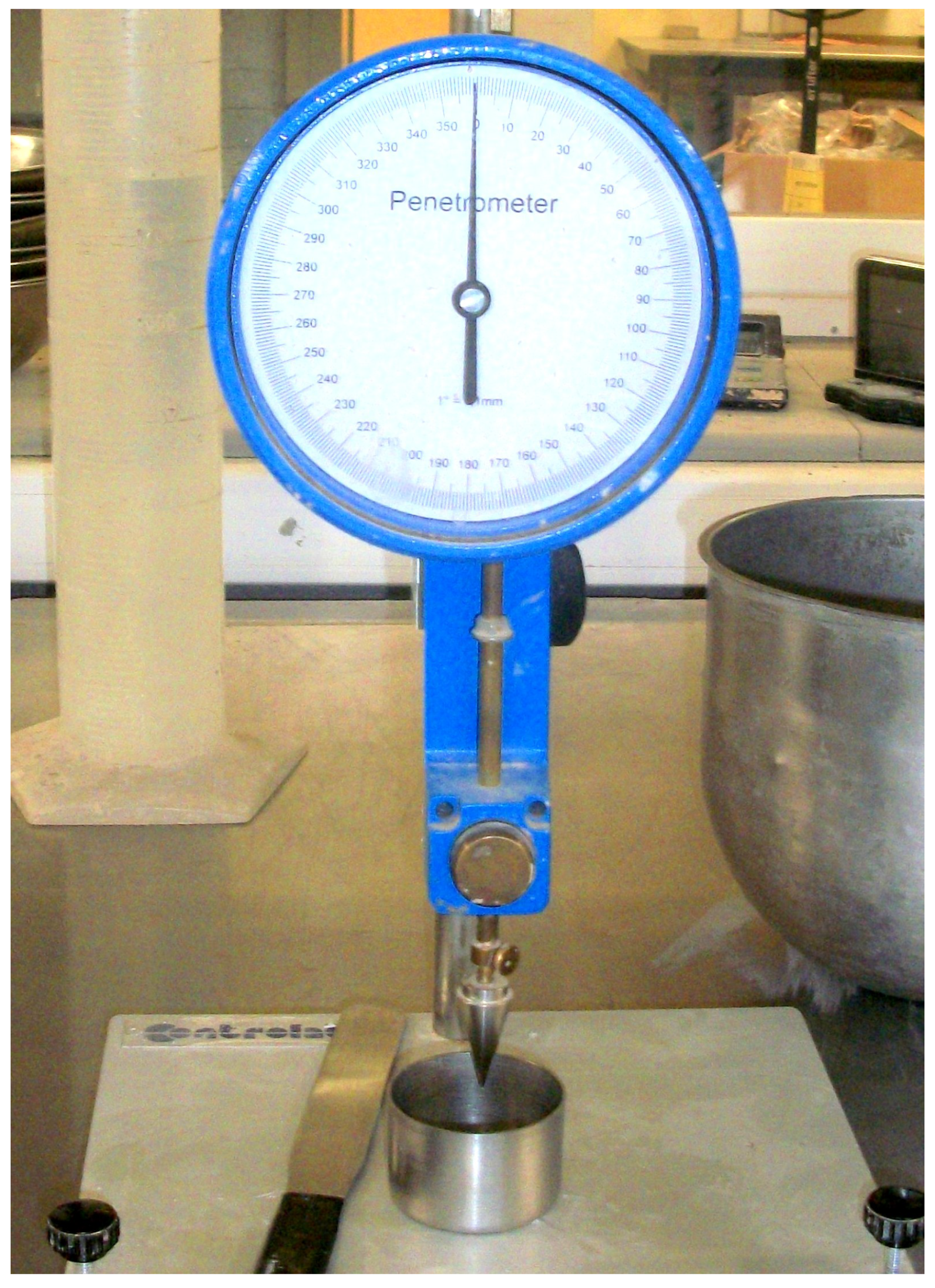
Figure 3.
Sample surface views at different fall cone depths of penetration. Penetration Depth: A = 17.1 mm, B = 14.7 mm, C = 9.7 mm and D = 7.9 mm.
Figure 3.
Sample surface views at different fall cone depths of penetration. Penetration Depth: A = 17.1 mm, B = 14.7 mm, C = 9.7 mm and D = 7.9 mm.
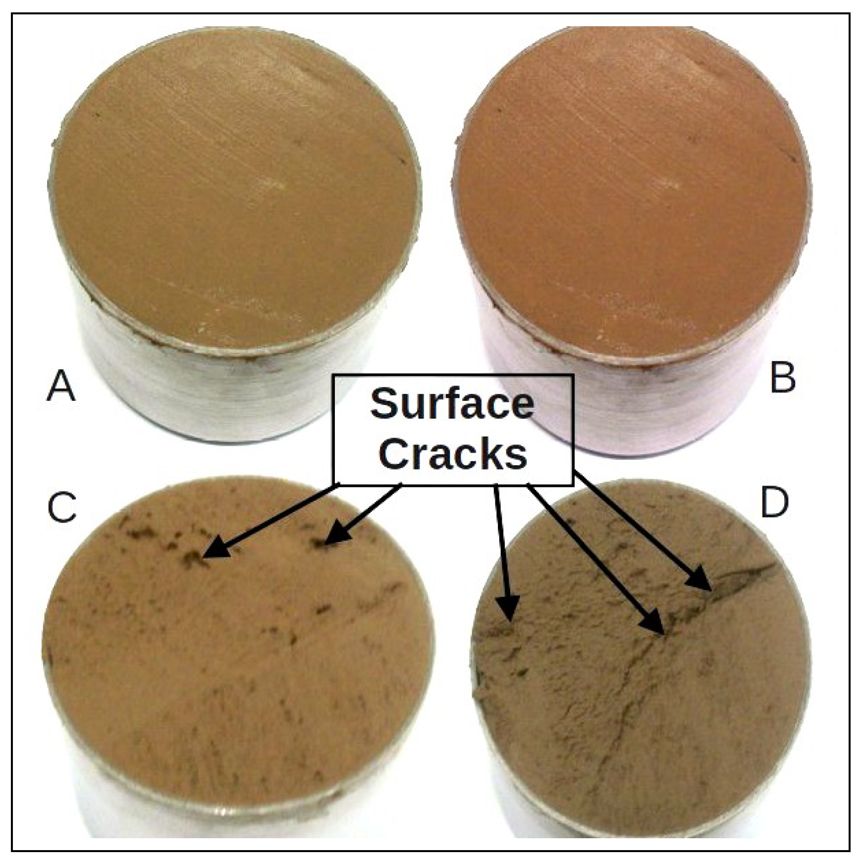
Figure 4.
Linear regression curves of as a function of W/DM.
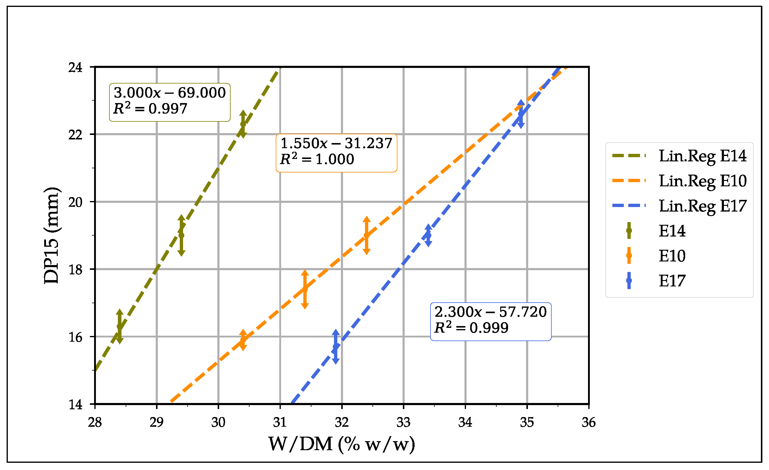
Figure 5.
Fall cone measures’ evolution in time of formulas E4, E7, E14, E17 and E19. Workability from FCPD = 18 mm to FCPD = 10 mm (grey area). (a) Total recorded period; (b) First 120 min.
Figure 5.
Fall cone measures’ evolution in time of formulas E4, E7, E14, E17 and E19. Workability from FCPD = 18 mm to FCPD = 10 mm (grey area). (a) Total recorded period; (b) First 120 min.
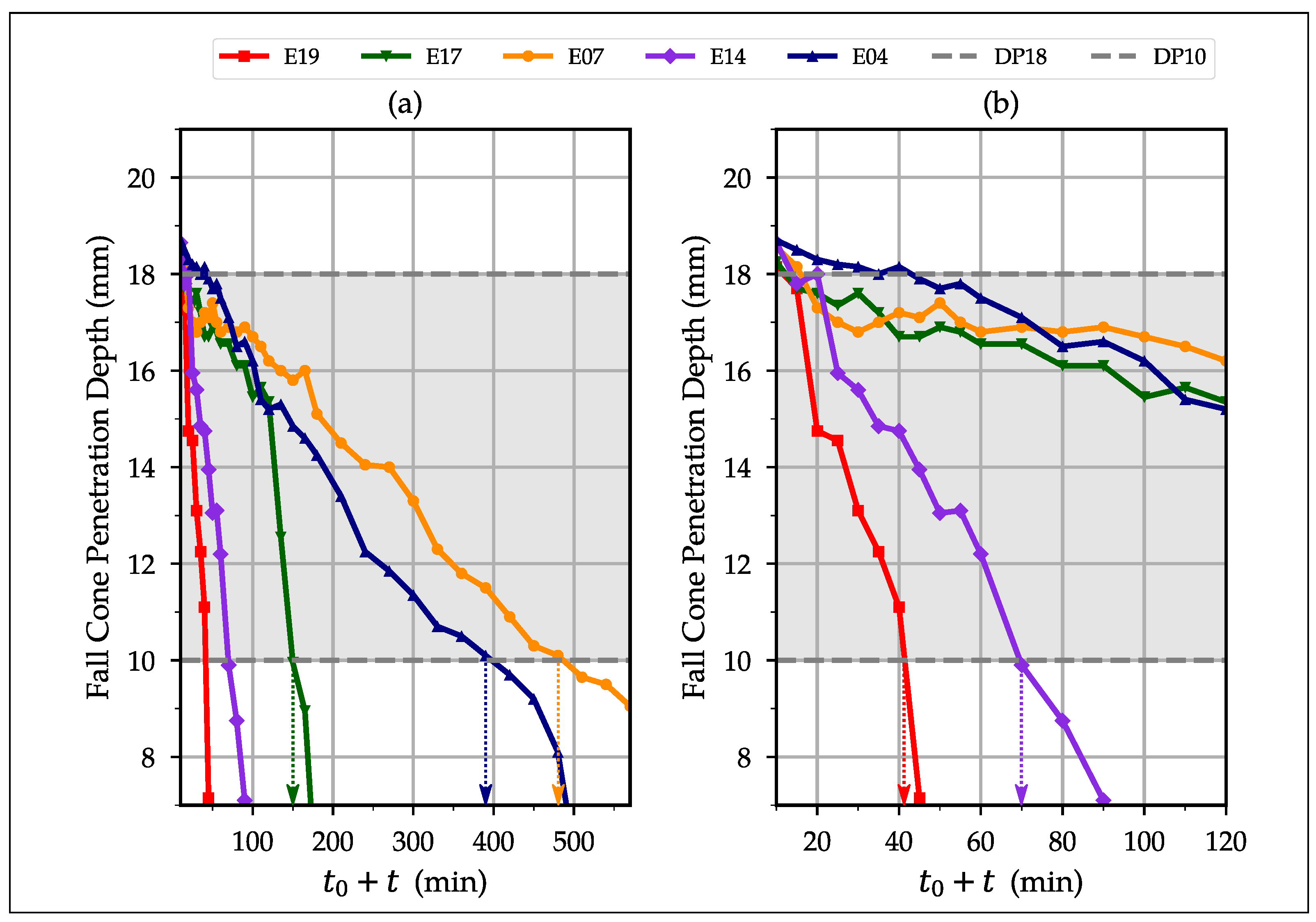
Figure 6.
Evolution of in time (formulas E4, E7, E14, E17 and E19). Workability range (grey area) for from 2.3 kPa (FCPD = 18 mm) to 7.6 kPa (FCPD = 10 mm). (a) Total recorded period; (b) First 120 min.
Figure 6.
Evolution of in time (formulas E4, E7, E14, E17 and E19). Workability range (grey area) for from 2.3 kPa (FCPD = 18 mm) to 7.6 kPa (FCPD = 10 mm). (a) Total recorded period; (b) First 120 min.

Figure 7.
3D printing test: (a) Production line; (b) Test in progress; (c) Printed element at hardened state.
Figure 7.
3D printing test: (a) Production line; (b) Test in progress; (c) Printed element at hardened state.
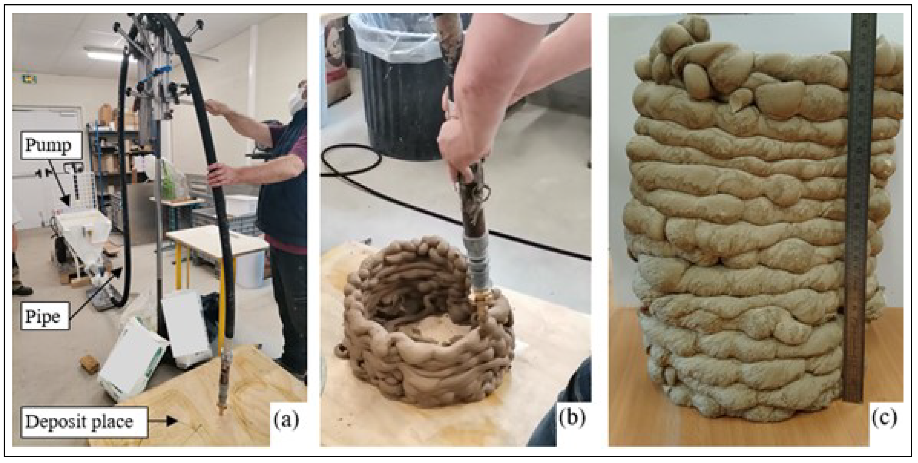
Table 1.
Cement and fly ash main features.
| Mineral Composition (% w/w) | |||
|---|---|---|---|
| Component | OPC | CSAC | FA |
| 20.1 | 8.7 | 43.4 | |
| 5.2 | 18.7 | 7.5 | |
| 2.6 | 7.8 | 21.6 | |
| 64.9 | 43.2 | 11.3 | |
| 1.0 | UD a | 2.0 | |
| 3.7 | 15.3 | 2.8 | |
| eq | 0.67 | 0.20 | 3.34 |
| 0.01 | 0.04 | 0.13 | |
| Physical Properties | |||
| Loss on ignition (% w/w) | 1.4 | 3.4 | 4.1 |
| Specific gravity | 3110 | 2980 | 2570 |
| Blaine specific surface | 4612 | 4520 | 6018 |
a UD = Unavailable Data.
Table 2.
Study levels for each parameters.
| Parameter | Level 1 | Level 2 | Level 3 | Level 4 | Mean Level (2.5) a |
|---|---|---|---|---|---|
| P1: HB in DM (% w/w) | 25.0 | 33.3 | 41.7 | 50.0 | 37.5 |
| P2: CAM added (% w/w) | 0.4 | 0.6 | 0.8 | 1.0 | 0.7 |
| P3: OPC in CM (% w/w) | 0.0 | 33.3 | 66.7 | 100.0 | 50.0 |
| P4: FA in HB (% w/w) | 0.0 | 8.0 | 16.0 | 24.0 | 12.0 |
a Mean Level (2.5) values were calculated to fit with the centre of our experimentation domain (E17).
Table 3.
Mix design.
| Formula | Dry Mixes Composition (g/kg DM) | ||||
|---|---|---|---|---|---|
| CSAC | OPC | FA | QF | CAM | |
| E1 | 250.0 | 0.0 | 0.0 | 750.0 | 4.0 |
| E2 | 153.2 | 76.8 | 20.0 | 750.0 | 6.0 |
| E3 | 70.0 | 140.0 | 40.0 | 750.0 | 8.0 |
| E4 | 0.0 | 190.0 | 60.0 | 750.0 | 10.0 |
| E5 | 186.6 | 93.2 | 53.4 | 666.8 | 4.0 |
| E6 | 253.2 | 0.0 | 80.0 | 666.8 | 6.0 |
| E7 | 0.0 | 333.2 | 0.0 | 666.8 | 8.0 |
| E8 | 102.2 | 204.4 | 26.6 | 666.8 | 10.0 |
| E9 | 105.6 | 211.0 | 100.0 | 583.4 | 4.0 |
| E10 | 0.0 | 350.0 | 66.6 | 583.4 | 6.0 |
| E11 | 383.2 | 0.0 | 33.4 | 583.4 | 8.0 |
| E12 | 277.8 | 138.8 | 0.0 | 583.4 | 10.0 |
| E13 | 0.0 | 460.0 | 40.0 | 500.0 | 4.0 |
| E14 | 166.8 | 333.2 | 0.0 | 500.0 | 6.0 |
| E15 | 253.2 | 126.8 | 120.0 | 500.0 | 8.0 |
| E16 | 420.0 | 0.0 | 80.0 | 500.0 | 10.0 |
| E17 a | 165.0 | 165.0 | 45.0 | 625.0 | 7.0 |
| E18 | 0.0 | 250.0 | 0.0 | 750.0 | 4.0 |
| E19 | 500.0 | 0.0 | 0.0 | 500.0 | 4.0 |
| E20 | 0.0 | 500.0 | 0.0 | 500.0 | 4.0 |
a Formula E17 matches with the centre of the experimentation domain.
Table 4.
Relations between dry mix components and parameters.
| Component Ratio | CAM/DM | QF/DM | FA/DM | OPC/DM | CSAC/DM |
|---|---|---|---|---|---|
| Relation to parameters | P2 | (1 − P1) | P1 × P4 | P1 × P3 × (1 − P4) | P1 × (1 − P3) × (1 − P4) |
Table 5.
Water dosage and bulk density results.
| Formula | E1 | E2 | E3 | E4 | E5 | E6 | E7 | E8 | E9 | E10 | E11 |
| (% w/w) | 33.5 | 34.2 | 35.5 | 35.9 | 33.4 | 34.2 | 32.3 | 33.4 | 33.0 | 31.8 | 32.3 |
| WSC | 2.35 | 2.00 | 1.98 | 1.68 | 2.05 | 2.40 | 2.05 | 2.10 | 2.65 | 1.55 | 2.25 |
| (% w/w) | 32.6 | 33.2 | 34.5 | 34.7 | 32.5 | 33.4 | 31.3 | 32.5 | 32.2 | 30.5 | 31.4 |
| (% w/w) | 34.3 | 35.2 | 36.5 | 37.1 | 34.4 | 35.0 | 33.3 | 34.4 | 33.7 | 33.1 | 33.2 |
| Bulk Density (kg·m) | 1837 | 1827 | 1810 | 1810 | 1830 | 1817 | 1883 | 1857 | 1853 | 1883 | 1863 |
| Formula | E12 | E13 | E14 | E15 | E16 | E17 | E18 | E19 | E20 | E17 | E17 |
| (% w/w) | 32.4 | 29.6 | 29.0 | 32.7 | 32.0 | 32.9 | 33.2 | 29.4 | 28.8 | 32.1 | 33.8 |
| WSC | 2.75 | 2.50 | 3.00 | 2.15 | 2.60 | 2.30 | 1.70 | 2.90 | 2.20 | 2.30 | 2.30 |
| (% w/w) | 31.6 | 28.8 | 28.3 | 31.8 | 31.2 | 32.1 | 32.0 | 28.7 | 27.9 | 32.1 | |
| (% w/w) | 33.1 | 30.4 | 29.7 | 33.7 | 32.8 | 33.8 | 34.4 | 30.1 | 29.7 | 33.8 | |
| Bulk Density (kg·m) | 1880 | 1927 | 1937 | 1870 | 1860 | 1863 | 1847 | 1903 | 1950 | 1867 | 1857 |
E17min and E17Max corresponds to formula E17 mixed with, respectively, the minimal (WDM16) and maximal (WDM20) water amount required to comply with the acceptance criterion.
Table 6.
Printability dosage and bulk density results. limits (min) and initial setting times (min).
Table 6.
Printability dosage and bulk density results. limits (min) and initial setting times (min).
| Formula | E1 | E2 | E3 | E4 | E5 | E6 | E7 | E8 | E9 | E10 | E11 |
| Print Lim (min) | 63 | 94 | 331 | 402 | 52 | 86 | 490 | 311 | 137 | 370 | 70 |
| IST (min) | 140 | 210 | 660 | 1590 | 110 | 200 | 1020 | 530 | 280 | 1460 | 210 |
| IST/Print Lim | 2.00 | 2.10 | 2.06 | 3.79 | 2.20 | 2.35 | 2.13 | 1.66 | 2.07 | 3.74 | 3.00 |
| Formula | E12 | E13 | E14 | E15 | E16 | E17 | E18 | E19 | E20 | E17 | E17 |
| Print Lim (min) | 171 | 272 | 70 | 226 | 135 | 150 | 420 | 42 | 213 | 139 | 181 |
| IST (min) | 290 | 470 | 140 | 380 | 260 | 255 | 1220 | 80 | 420 | 230 | 260 |
| IST/Print Lim | 1.66 | 1.74 | 2.00 | 1.69 | 1.93 | 1.70 | 2.90 | 2.00 | 2.00 | 1.64 | 1.53 |
Table 7.
Summary of the best empirical functions for Print Lim and IST prediction *.
| Print Lim = | IST = | ||||||||
|---|---|---|---|---|---|---|---|---|---|
| Model | a | x | (%) | NRMSD (%) | Model | a | x | (%) | NRMSD (%) |
| P1S060 | 12.07 | −0.87 | 93.5 | 14.9 | I1S060 | 30.42 | −0.79 | 94.8 | 14.9 |
| P1S090 | 15.79 | −0.77 | 98.1 | 15.0 | I1S090 | 40.45 | −0.68 | 94.8 | 27.1 |
| P1S120 | 15.75 | −0.77 | 97.9 | 13.5 | I1S120 | 40.42 | −0.68 | 94.4 | 24.4 |
| P1S150 | 14.95 | −0.80 | 98.5 | 10.1 | I1S150 | 38.46 | −0.70 | 95.4 | 15.9 |
| P1S180 | 14.86 | −0.80 | 98.6 | 9.4 | I1S180 | 38.32 | −0.71 | 95.3 | 16.4 |
* E17 was removed from the regression data set because its workability curve exhibits an unusual profile during the first 120 min.
Table 8.
Parameters Effects Matrix.
| Measured Responses | ||||||||
|---|---|---|---|---|---|---|---|---|
| Effects | Density | WSC | Print Lim | IST | IST/Print Lim | |||
| b0 | 1810.4 | 33.87 | 33.03 | 34.64 | 2.400 | −67.0 | −290.4 | 1.966 |
| b1 | 26.7 | −1.32 | −1.25 | −1.38 | 0.182 | −34.7 | −102.2 | −0.174 |
| b2 | −2.9 | 0.39 | 0.38 | 0.41 | −0.016 | 40.6 | 91.2 | 0.003 |
| b3 | 10.7 | −0.20 | −0.27 | −0.12 | −0.150 | 94.6 | 282.7 | 0.161 |
| b4 | −15.3 | 0.71 | 0.69 | 0.75 | −0.083 | −1.2 | 50.7 | 0.142 |
| Statistical Information | ||||||||
| Mean | 1865 | 32.5 | 31.6 | 33.4 | 2.26 | 205.3 | 497.0 | 2.26 |
| RMSD | 6.66 | 0.38 | 0.31 | 0.31 | 0.25 | 63.60 | 253.30 | 0.59 |
| NRMSD (%) | 0.4 | 1.2 | 1.0 | 0.9 | 11.0 | 31.0 | 51.0 | 26.0 |
Table 9.
Component Effects Matrix.
| Measured Responses | ||||||||
|---|---|---|---|---|---|---|---|---|
| Effects | Density | WSC | Print Lim | IST | IST/Print Lim | |||
| c | 2067.3 | 20.06 | 20.06 | 20.02 | 4.660 | −542.6 | −1933.2 | 0.008 |
| c | 2157.1 | 18.57 | 18.05 | 19.09 | 3.444 | 182.1 | 102.5 | 0.954 |
| c | 1635.1 | 42.15 | 41.08 | 43.57 | 0.968 | −15.7 | 729.1 | 3.953 |
| c | 1753.0 | 37.11 | 35.93 | 38.25 | 1.524 | 166.3 | 621.1 | 3.017 |
| c | −1065.6 | 196.07 | 188.01 | 207.99 | −15.806 | 24,367.2 | 58,653.4 | 10.986 |
| Statistical Information | ||||||||
| Mean | 1865 | 32.5 | 31.6 | 33.4 | 2.26 | 205.3 | 497.0 | 2.26 |
| RMSD | 5.14 | 0.25 | 0.31 | 0.23 | 0.25 | 77.06 | 303.15 | 0.61 |
| NRMSD (%) | 0.3 | 0.8 | 1.0 | 0.7 | 11.0 | 37.5 | 61.0 | 27.0 |
Table 10.
Compressive strengths (MPa) according to curing time, Mean value and standard deviation (SD).
Table 10.
Compressive strengths (MPa) according to curing time, Mean value and standard deviation (SD).
| Formula | 24 h | 28 Days | ||
|---|---|---|---|---|
| Mean Value | SD | Mean Value | SD | |
| E1 | 1.60 | 0.045 | 9.60 | 0.452 |
| E2 | 2.70 | 0.141 | 7.50 | 0.568 |
| E3 | 1.50 | 0.052 | 6.50 | 0.301 |
| E4 | 0.06 | NA | 3.00 | 0.107 |
| E5 | 3.80 | 0.074 | 12.50 | 0.503 |
| E6 | 2.00 | 0.074 | 9.90 | 0.701 |
| E7 | 0.20 | 0.008 | 4.60 | 0.129 |
| E8 | 2.50 | 0.098 | 9.00 | 0.294 |
| E9 | 4.20 | 0.077 | 9.50 | 0.277 |
| E10 | 0.20 | 0.014 | 4.80 | 0.112 |
| E11 | 2.50 | 0.207 | 22.80 | 0.086 |
| E12 | 5.00 | 0.433 | 15.20 | 0.524 |
| E13 | 0.80 | 0.021 | 21.70 | 0.731 |
| E14 | 9.30 | 0.355 | 18.40 | 0.488 |
| E15 | 3.50 | 0.153 | 10.00 | 0.133 |
| E16 | 2.70 | 0.072 | 20.10 | 0.596 |
| E17 | 4.80 | 0.179 | 11.50 | 0.974 |
| E18 | 0.20 | 0.010 | 9.40 | 0.145 |
| E19 | 5.80 | 0.410 | 36.90 | 0.937 |
| E20 | 0.60 | 0.014 | 23.40 | 0.889 |
Table 11.
Measured shrinkage ().
| Formula | Curing Time | |||||
|---|---|---|---|---|---|---|
| 7 Days | 28 Days | 180 Days | ||||
| Mean Value | SD | Mean Value | SD | Mean Value | SD | |
| E1 | −11 | 0 | −11 | 0 | −11 | 0 |
| E2 | −4 | 0.44 | −4 | 0.44 | −5 | 0.44 |
| E3 | −11 | 0.88 | −11 | 1.32 | −11 | 0.88 |
| E4 | −50 | 0.02 | −50 | 0.02 | −51 | 0.02 |
| E5 | −5 | 0.42 | −5 | 0.42 | −5 | 0.02 |
| E6 | −7 | 0.88 | −7 | 0.44 | −7 | 0.88 |
| E7 | −40 | 0.46 | −40 | 0.9 | −41 | 0.9 |
| E8 | −10 | 0.87 | −11 | 0.87 | −11 | 0.43 |
| E9 | −6 | 0 | −6 | 0 | −6 | 0 |
| E10 | −33 | 0.51 | −33 | 0.51 | −34 | 0.96 |
| E11 | −7 | 0.02 | −7 | 0.02 | −7 | 0.02 |
| E12 | −2 | 0 | −3 | 0.44 | −3 | 0 |
| E13 | −20 | 0.87 | −22 | 0.87 | −22 | 0.87 |
| E14 | −3 | 0.44 | −4 | 0.43 | −4 | 0.43 |
| E15 | −3 | 0 | −3 | 0.44 | −3 | 0.44 |
| E16 | −5 | 0.43 | −5 | 0.43 | −6 | 0.43 |
| E17 | −3 | 0.45 | −3 | 0.45 | −4 | 0.01 |
| E18 | −26 | 2.23 | −29 | 1.79 | −30 | 1.79 |
| E19 | −6 | 0 | −6 | 0 | −7 | 0 |
| E20 | −22 | 0.41 | −23 | 0.85 | −25 | 0.41 |
Publisher’s Note: MDPI stays neutral with regard to jurisdictional claims in published maps and institutional affiliations. |
© 2022 by the authors. Licensee MDPI, Basel, Switzerland. This article is an open access article distributed under the terms and conditions of the Creative Commons Attribution (CC BY) license (https://creativecommons.org/licenses/by/4.0/).
Share and Cite
MDPI and ACS Style
D’Haese, R.; Carpentier, O.; Dubois, V.; Chafei, S.; Wirquin, E. 3D-Printable Materials Made with Industrial By-Products: Formulation, Fresh and Hardened Properties. Sustainability 2022, 14, 14236. https://doi.org/10.3390/su142114236
AMA Style
D’Haese R, Carpentier O, Dubois V, Chafei S, Wirquin E. 3D-Printable Materials Made with Industrial By-Products: Formulation, Fresh and Hardened Properties. Sustainability. 2022; 14(21):14236. https://doi.org/10.3390/su142114236
Chicago/Turabian StyleD’Haese, Romain, Olivier Carpentier, Vincent Dubois, Sawsen Chafei, and Eric Wirquin. 2022. "3D-Printable Materials Made with Industrial By-Products: Formulation, Fresh and Hardened Properties" Sustainability 14, no. 21: 14236. https://doi.org/10.3390/su142114236
Note that from the first issue of 2016, this journal uses article numbers instead of page numbers. See further details here.