
An Experimental Study on Performance Evaluation of Shading Matrix to Select Optimal Parking Space for Solar-Powered Electric Vehicles


1
Energy Resources Institute, Pukyong National University, Busan 48513, Korea
2
Department of Energy Resources Engineering, Pukyong National University, Busan 48513, Korea
*
Author to whom correspondence should be addressed.
Sustainability 2022, 14(22), 14922; https://doi.org/10.3390/su142214922
Submission received: 16 October 2022
/
Revised: 9 November 2022
/
Accepted: 9 November 2022
/
Published: 11 November 2022
(This article belongs to the Section Sustainable Transportation)
Abstract
:This study evaluated the applicability of a shading matrix generated using hemispherical fisheye images to select the optimal parking space to maximize the photovoltaic (PV) power generation of solar electric vehicles. The study aims to identify the maximum power point (MPP) of a PV module in a parking space using current–voltage measuring equipment to determine whether the shading matrix reflects any shadow phenomenon. The experiment was conducted on a parking lot at Daeyeon Campus. The fisheye images were taken in seven parking spaces. The shading matrices were generated by tracking the position of the sun over 12 months and 24 h periods. A 50 W PV module was installed on the roof of the vehicle and the MPP was measured in five experiments (9 a.m., 11 a.m., 13 p.m., 15 p.m., and 17 p.m.) in seven parking spaces. In parking spaces with a shading factor of 0, the PV modules were not shaded at all during the experiment, and the average MPPs were 34, 43, 37, and 21 W at 9 a.m., 11 a.m., 13 p.m., and 15 p.m., respectively. The shading matrix calculated using the fisheye images accurately reflected the shadow phenomenon that decreases PV power generation.
1. Introduction
At the 21st Conference of Parties (COP21) in 2015, the Paris Agreement was adopted to reduce worldwide greenhouse gas (GHG) emissions [1]. In this agreement, developed and developing countries agreed to establish (by 2030) nationally determined contributions (NDC) and evaluate the feasibility of achieving this goal through global stocktaking every five years from 2035 [2]. In 2018, the “Global warming of 1.5 °C special report” [3] published by the Intergovernmental Panel on Climate Change (IPCC) initially proposed to reach global net-zero carbon emissions by 2050. Accordingly, governments and international organizations around the world are establishing national energy policies and carbon reduction plans for each sector to realize net-zero by 2050. The “Net-Zero Emission by 2050 Scenario (NZE)” [4] was published by the International Energy Agency (IEA) and presented a roadmap for energy policy until 2050 by sector (Electricity, Industry, Transport, and Buildings). The “Mitigation of Climate Change” [5] of the working group III contribution to the sixth assessment report of the IPCC, identifies and evaluates the carbon emission pathways for each system in the various sectors and identifies specific carbon emission reduction methods.
In the road transport sector, the electrification of vehicles plays a major role in net-zero by 2050 [6]. The IEA predicts that the electrification of vehicles would cause CO2 emissions to be reduced by 90% in 2050, compared with approximately 3.2 Gt CO2 in 2020 [7]. Recently, governments around the world have accelerated the transition to electric vehicles (EVs) by tightening fuel efficiency regulations for internal combustion engine vehicles and expanding investment in electric vehicle infrastructure. In the United States, the National Highway Traffic Safety Administration (NHTSA) has regulated the fuel efficiency of passenger cars and light trucks to 49 mpg in 2026 [8]. The United States federal government has invested USD 5 billion to expand the number of public chargers to 500,000 by 2030 [9]. The EU has regulated the CO2 emissions of passenger cars and light trucks to 95 g CO2/km and 147 g CO2/km, respectively, by 2024 [10]. In addition, the EU will expand public charging points to 1 million and 3 million in 2025 and 2030, respectively [11]. Major automakers are rushing to announce electrification plans, accelerating the transition to a fully electric future [12]. Mercedes-Benz and Volvo announced that they will launch only full electric car models by 2025 and 2030, respectively [13,14]. Volkswagen has predicted almost 100% EV sales by 2040 [15].
Automakers and start-ups have launched solar-powered electric vehicles (SPEVs) equipped with solar modules on the vehicle exterior. Solar modules are the assembly of connected solar cells. Solar cells can be classified into silicon-based solar cells, perovskite solar cells, dye-sensitized solar cells, polymer solar cells, etc. depending on the materials [16,17,18,19]. SPEVs generate electricity from solar energy and self-charge their batteries while driving and parked [20]. SPEVs began to be rapidly introduced into the automobile market for reasons of the long and frequent EV battery charging requirements, improved efficiency of solar cells, global solar cell price decline, global EV market growth, etc. The charged electricity increases the driving range and operates the air conditioning system [21]. The solar module can be attached to the EV exterior, such as the roof, hood, side doors, and rear hatch doors. The SPEV models include Lightyear One (Lightyear) [22], Solar Roof (Hyundai Motor Group) [23], Luna (Aptera Motors) [24], Sion (Sono Motors) [25], Vision EQXX (Mercedes-Benz Group) [26], and bZ4X (Toyota Motor Corporation) [27]. In 2027, the average annual growth rate of the SPEV market will reach approximately 20%, with a market size of approximately USD 689 billion [28].
Various SPEV models have recently been released in the EV market. The software technology for effectively operating solar electric vehicles is actively being developed. SPEV operation technologies are broadly classified into two categories. The first is navigation technology that analyzes the optimal driving route to maximize photovoltaic (PV) power generation and minimize energy consumption while driving. Recent research includes speed planning on road segments [29], solar PV energy mapping [30], and route planning considering solar insolation, shadow effect, road slope, travel time, traffic flow, energy consumption, and solar power generation [31,32,33,34]. The second category is technology to analyze optimal parking lots and parking spaces to maximize PV power generation when parked. Choi et al. [35] selected the optimal parking lot for SPEVs on a university campus by analyzing the shadow effect from fisheye imagery.
A factor that greatly influences PV generation during parking is the shadows caused by shading obstructions in urban areas, such as buildings, trees, and electric wires. If the PV modules of the SPEVs are partially or fully shaded, PV power generation is significantly reduced. Therefore, to maximize the PV power generation of SPEVs during parking, it is necessary to select parking spaces with the least shadow effects. The shadow shape can vary every hour, depending on the position of the sun. In addition, the shape of the shadow may vary with season, owing to the seasonal variations in sun altitude. Therefore, it is necessary to analyze the effects of shadows that change with time and season in each parking space. The representative shadow analysis method uses fisheye images. In this method, fisheye images are captured using a digital camera with an ultra-wide fisheye lens and shading obstructions in the fisheye image are identified using image processing [36]. While tracking the position of the sun with the season and time, a shading factor between 0 and 1 (0: open sky, 1: fully shaded) is calculated based on the presence or absence of shading obstructions [37]. The data formed a shading matrix with rows and columns at 12 months and 24 h. The matrix enables an accurate shadow analysis in urban areas because it can accurately and quickly capture the sophisticated shapes of shading obstructions and seasonal changes using fisheye imaging.
Selecting a parking space for SPEVs using the shading matrix provides the optimal parking space by determining the parking space with the lowest mean shading factor for a day, month, quarter, and year. In addition, it is possible to predict the approximate PV power generated by the SPEV. To do this, it is necessary to evaluate whether the hourly and seasonal shading factors of the shading matrix reflect the actual shadow phenomenon and corresponding to decreases in the PV power generation. However, no previous research has analyzed whether the shading matrix formed using fisheye images can reflect the actual shadow phenomenon and decrease in PV power generation. In addition, no research has evaluated the applicability of the shading matrix using fisheye images to select the optimal parking space for SPEVs.
The purpose of this study is to evaluate the applicability of the shading matrix using hemispherical images to select the optimal parking space for SPEVs. The fisheye images were used to create a shading matrix for seven different parking spaces in the parking lot of the Daeyeon Campus of Pukyong National University. At 9 a.m., 11 a.m., 13 p.m., 15 p.m., and 17 p.m., the maximum power point (MPP) was measured in seven different parking spaces using PV modules and I–V measuring equipment. By comparing the shading matrix and MPP results, the applicability of the shading matrix as a tool for selecting optimal parking spaces was evaluated.
This paper is organized as follows. Section 2 describes the study area in which the experiment was performed. Section 3 introduces the experimental equipment and settings. Section 4 presents the results of the MPP measurements in five experiments (9 a.m., 11 a.m., 13 p.m., 15 p.m., and 17 p.m.) and compares the shading matrix and MPP results, followed by the discussion and conclusions in Section 5 and Section 6.
2. Study Area
The Daeyeon Campus of Pukyong University (35°08′02″ N, 129°06′10″ E) is located in Nam-gu, Busan, Republic of Korea and was selected for this research project. The location consists of relatively flat terrain with an elevation of approximately 3–10 m above the sea level. In this study, one campus parking lot was selected for the experiment. Figure 1 provides a birds-eye view of the parking lot. The size of each parking space is approximately 2.5 m wide and 5 m long, with an area of about 12.5 m2. To the east of the parking lot was the six-story Narae building and the four-story Design building. The west side of the parking lot was lined with trees that were approximately 13 m tall. Most of the parking space was shaded by buildings to the east and trees to the west. Therefore, selecting the optimal parking space for SPEVs in the parking lot requires consideration of the decrease in PV power generation owing to shadows during the year, quarter, and day.
3. Experimental Methods
3.1. Experimental Equipment
Three types of equipment were used in this research. The first is the Solmetric SunEye 210 [38]. Figure 2a provides a photograph using SunEye 210. The SunEye 210 captures fisheye images, analyzes shadows caused by shading obstructions, and calculates shading factors. The ultrawide-angle fisheye lens mounted on the instrument can capture all objects within 180° including vertical, horizontal, and diagonal angles in one image. The equipment was placed in the south-facing direction (180° azimuth) to track the path of the sun. The open sky and any shading obstructions (including buildings and trees) in the fisheye image were automatically classified through image processing. The coordinates of the sun’s position were calculated with the fisheye image using the survey point latitude, date of the year, and time of the day. If shading obstructs the position of the sun in the fisheye image, the shading factor is calculated as 1. If no shading obstructs the position of the sun, the shading factor is calculated as 0. Figure 2b provides an example of a fisheye image. The yellow area in the image is a sun-path diagram showing the position of the sun according to the time of day. The green area represents the shading obstructions on the sun-path diagram. For example, the shading factor at 9 a.m. in September was 1. In contrast, the shading factor at 13 p.m. in September was 0. The shading factor is calculated by repeatedly tracking the position of the sun for 24 h over 365 days a year at 15 min intervals. The shading factors were averaged in units of 1 h. A shading matrix was generated by transforming all the shading factors into a month-by-hour matrix. This equipment can calculate the shading matrix in real time using a fisheye image.
The second device used in this experiment was a PV analyzer from Solmetric [39] (Figure 3a). A PV analyzer measures the current–voltage characteristics of the PV modules and identifies the MPP. Table 1 lists the PV analyzer specifications. The equipment was connected to the PV module using a MC-4 connector, which measures any current ranging from 0–20 A dc and a voltage range of 20–600 V dc while increasing the resistance of the PV module from 0 to ∞. Figure 3b provides an example of the I–V curve and P–V curves. When the resistance is 0 (i.e., short circuit), the current is expressed as Isc and when the resistance is ∞ (i.e., open circuit), the voltage is expressed as Voc. The point when the voltage and current reach a maximum is expressed as the MPP. The voltage and current at MPP is expressed as Vmp and Imp, respectively. The device was connected to a portable PC within a range of 10 m using a wireless USB adapter. The third device used in this experiment was a 50 W PV module (Figure 3c). Table 2 lists the specifications of the PV modules. The PV module consisted of 18 solar cells and was manufactured as a flexible-type module. Under ideal conditions, the Vmp of the PV module is approximately 18 V and the Imp is approximately 2.78 A.
3.2. Experimental Settings
Seven parking spaces in the parking lot were randomly selected as survey points. Figure 4a highlights the positions of the seven survey points. All survey points were shaded by surrounding buildings and trees as the position of the sun changed throughout the day. The survey points 1, 4, and 6 were close to the trees in the west, which causes shadows in the early afternoon. Conversely, survey points 2 and 3 were shaded throughout the morning by the building on the east. Survey points 5 and 7 were relatively less affected by shadows from buildings and trees during the morning and afternoon hours. In this study, 9 a.m., 11 a.m., 13 p.m., 15 p.m., and 17 p.m. were the experiment times when the data were collected to analyze changes in the MPP of the PV module according to the shadow effects that can vary throughout the day. The experiment times were selected to coincide with the car parking time of the working day. An interval of two hours was set between the experiment times to avoid inaccuracy due to experiment confusion and haste. It was assumed that solar insolation was constant during the experiment and the MPP of the PV module was only impacted by the shadows. Table 3 lists the solar insolation results on 18 June 2022. June was chosen because it had the longest daylight over a 12-month period in the study area and was able to measure the MPP for many experiment times. The fisheye images were captured at seven survey points using SunEye 210 equipment and seven shading matrices were formulated. In addition, the shading factors were calculated at 9 a.m., 11 a.m., 13 p.m., 15 p.m., and 17 p.m. in June. Figure 4b,c demonstrate a vehicle equipped with a PV module, PV analyzer, and laptop PC. The PV module was placed on the roof of the vehicle. The PV analyzer was controlled using a laptop computer. For each experiment, the vehicle was parked at one of the seven survey points. The MPP measurement of the PV module was repeated five times for each survey point and the results of the five measurements were averaged.
4. Results
The fisheye images were captured at seven survey points and shading obstructions were analyzed by image processing. Figure 5 shows fisheye images from the seven survey points. The sun-path diagrams revealed survey points 1, 2, and 3 had buildings as shading obstructions in the morning in most seasons and trees were classified as shading obstructions in the afternoon (Figure 5a–c). The trees were classified as shading obstructions after 12 p.m. in all seasons at survey points 4 and 6. The remaining survey points (5 and 7) had shading obstruction by the buildings and trees in the early morning and late afternoon in all seasons.
The analysis of the fisheye images revealed the shading factors with time over one year to form a shading matrix. Figure 6 shows the shading matrix of the seven survey points. The shading factor was 1 if the season and time corresponded with the buildings and trees shading the survey point on the sun-path diagram and 0 if there was no shading. The shading factor was calculated as a value between 0 and 1 with shading obstruction within a 1 h timeframe. In the shading matrix, the solid dark line indicates the shading factor corresponding to the experiment time. Table 4 lists the shading factors recorded at each time at each survey point. For example, at survey point 3 at 9 a.m. in June, the shading factor was calculated as 1 because a shadow was generated by the building to the east.
The shading factor of survey points 1, 4, and 6 were calculated as 1 because tree shadows occurred over these parking spaces in the afternoon. Conversely, at survey points 2, 5, and 7, there were no shading obstructions from 9 a.m. to 15 p.m.; therefore, the shading factor was calculated as 0. At 17 p.m. in June, all survey points had a shading factor of 1 because the sun was obscured by trees. Figure 7 provides the PV module results captured at 11 a.m. and 13 p.m. at survey point 4. The shading factor at 11 a.m. was calculated as 0 (no shadows existed at this time). At 13 p.m., the shading factor was 0.8 because the PV module was partially obscured by the shadow of a tree.
At 9 a.m., 11 a.m., 13 p.m., 15 p.m., and 17 p.m., the MPP of the PV module was measured at all seven survey points. The MPP and shading factors were compared. Figure 8 shows the experimental results at 9 a.m. and the inner and outer circles represent the shading factor distribution with the average MPP, respectively. When the two circles are the same color, an inverse relationship between the shading factor and the MPP has been established. An average MPP of approximately 34 W was observed at survey points 1, 2, 4, 5, 6, and 7. In contrast, survey point 3 had a relatively low average MPP of approximately 10 W. The PV module at survey point 3 was fully shaded by the building on the east side. The average Vmp and Imp of survey points 1, 2, 4, 5, 6, and 7 were approximately 16.43 V and 2.04 A. Conversely, the average Vmp and Imp of survey point 3 was 15.86 V and 0.62 A, respectively. At survey point 3 the Imp was less than 70% of the other points. The results revealed that when the factor is 1, a shadow occurs over the PV module and the MPP significantly decreases.
Figure 9 provide the MPP results at 11 a.m. at all seven survey points. The average MPP was approximately 43 W. The insolation increased from 9 a.m. and the average MPP at 11 a.m. had increased by approximately 1.3 times the levels of 9 a.m. The average Vmp and average Imp at all survey points were 15.6 V and 2.63 A, respectively. The MPP was high when the shading factor at each survey point was 0.
Figure 10 shows the MPP, I–V curve, and P–V curve measured at all seven survey points at 13 p.m. The shading factors of survey points 1, 2, 3, 5, and 7 were 0 and the average MPPs were 40, 39, 35, 35, and 35 W, respectively. Conversely, the shading factors of the survey points 4 and 6 were 0.85 and 1, respectively, and the average MPP was 3 W and 4 W, respectively. At survey points 4 and 6, the MPP was significantly low due to shadows on the PV modules caused by trees. The average Vmp and average Imp were 15.51 V and 2.38 A at survey points 1, 2, 3, 5, and 7, and only 13.86 V and 0.27 A at survey points 4 and 6. The Imp was lower (by approximately 89%) at survey points 4 and 6 because of the shadows on the PV module. In addition, the I–V and P–V curves of survey points 4 and 6 were not formed because the voltage and current are not measured when the resistance value is high. The results of the experiment at 13 p.m. identified that the MPP significantly decreased because of shadows when the shading factor was close to 1.
Figure 11 shows the MPP, I–V, and P–V curves measured at all seven survey points at 15 p.m. At 15 p.m., the sun was behind the trees to the west, so shadows occurred on the PV modules at survey points 1, 4, and 6. Similarly, the shading factor at survey points 1, 4, and 6 were 1. Therefore, the average MPP of survey points 1, 4, and 6 were 3 W, 2 W, and 6 W, respectively. However, there was no shadow on the PV modules at survey points 2, 3, 5, and 7, and all of their shading factors were 0. Accordingly, the average MPP of these survey sites was approximately 21 W. The average MPP was low due to the limited insolation when compared to the results at 13 p.m. The average Vmp and Imp were approximately 14.03 V and 0.27 A at survey points 1, 4, and 6, and approximately 17.11 V and 1.20 A at the shaded survey points (2, 3, 5, and 7). I–V and P–V curves were not formed at survey points 1, 4, and 6 because the voltage and current was not measured because the resistance was higher than the critical limit.
Figure 12 provides the measured MPP at all seven survey points at 17 p.m. At 17 p.m., the sun was completely obscured by the trees to the west, so no sunlight was present at any of the survey points. Accordingly, the average Vmp and Imp at all survey points were 10.75 V and 0.21 A, respectively. The average MPP was 2 W. The shading factor was calculated to be 1. In addition, it was not possible to measure the voltage and current resistance value at any of the seven survey points.
Figure 13 shows the average MPP measured at each survey point after classifying the time into the shading factor of 0 or above 0. When the shading factor was 0, no shadows were generated on the PV module at any of the survey points. The average MPP when the shading factor was 0 was significantly higher at each time than when the shading factor was higher than 0. In addition, as the level of insolation increases, the average MPP of the irradiation point with a shading factor of 0 also tended to increase. However, when the shading factor was 0 or higher, the PV module was partially or fully shaded by trees and/or buildings. This situation resulted in a low average MPP of approximately 4 W. The results confirmed that the shading matrix using fisheye imaging reflected the shadows on the PV module. In addition, the MPP of the PV module lowered when the shading factor of the shading matrix was above 0. Therefore, the shading matrix using fisheye imaging could be used to select the optimal parking space for SPEVs.
5. Discussion
5.1. Additional Findings from Experiment Results
Any increase in the shading factor did not tend to correspond proportionally with a decrease in the MPP. For example, at survey point 3 at 9 a.m. and 17 p.m., the shading factors were both 1 and the average MPP was 10 W and 5 W, respectively. Similarly, the average MPP of survey points 4 (shading factor: 0.88) and 6 (shading factor: 1) at 13 p.m. were 3 W and 4 W, respectively. The MPP value was determined by both the shape of the shadow and by various factors such as weather conditions, insolation, type of shading obstructions, and PV module issues.
Survey point 3 at 9 a.m. (point 3 in Figure 8) and survey point 6 at 13 p.m. (Point 6 in Figure 10) were quantitatively compared. At 9 a.m., survey point 3 had an average MPP of 10 W because the PV module was fully shaded by a building. At survey point 6 at 13 p.m., the PV module was partially shaded by trees and the average MPP was approximately 4 W. Although the PV module was completely covered by the building at survey point 3, the average MPP was calculated to be higher than at survey point 6 (at 13 p.m.) because a constant low current flowed without any bottleneck. On the other hand, at survey point 6 at 13 p.m., the voltage and current were not able to be measured because a bottleneck occurred due to the partial shadows.
5.2. Selecting an Optimal Parking Space for SPEVs
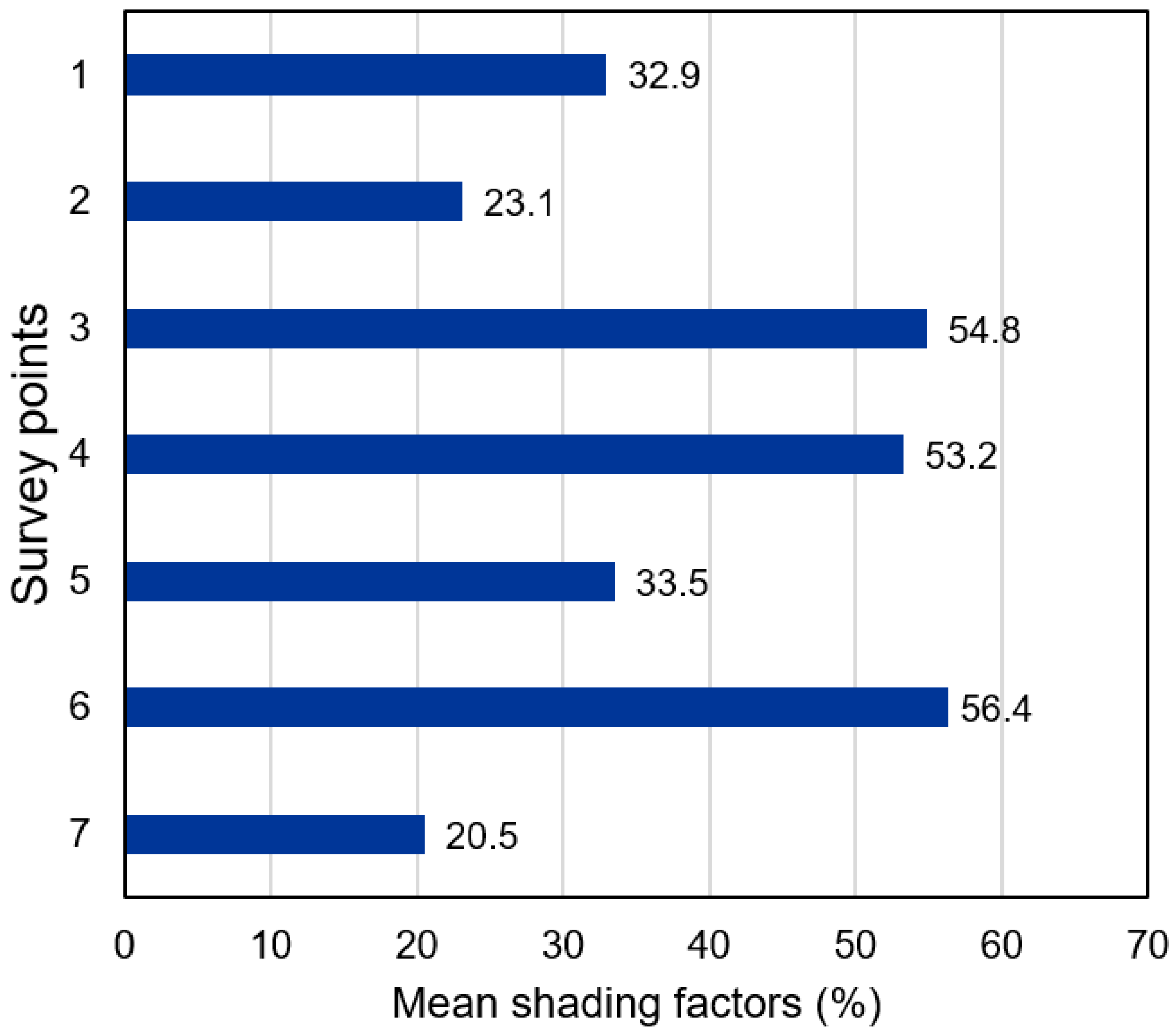
Of the seven parking spaces, the area with the least shadow effect was able to be determined by the shading matrix using fisheye imagery. The mean shading factor for June was calculated using the shading matrix of the seven parking spaces presented in Figure 6. Equation (1) calculated the mean shading factor for June. It is expressed as a percentage of the mean of the shading factors over 13 h, between sunrise (6 a.m.) and sunset (19 p.m.). This equation assumes the sunrise and sunset times of June in the study area (latitude: 129°06’10″ E). The MSFJune is the mean shading factor of June (%) and SF(June, 6AM) is the shading factor at 6 a.m. in June. Figure 14 provides the calculated mean shading factor (%) results for June in the seven parking spaces. A lower mean shading factor corresponds to a lower rate of shadows occurring in the parking space during the potential daily sunshine duration. The mean shading factor was as low as 20.5% (at survey point 7) and 23.1% (at survey point 2). On the other hand, at survey points 3, 4, and 6, the mean shading factors were 54.8%, 53.2%, and 56.4%, respectively. It can be predicted that the accumulated PV power generation in June by the SPEV is the highest at survey point 7. It can also be predicted that the accumulated PV power generation in June by the SPEV is the lowest at survey point 6. The results indicate that the shading matrix formed using fisheye imaging is a useful tool for selecting the optimal parking space for SPEVs.
5.3. Advantages and Disadvantages of Shading Matrix Generation Using the Hemispherical Image
This method includes some advantages to generate shading matrices using hemispherical images. This approach improves the accuracy of shading analysis by taking photographs of the actual shape of buildings and trees. To generate the shading matrix, it is not necessary to build 3D building and tree models using computer-aided design tools. It is possible to produce shading matrices with only the low cost of a digital camera. Therefore, it is less expensive to use this approach for large-scale applications. In addition, it would be possible to easily and sensitively respond to temporal and spatial variation of shading obstructions. Even if the shape of the tree changes according to the season or the buildings are expended or moved, it can be solved by taking the hemispherical images again at the survey points. These advantages can support the selection of the optimal parking space of SPEVs.
Nevertheless, this approach has several disadvantages. It is impossible to take hemispherical images in areas inaccessible to people. Additionally, it is time-consuming to investigate the shading matrix for large and dense points. The field of view of the most commercialized fisheye camera lens is less than 180 degrees due to the low precision. Therefore, it is difficult to capture the shading obstructions within the vertical angle range of 0 to 10 degrees. These shortcomings can be overcome to use hemispherical images in conjunction with unmanned aerial vehicle (UAVs) and 3D model approaches.
6. Conclusions
This study evaluated the applicability of a shading matrix using fisheye images to select the optimal parking space to maximize the PV power generation by SPEVs. The study evaluated whether the shading matrix reflects the decreases in PV power generation by shadows in a parking space. The parking lot of the Daeyeon Campus of Pukyong National University was selected as the experimental site, and seven parking spaces were selected as survey points. The fisheye images were taken at all seven survey points and shading matrices were formed over 12 months for 0 and 24 h. The MPP of the 50 W PV module installed on the vehicle roof was measured at 9 a.m., 11 a.m., 13 p.m., 15 p.m., and 17 p.m. at each survey point. When the shading factor was 0, no shadows were on the PV module and the average MPP reached 34, 43, 37, and 21 W at 9 a.m., 11 a.m., 13 p.m., and 15 p.m., respectively. Conversely, when the shading factor was above 0, the PV module was partially or fully shaded by trees and/or buildings and the average MPP was less than 10 W. The shading matrix created using fisheye images could accurately reflect the shadows caused by trees and buildings and identified the resulting decreases in PV power generation.
It was possible to calculate the mean shading factor (%) for June using the shading matrix at the seven survey points and to analyze the optimal parking space for SPEVs. The mean shading factor was the lowest at 20.5% at survey point 7 and the highest was 56.4% at survey point 6. On average, parking space 7 received the least shadow effect during June and the analyses predicted the accumulated PV power generation by an SPEV would be the highest if parked in this space. Parking space 7 is the optimal parking space for an SPEV. The shading factor generated using a fisheye image is a useful tool for selecting the optimal parking space for solar electric vehicles.
There are a few limitations to measuring the MPP using the PV module and I–V measuring equipment. First are the additional shading effects on the PV system. The dust and abrasion may cause additional shading effects. Therefore, these factors should be considered to measure the MPP of the PV module. Second is diffuse solar radiation. In this study, as presented in Table 3, it was assumed that solar insolation was constant during the experiment. However, some cloud cover will likely impact the level of shading. In the future, it would be possible to consider diffuse solar radiation by providing it as a factor of the MPP calculation. The final limitations are the lack of MPP output comparisons. It is recommended to compare the MPP outputs using various MPP measurement techniques and equipment.
The shading matrix formed using fisheye imagery can be used in SPEV operating software for navigating and selecting optimal parking sites. By calculating the mean shading factor over days, weeks, months, seasons, and a year, it is possible to select an optimal parking space which maximizes the PV power generation by SPEVs. Additionally, it is possible to analyze the optimal driving route of SPEVs by calculating the minimum cumulative shading factor for each driving route. In the future, it would be possible to analyze the optimal driving routes and parking spaces using shading matrices derived from fisheye images for efficient SPEV operations.
Author Contributions
Conceptualization: J.B. and Y.C.; Data curation: J.B. and Y.C.; Formal analysis: J.B. and Y.C.; Funding acquisition: J.B.; Investigation: J.B.; Methodology: J.B. and Y.C.; Project administration: Y.C.; Resources: Y.C.; Software: Y.C.; Supervision: Y.C.; Validation: J.B.; Visualization: J.B.; Roles/Writing—original draft: J.B.; Writing—review and editing: Y.C. All authors have read and agreed to the published version of the manuscript.
Funding
This work was supported by the National Research Foundation of Korea (NRF) grant funded by the Korea government (MSIT) (No. 2022R1C1C2011947).
Informed Consent Statement
Not applicable.
Conflicts of Interest
The authors declare no conflict of interest.
References
- United Nations. The Paris Agreement. Available online: https://unfccc.int/process-and-meetings/the-paris-agreement/the-paris-agreement (accessed on 7 November 2022).
- United Nations. Adoption of the Paris Agreement. Available online: https://unfccc.int/files/essential_background/convention/application/pdf/english_paris_agreement.pdf (accessed on 7 November 2022).
- Intergovernmental Panel on Climate Change (IPCC). Global Warming of 1.5 °C Special Report. Available online: https://www.ipcc.ch/sr15 (accessed on 7 November 2022).
- International Energy Agency (IEA). Net Zero Emissions by 2050 Scenario (NZE). Available online: https://www.iea.org/reports/world-energy-model/net-zero-emissions-by-2050-scenario-nze (accessed on 7 November 2022).
- Intergovernmental Panel on Climate Change (IPCC). Climate Change 2022 Mitigation of Climate Change. Available online: https://report.ipcc.ch/ar6wg3/pdf/IPCC_AR6_WGIII_FinalDraft_FullReport.pdf (accessed on 7 November 2022).
- World Economic Forum (WEF). Circular Economy Is Key to Accelerating Net-Zero Transportation. Here’s Now. Available online: https://www.weforum.org/agenda/2022/05/circular-economy-net-zero-transportation (accessed on 7 November 2022).
- International Energy Agency (IEA). Net Zero by 2050 A Roadmap for the Global Energy Sector. Available online: https://iea.blob.core.windows.net/assets/deebef5d-0c34-4539-9d0c-10b13d840027/NetZeroby2050-ARoadmapfortheGlobalEnergySector_CORR.pdf (accessed on 7 November 2022).
- National Highway Traffic Safety Administration. Corporate Average Fuel Economy. Available online: https://www.nhtsa.gov/laws-regulations/corporate-average-fuel-economy (accessed on 7 November 2022).
- The White House. FACT SHEET: The Biden-Harris Electric Vehicle Charging Action Plan. Available online: https://www.whitehouse.gov/briefing-room/statements-releases/2021/12/13/fact-sheet-the-biden-harris-electric-vehicle-charging-action-plan (accessed on 7 November 2022).
- European Commission. CO₂ Emission Performance Standards for Cars and Vans. Available online: https://ec.europa.eu/clima/eu-action/transport-emissions/road-transport-reducing-co2-emissions-vehicles/co2-emission-performance-standards-cars-and-vans_en (accessed on 7 November 2022).
- European Commission. Sustainable and Smart Mobility Strategy—Putting European Transport on Track for The Future. Available online: https://eur-lex.europa.eu/legal-content/EN/TXT/?uri=CELEX%3A52020DC0789 (accessed on 7 November 2022).
- Deloitte. Electric Vehicles. Setting a Course for 2030. Available online: https://www2.deloitte.com/content/dam/insights/us/articles/22869-electric-vehicles/DI_Electric-Vehicles.pdf (accessed on 7 November 2022).
- Mercedes-Benz Group. Mercedes-Benz Prepares to Go All-Electric. Available online: https://group-media.mercedes-benz.com/marsMediaSite/en/i-stance/ko.xhtml?oid=50834319&ls=L2VuL2luc3RhbmNlL2tvLnhodG1sP29pZD00ODM2MjU4JnJlbElkPTYwODI5JmZyb21PaWQ9NDgzNjI1OCZyZXN1bHRJbmZvVHlwZUlkPTQwNjI2JnZpZXdUeXBlPXRodW1icyZmcm9tSW5mb1R5cGVJZD00MTAxMg!!&rs=0 (accessed on 7 November 2022).
- Volvo Car Corporation. Available online: https://www.media.volvocars.com/global/en-gb/media/pressreleases/277409/volvo-cars-to-be-fully-electric-by-2030 (accessed on 7 November 2022).
- Volkswagen Group. NEW AUTO: Volkswagen Group Set to Unleash Value in Battery-Electric Autonomous Mobility World. Available online: https://www.volkswagen-newsroom.com/en/press-releases/new-auto-volkswagen-group-set-to-unleash-value-in-battery-electric-autonomous-mobility-world-7313 (accessed on 7 November 2022).
- Gao, Y.; Wang, Z.; Zhang, J.; Zhang, H.; Lu, K.; Guo, F.; Yang, Y.; Zhao, L.; Wei, Z.; Zhang, Y. Two-Dimensional Benzo[1,2-: B:4,5- b′]Difuran-Based Wide Bandgap Conjugated Polymers for Efficient Fullerene-Free Polymer Solar Cells. J. Mater. Chem. A 2018, 6, 4023–4031. [Google Scholar] [CrossRef]
- Gao, Y.; Shen, Z.; Tan, F.; Yue, G.; Liu, R.; Wang, Z.; Qu, S.; Wang, Z.; Zhang, W. Novel Benzo[1,2-b:4,5-b’]Difuran-Based Copolymer Enables Efficient Polymer Solar Cells with Small Energy Loss and High VOC. Nano Energy 2020, 76, 104964. [Google Scholar] [CrossRef]
- Huang, J.; He, S.; Zhang, W.; Saparbaev, A.; Wang, Y.; Gao, Y.; Shang, L.; Dong, G.; Nurumbetova, L.; Yue, G.; et al. Efficient and Stable All-Inorganic CsPbIBr2 Perovskite Solar Cells Enabled by Dynamic Vacuum-Assisted Low-Temperature Engineering. Solar RRL 2022, 6, 2100839. [Google Scholar] [CrossRef]
- Wu, S.; Liu, L.; Zhang, B.; Gao, Y.; Shang, L.; He, S.; Li, S.; Zhang, P.; Chen, S.; Wang, Y. Multifunctional Two-Dimensional Benzodifuran-Based Polymer for Eco-Friendly Perovskite Solar Cells Featuring High Stability. ACS Appl. Mater. Interfaces 2022, 14, 41389–41399. [Google Scholar] [CrossRef] [PubMed]
- World Economic Forum (WEF). Available online: https://www.weforum.org/agenda/2018/06/solar-powered-car-sion-lets-you-drive-for-free (accessed on 7 November 2022).
- The Wall Street Journal. Solar-Powered Electric Vehicles Are Almost Ready to Hit the Road. Available online: https://www.wsj.com/articles/solar-power-electric-vehicle-11635259950 (accessed on 7 November 2022).
- Lightyear. Lightyear One. Available online: https://lightyear.one/lightyear-one (accessed on 7 November 2022).
- Hyundai Motor Group. Everything about the Sonata Hybrid’s Solar Roof. Available online: https://tech.hyundaimotorgroup.com/article/everything-about-the-sonata-hybrids-solar-roof (accessed on 7 November 2022).
- Aptera Motors. Luna. Available online: https://aptera.us (accessed on 7 November 2022).
- Sono Motors. Sion. Available online: https://sonomotors.com/en/sion (accessed on 7 November 2022).
- Mercedes-Benz. VISION EQXX: The New Benchmark of Efficiency. Available online: https://www.mercedes-benz.com/en/vehicles/passenger-cars/concept-cars/vision-eqxx-the-new-benchmark-of-effiency (accessed on 7 November 2022).
- Toyota Motor Corporation. The All-New 2023 bZ4X. Available online: https://global.toyota/en/newsroom/toyota/36254760.html (accessed on 7 November 2022).
- Global Newswire. Solar Vehicle Market Size to Worth around US$ 5.26 Bn by 2030. Available online: https://www.globenewswire.com/en/news-release/2022/03/11/2402082/0/en/Solar-Vehicle-Market-Size-to-Worth-Around-US-5-26-Bn-by-2030.html (accessed on 7 November 2022).
- Lv, M.; Guan, N.; Ma, Y.; Ji, D.; Knippel, E.; Liu, X.; Yi, W. Speed Planning for Solar-Powered Electric Vehicles. In Proceedings of the 7th International Conference on Future Energy Systems, e-Energy 2016, Waterloo, ON, Canada, 21–24 June 2016. [Google Scholar]
- Liu, Z.; Yang, A.; Gao, M.; Jiang, H.; Kang, Y.; Zhang, F.; Fei, T. Towards Feasibility of Photovoltaic Road for Urban Traffic-Solar Energy Estimation Using Street View Image. J. Clean. Prod. 2019, 228, 303–318. [Google Scholar] [CrossRef]
- Hasicic, M.; Bilic, D.; Siljak, H. Criteria for Solar Car Optimized Route Estimation. Microprocess. Microsyst. 2017, 51, 289–296. [Google Scholar] [CrossRef] [Green Version]
- Jiang, L.; Hua, Y.; Ma, C.; Liu, X. SunChase: Energy-Efficient Route Planning for Solar-Powered EVs. In Proceedings of the 2017 IEEE 37th International Conference on Distributed Computing Systems, Atlanta, GA, USA, 5–8 June 2017. [Google Scholar]
- Schuss, C.; Fabritius, T.; Eichberger, B.; Rahkonen, T. Energy-efficient Routing of Electric Vehicles with Integrated Photovoltaic Installations. In Proceedings of the 2020 IEEE International Instrumentation and Measurement Technology Conference (I2MTC), Dubrovnik, Croatia, 25–28 May 2020. [Google Scholar]
- Zhou, P.; Wang, C.; Yang, Y. Design and Optimization of Solar-Powered Shared Electric Autonomous Vehicle System for Smart Cities. IEEE Trans. Mob. Comput. 2021, 20, 1. [Google Scholar] [CrossRef]
- Choi, Y.; Kang, B.; Kang, M.; Kim, M.; Lee, S.; Han, S.; Ha, W.; Lee, S.W.; Ahn, S. Analysis of Optimal Location for Campus Solar-Powered Electric Vehicle Parking Lots Using a Fisheye Lens Camera. J. Korean Soc. Miner. Energy Resour. Eng. 2021, 58, 307–318. [Google Scholar] [CrossRef]
- Song, J.; Choi, Y. Analysis of the potential for use of floating photovoltaic systems on mine pit lakes: Case study at the Ssangyong open-pit limestone mine in Korea. Energies 2016, 9, 102. [Google Scholar] [CrossRef] [Green Version]
- Melo, E.G.; Almeida, M.P.; Zilles, R.; Grimoni, J.A.B. Using a shading matrix to estimate the shading factor and the irradiation in a three-dimensional model of a receiving surface in an urban environment. Sol. Energy 2013, 92, 15–25. [Google Scholar] [CrossRef]
- Solmetric. SunEye 210 Shade Tool. Available online: https://www.solmetric.com/buy210.html (accessed on 7 November 2022).
- Solmetric. PV Analyzer I-V Curve Tracers. 2022. Available online: https://www.solmetric.com/pvanalyzermatrix.html (accessed on 7 November 2022).
Figure 1.
Photograph of the study area. (a) Aerial photograph of the parking lot used in this experiment. (b) The parking lot surrounds, with buildings to the east and trees to the west.
Figure 1.
Photograph of the study area. (a) Aerial photograph of the parking lot used in this experiment. (b) The parking lot surrounds, with buildings to the east and trees to the west.

Figure 2.
The process of calculating the shading factor. (a) Equipment used to capture fisheye images using the SunEye 210 by Solmetric. (b) Fisheye image overlaid with the sun-path diagram over one year. The green area represents shading obstructions (including buildings and trees) and yellow areas indicate open sky.
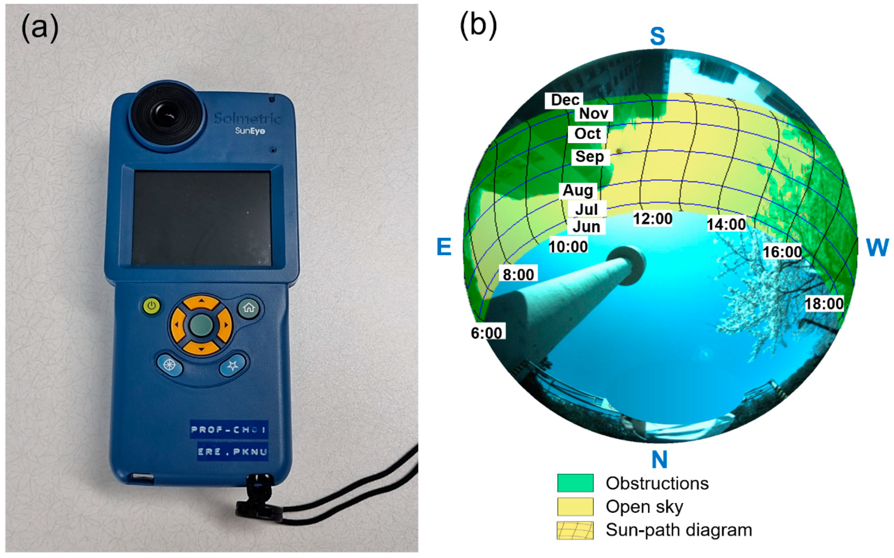
Figure 3.
The process of measuring the maximum power point of a solar PV module. (a) The PV analyzer was produced by Solmetric. (b) The 50 W solar PV module. (c) Example of the I–V and P–V curves.
Figure 3.
The process of measuring the maximum power point of a solar PV module. (a) The PV analyzer was produced by Solmetric. (b) The 50 W solar PV module. (c) Example of the I–V and P–V curves.
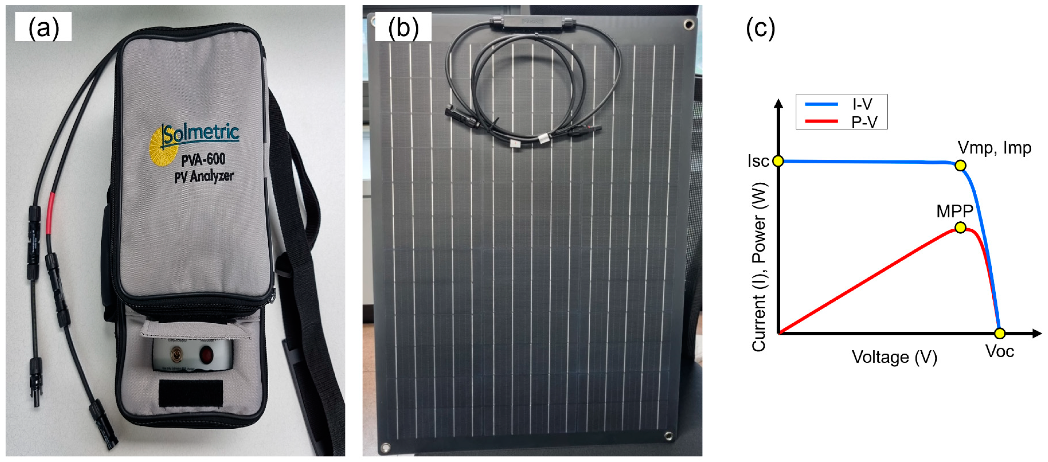
Figure 4.
Photograph describing the experiment setting. (a) The seven survey points in the parking lot. (b) A solar PV module was placed on the car roof with a PV analyzer connected to the PV module. (c) A laptop PC was used to wirelessly control the PV Analyzer and record the data.
Figure 4.
Photograph describing the experiment setting. (a) The seven survey points in the parking lot. (b) A solar PV module was placed on the car roof with a PV analyzer connected to the PV module. (c) A laptop PC was used to wirelessly control the PV Analyzer and record the data.
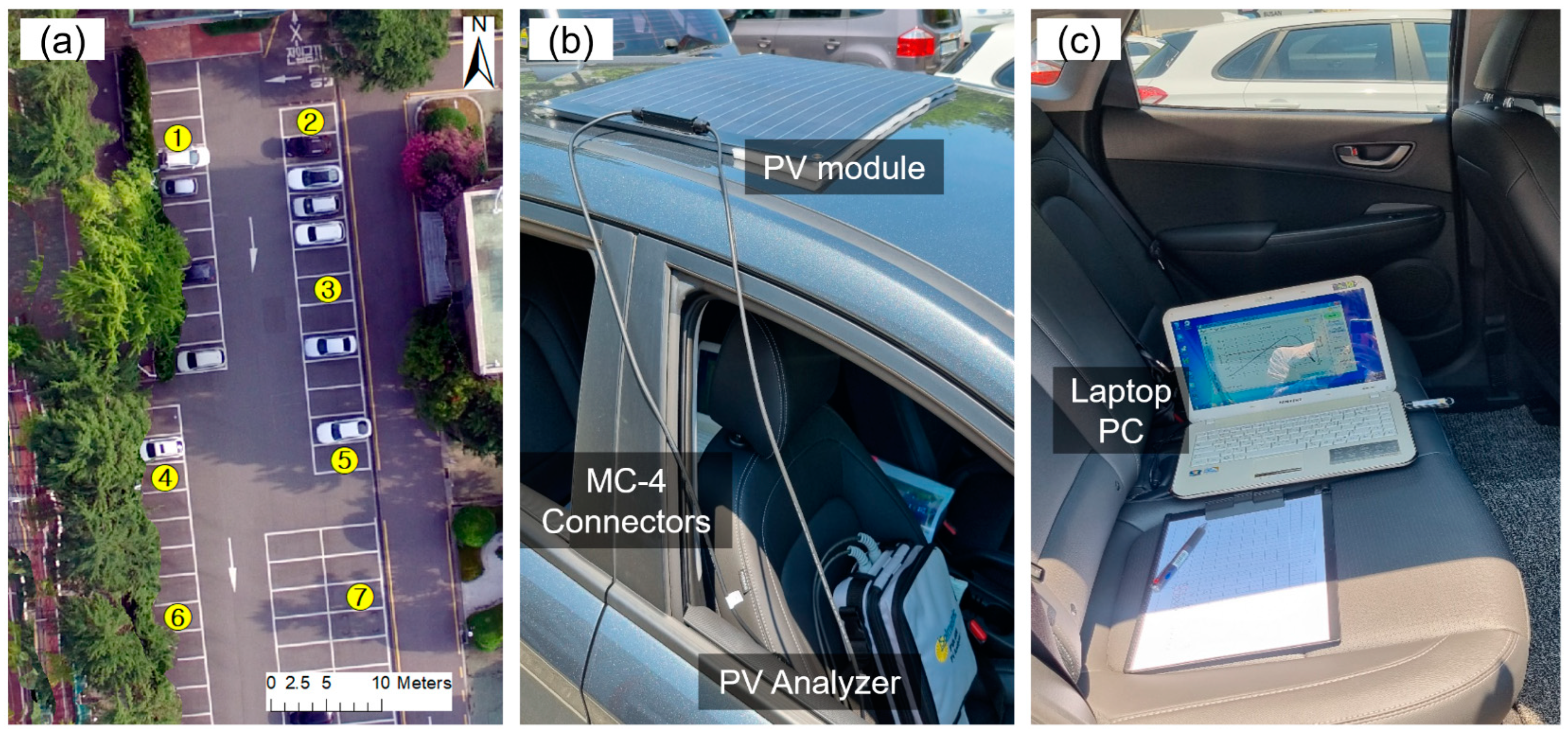
Figure 5.
Fisheye images overlaid with the sun-path diagram. The results at: (a) survey point 1; (b) survey point 2; (c) survey point 3; (d) survey point 4; (e) survey point 5; (f) survey point 6; and (g) survey point 7.
Figure 5.
Fisheye images overlaid with the sun-path diagram. The results at: (a) survey point 1; (b) survey point 2; (c) survey point 3; (d) survey point 4; (e) survey point 5; (f) survey point 6; and (g) survey point 7.
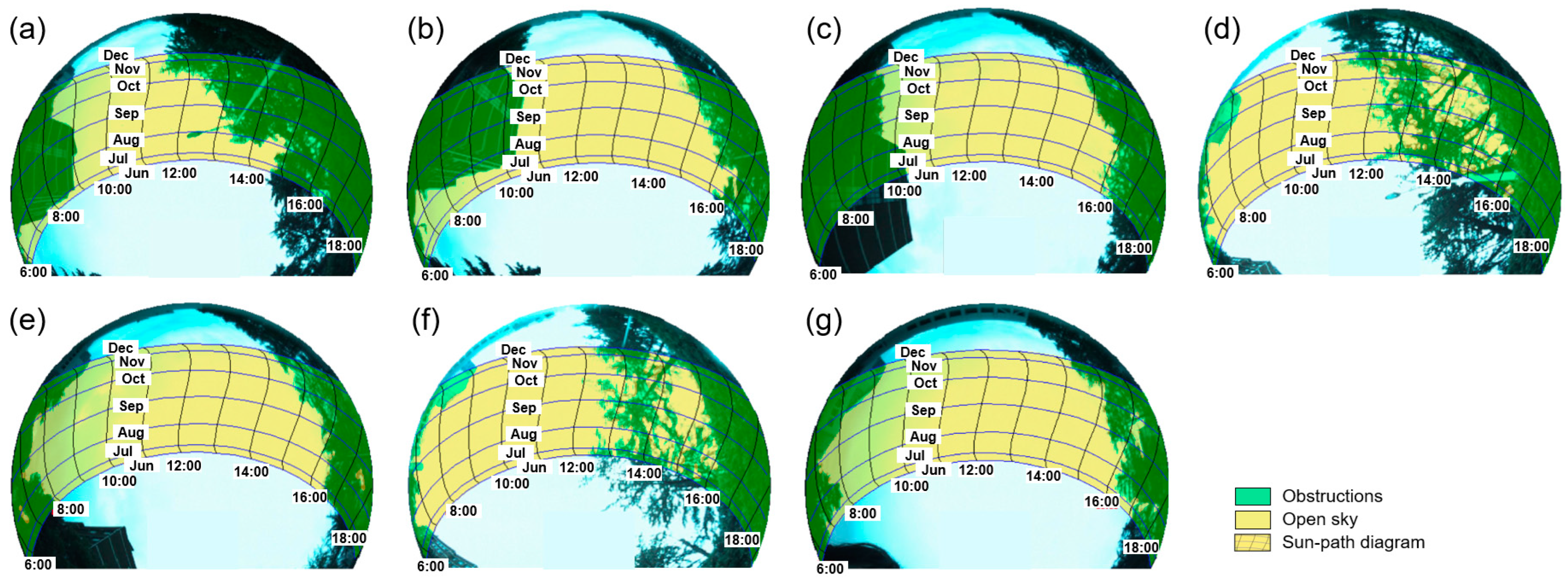
Figure 6.
Shading matrices generated using fisheye images and sun-path diagrams. (a) Survey point 1; (b) survey point 2; (c) survey point 3; (d) survey point 4; (e) survey point 5; (f) survey point 6; and (g) survey point 7.
Figure 6.
Shading matrices generated using fisheye images and sun-path diagrams. (a) Survey point 1; (b) survey point 2; (c) survey point 3; (d) survey point 4; (e) survey point 5; (f) survey point 6; and (g) survey point 7.
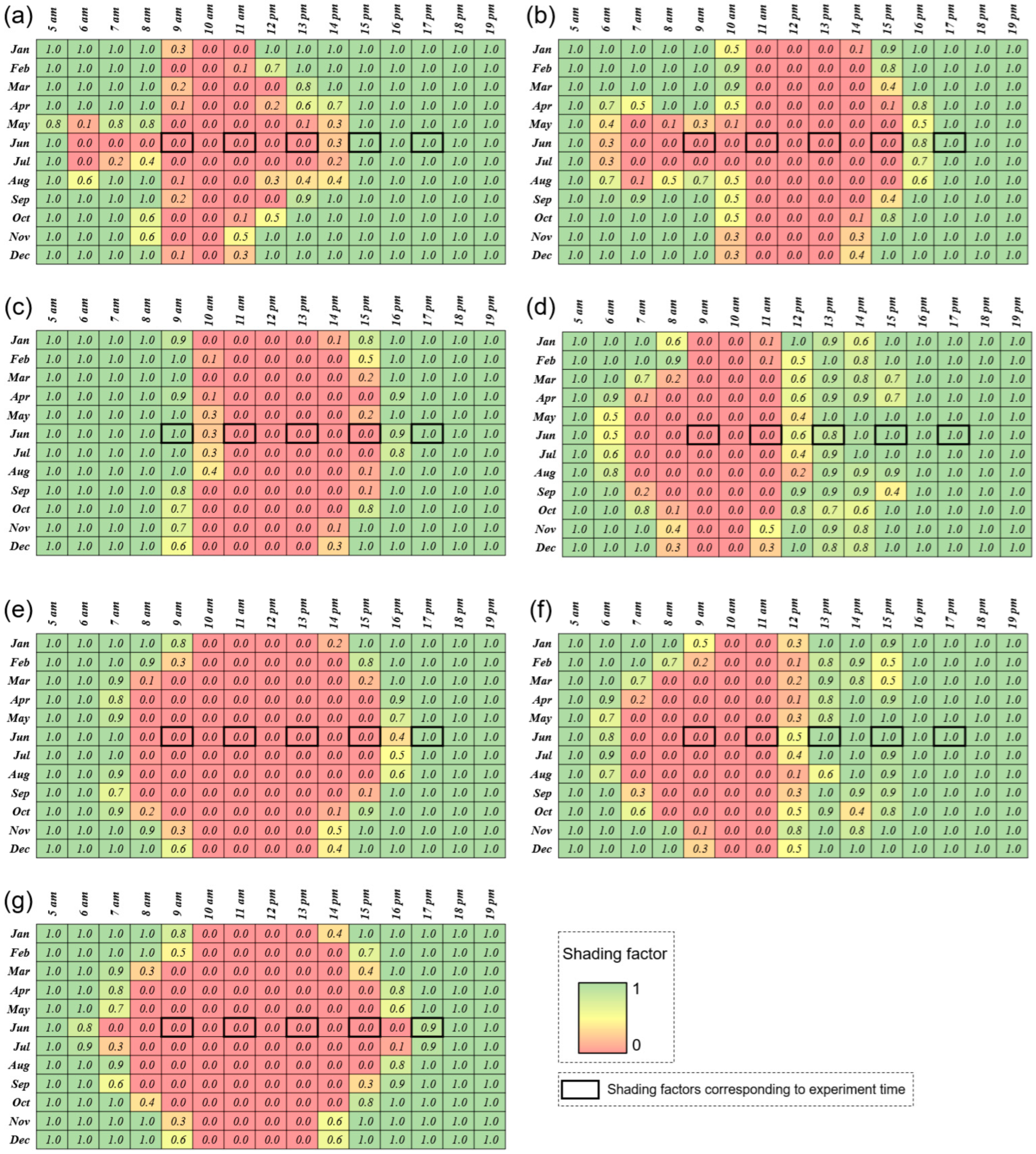
Figure 7.
The PV modules at survey point 4 (a) without any shadows at 11 a.m. and (b) partially shaded by trees at 13 p.m.
Figure 7.
The PV modules at survey point 4 (a) without any shadows at 11 a.m. and (b) partially shaded by trees at 13 p.m.
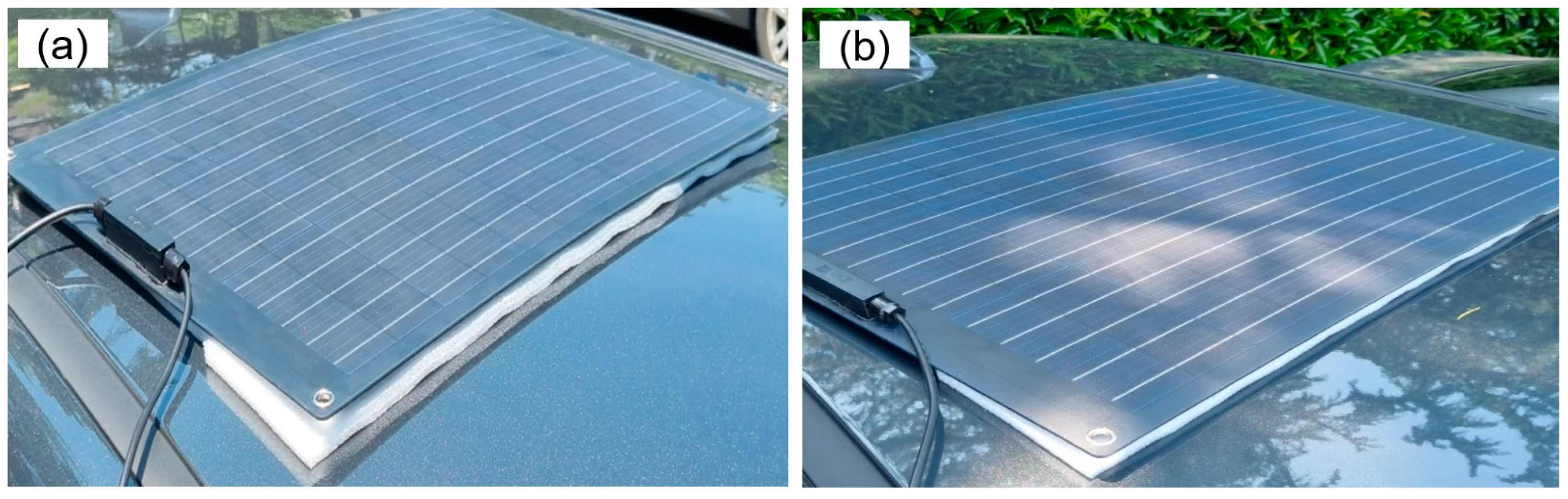
Figure 8.
The shading factor and mean maximum power point (MPP) results at 9 a.m. A graduated symbol map representing the shading factor and maximum power point of the seven survey points. Inner and outer circles provide the shading factor and MPP, respectively.
Figure 8.
The shading factor and mean maximum power point (MPP) results at 9 a.m. A graduated symbol map representing the shading factor and maximum power point of the seven survey points. Inner and outer circles provide the shading factor and MPP, respectively.
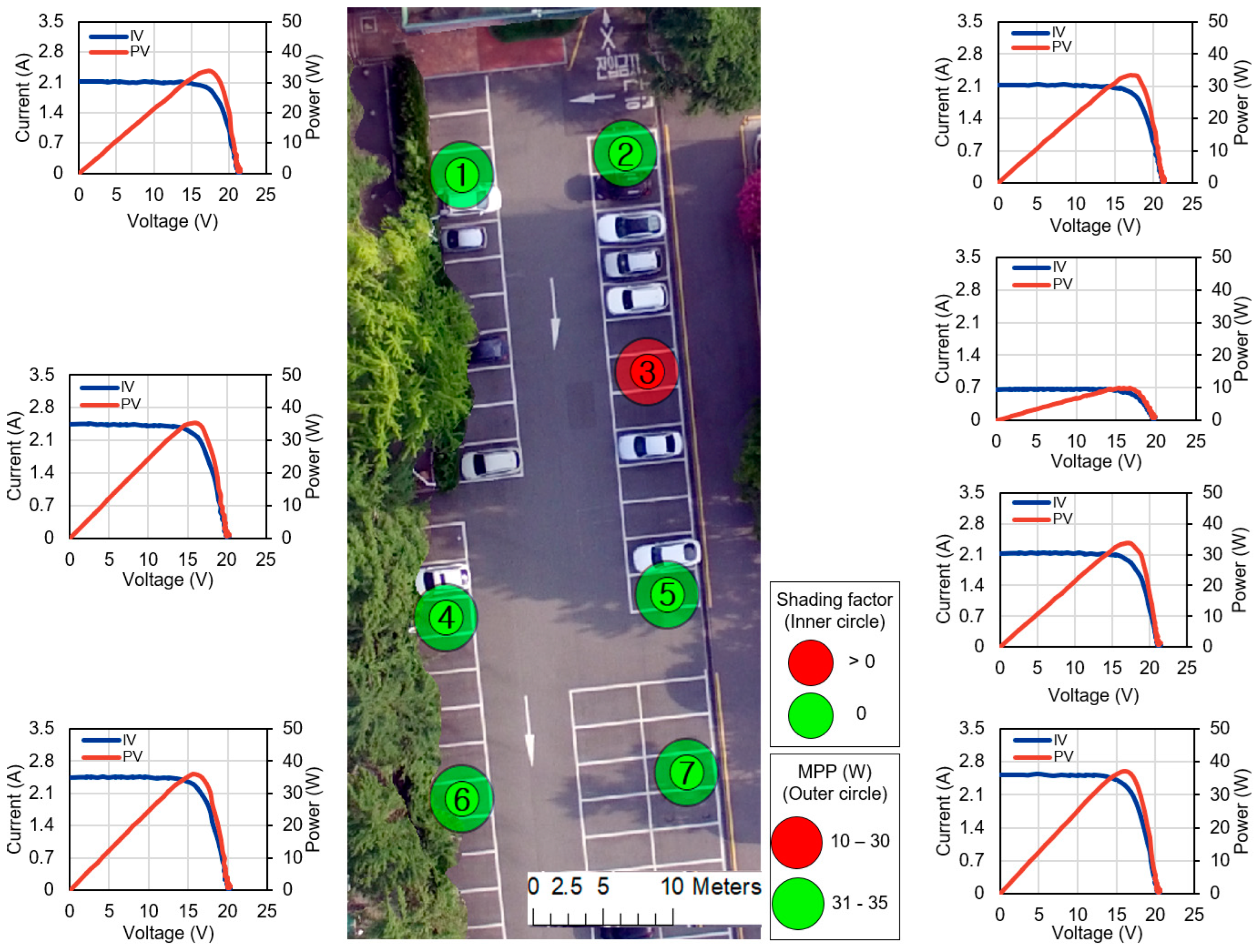
Figure 9.
The shading factor and mean maximum power point (MPP) results at 11 a.m.
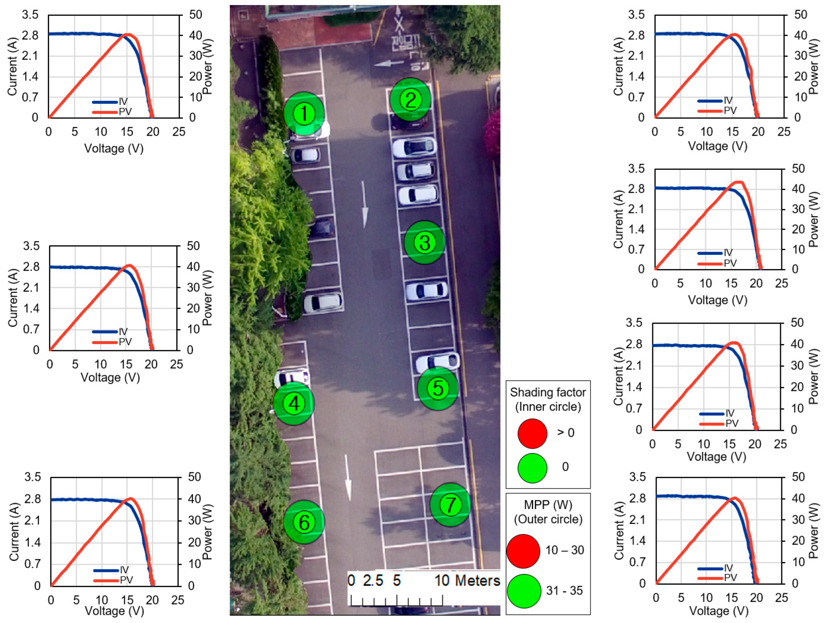
Figure 10.
Results of the shading factor and mean maximum power point (MPP) at 13 p.m.
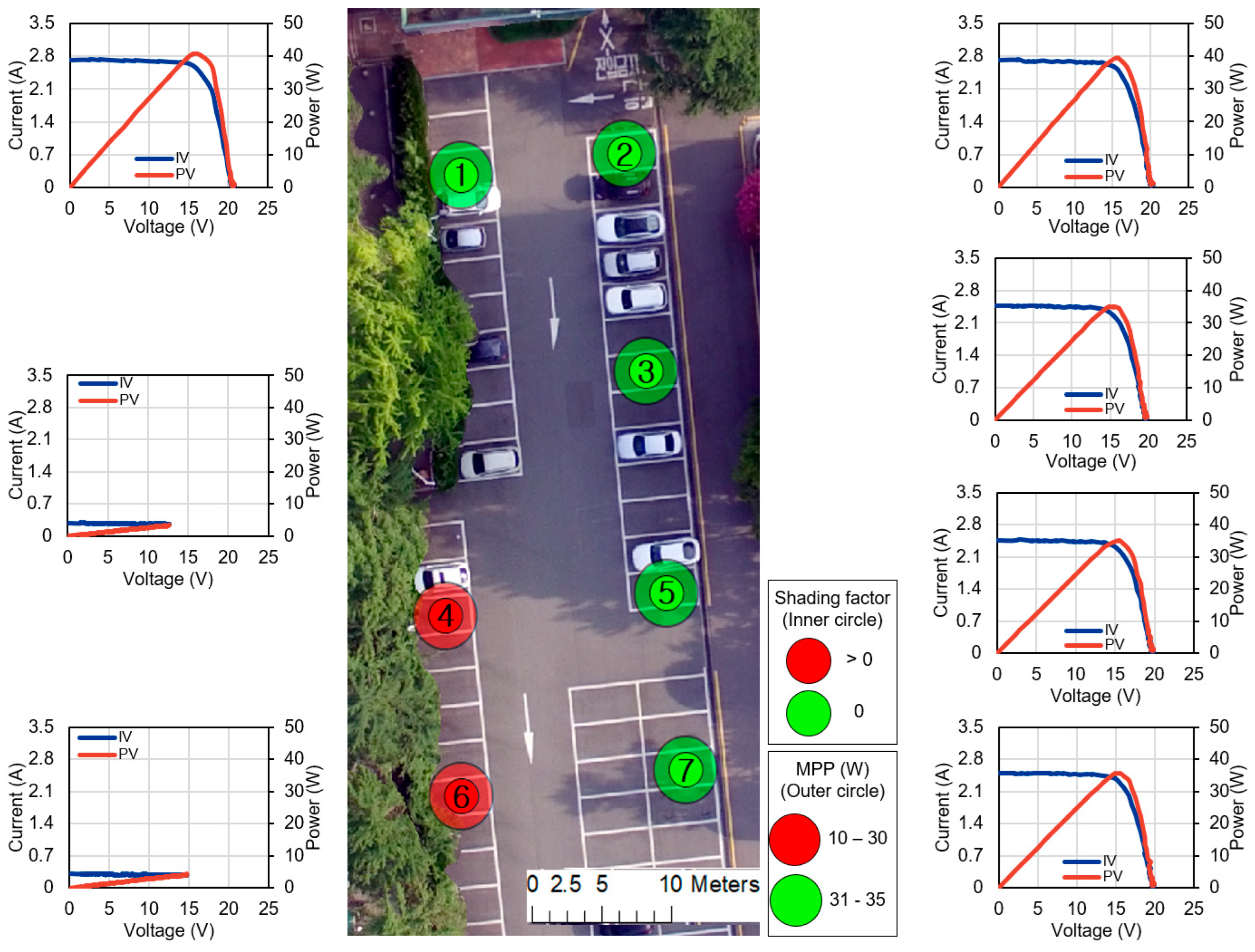
Figure 11.
Results of the shading factor and mean maximum power point (MPP) at 15 p.m.
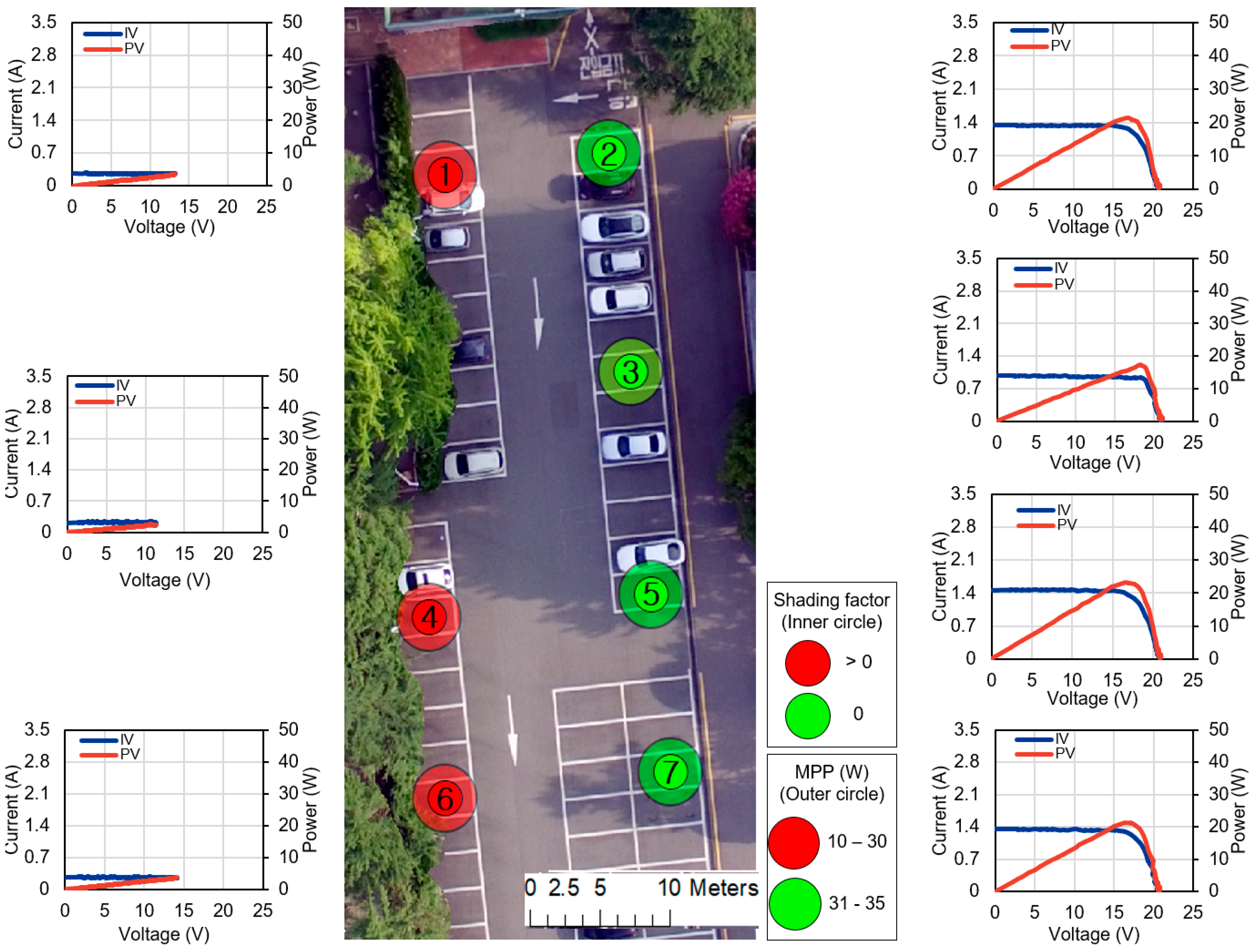
Figure 12.
Results of measuring the shading factor and mean maximum power point (MPP) at 17 p.m.
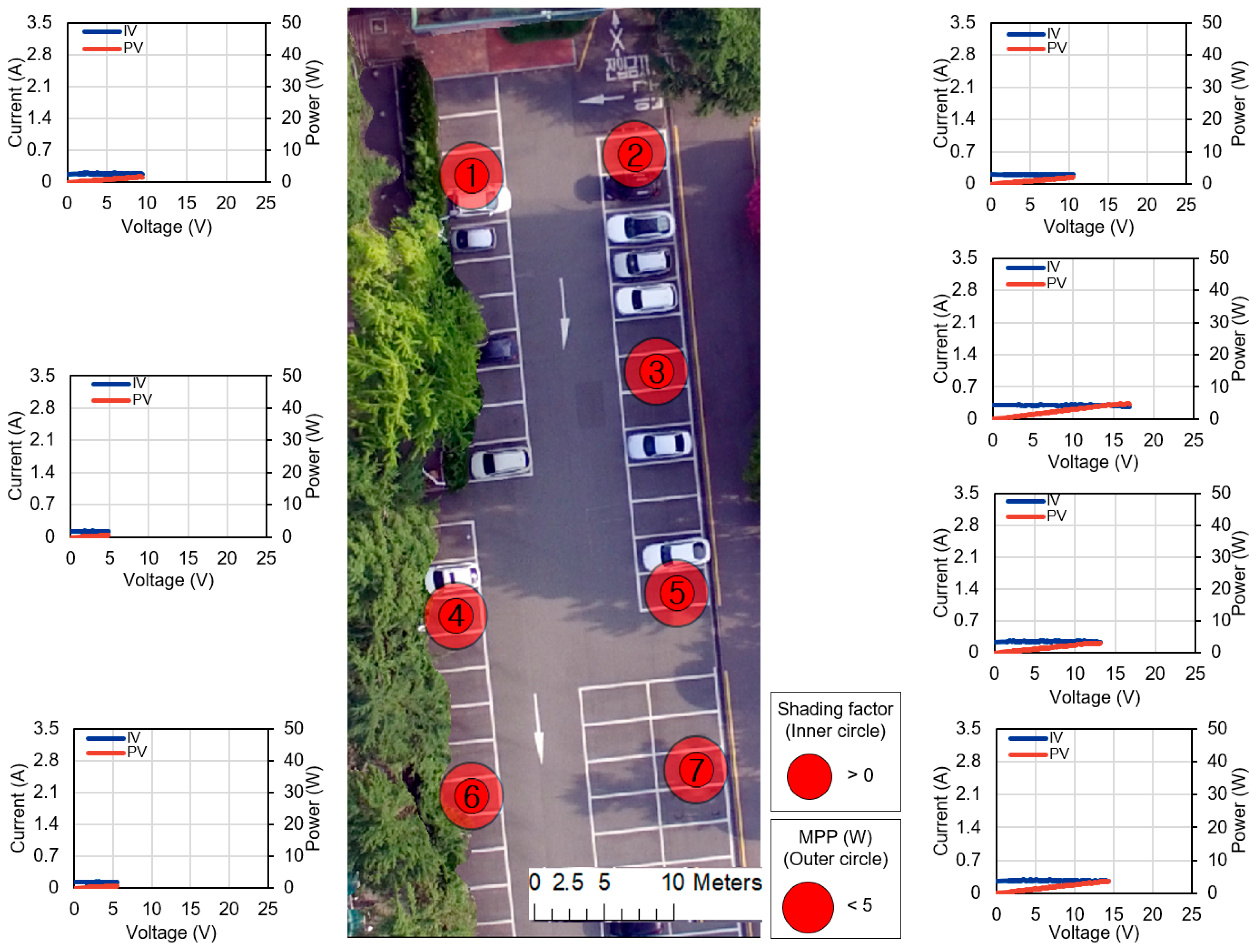
Figure 13.
Comparison of the shading factor and mean maximum power point for each time of (a) 9 a.m., (b) 11 a.m., (c) 13 p.m., (d) 15 p.m., and (e) 17 p.m.
Figure 13.
Comparison of the shading factor and mean maximum power point for each time of (a) 9 a.m., (b) 11 a.m., (c) 13 p.m., (d) 15 p.m., and (e) 17 p.m.
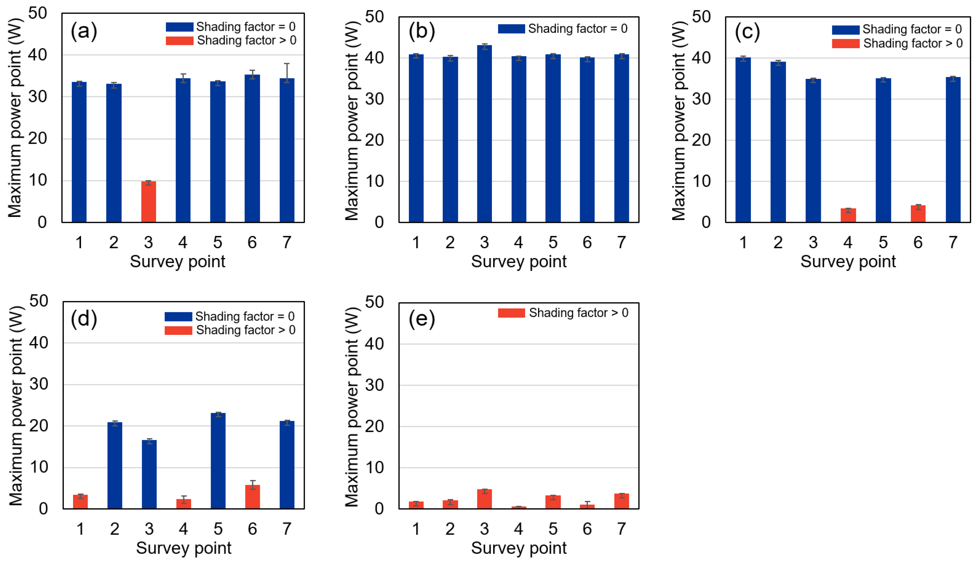
Figure 14.
Mean shading factors (%) calculated for seven survey points in June.

Table 1.
Specifications of the PV Analyzer produced by Solmetric used in the experiment.
| Parameter | Specification |
|---|---|
| Current measurement range | 0–20 A dc |
| Voltage measurement range (Voc) | 20–600 V dc |
| Load type | Capacitive (3 capacitance values) |
| Measurement sweep time | 50–240 ms |
| Measurement points per trace | 100 |
| Wireless communication range | 10 m |
Table 2.
Specifications of the PV module used in the experiment.
| Parameter | Specification |
|---|---|
| Model | QH50M-18PP |
| Dimension | 720 × 515 × 2.8 mm |
| Power at the maximum power point (MPP) | 50 W |
| Voltage at the maximum power point (Vmp) | 18 V |
| Current at the maximum power point (Imp) | 2.78 A |
| Open-circuit voltage (Voc) | 21.24 V |
| Short-circuit current (Isc) | 3.06 A |
| Max system voltage | 500 V |
| Test condition | AM = 1.5, E = 1000 W/m2, Tcell = 25 °C |
Table 3.
Solar insolation results from each time point collected from the study area (18 June 2022).
Table 3.
Solar insolation results from each time point collected from the study area (18 June 2022).
| Experiment Time | 9 a.m. | 11 a.m. | 13 p.m. | 15 p.m. | 17 p.m. |
|---|---|---|---|---|---|
| Insolation (W/m2) | 261.89 | 750.03 | 721.74 | 453.56 | 125.08 |
Table 4.
Shading factors over time at each survey point.
| No. of Survey Point | Shading Factor | ||||
|---|---|---|---|---|---|
| 9 a.m. | 11 a.m. | 13 p.m. | 15 p.m. | 17 p.m. | |
| 1 | 0 | 0 | 0 | 1 | 1 |
| 2 | 0 | 0 | 0 | 0 | 1 |
| 3 | 1 | 0 | 0 | 0 | 1 |
| 4 | 0 | 0 | 0.8 | 1 | 1 |
| 5 | 0 | 0 | 0 | 0 | 1 |
| 6 | 0 | 0 | 1 | 1 | 1 |
| 7 | 0 | 0 | 0 | 0 | 0.9 |
Publisher’s Note: MDPI stays neutral with regard to jurisdictional claims in published maps and institutional affiliations. |
© 2022 by the authors. Licensee MDPI, Basel, Switzerland. This article is an open access article distributed under the terms and conditions of the Creative Commons Attribution (CC BY) license (https://creativecommons.org/licenses/by/4.0/).
Share and Cite
MDPI and ACS Style
Baek, J.; Choi, Y. An Experimental Study on Performance Evaluation of Shading Matrix to Select Optimal Parking Space for Solar-Powered Electric Vehicles. Sustainability 2022, 14, 14922. https://doi.org/10.3390/su142214922
AMA Style
Baek J, Choi Y. An Experimental Study on Performance Evaluation of Shading Matrix to Select Optimal Parking Space for Solar-Powered Electric Vehicles. Sustainability. 2022; 14(22):14922. https://doi.org/10.3390/su142214922
Chicago/Turabian StyleBaek, Jieun, and Yosoon Choi. 2022. "An Experimental Study on Performance Evaluation of Shading Matrix to Select Optimal Parking Space for Solar-Powered Electric Vehicles" Sustainability 14, no. 22: 14922. https://doi.org/10.3390/su142214922
Note that from the first issue of 2016, this journal uses article numbers instead of page numbers. See further details here.