Mathematical Modelling of Biogas Production in a Controlled Landfill: Characterization, Valorization Study and Energy Potential

Abstract

Methane potential is the volume of methane gas produced during anaerobic degradation in the presence of the bacteria of an initially inserted sample. This paper presents a degradation study of the green and industrial fermentable waste sheltered by the landfill of Mohammedia in which the biogas deposit and the associated recoverable energy at the end of exploitation is estimated and the power of the gas engine of the proposed cogeneration unit is calculated. The Total potential biogas production value of the household waste of the city of Mohammedia is much higher than that of the American and French household waste recommended by the US EPA and French ADEME. This calls into question the adaptability of the modeling tools for biogas production to Moroccan waste. The four modeling equations for landfill will be evaluated. The results show that the ADEME model proved to be more descriptive and better adapted to this case.

1. Statement of Novelty

The recuperation of biogas from the Mohammedia site landfill was calculated utilizing four demonstrating conditions, and the present models included only family waste, with methanogenic potential estimations of 100 m³ to 170 m³ of CH₄/ton of waste for the American models and 50 out of 100 for the French ADEME model. To adjust to the Moroccan setting, and especially to the instance of Mohammedia, we extrapolated a lot of information on waste from various regions and enterprises so as to get values depicting the methanogenic potential specific to the various substrates. This permitted us to gauge the biogas deposit indicated by the given operating horizon.

2. Introduction

Landfill is an easy to implement and relatively inexpensive waste disposal technique. Without proper management, however, it can lead to a variety of hygienic, health and environmental problems. Only a landfill that has been stabilized, and is therefore without further development, can be defined as no longer being harmful to the environment. When it comes to renewable energies, wind turbines, solar collectors and hydropower are most often mentioned. However, there are other solutions, such as energy production from biomass: wood, biofuels or biogas [1]. The population of developing countries is growing, leading to an increase in the needs of the poor and the production of waste and effluents. Waste recycling contributes to poverty alleviation and environmental sanitation [2].

Mechanization is an anaerobic digestion process that generally achieves double the energy yield of the original process. The objective of energy recovery by methane (CH₄) is the recovery and stabilisation of organic waste with a view to material recovery by its partial restitution to the ground [3,4]. With ever-increasing and more diversified consumption all over the world, waste production is constantly increasing in quantity and quality, thus creating enormous risks to the environment and both the safety and health of local populations [3]. Landfilling remains the predominant method of disposal of household and similar waste in Africa, particularly in Morocco, in part because of its simplicity, but also because of its lower cost compared with other methods, such as incineration.

The Mohammedia control landfill receives a significant amount of waste with high methanogenic potential every day, such as household waste (61% organic matter), green waste, poultry droppings and tannery waste. By anaerobic decomposition, this mixture generates a good quality biogas (CH₄ 55.6%, CO₂ 32%, H₂S 600 ppm, O₂ 1%) which reminds us of its value in other applications [3]. This study was carried out in order to quantify the biogas deposit at the Mohammedia site using four modelling equations, these models using only household waste, with methanogenic potential values in the order of 100 m³ to 170 m³ of CH₄/tonne of waste for the American models [5] and 50 of 100 for the French ADEME model [6], corresponding to the specificities of the waste and the regions where these tools were developed [7]. In order to adapt them to the Moroccan context, in particular to the case of Mohammedia, we extrapolated a heap of data on waste from different municipalities and industries in order to obtain values describing the methanogen potential specific to the different substrates. This allowed us to estimate the biogas deposit according to the given operating horizon.

3. Description of the Studied Zone

The Mohammedia interprovincial control landfill is located in the municipality of Ben Yakhlef, on the shoreline. It is west of Chaaba el Hamra, a tributary of the west bank of the Nfifikh river, about 270 m south of the Dayat Al Hila security perimeter (X = 32440, Y = 338979) and occupies an area of 47 hectares.

The zone is moderately hilly and ends at the edge of the west bank of a talweg (Chaaba El Hamra) perpendicular to the west bank of Oued Nfifikh. From upstream to downstream, the site has a height difference of 27 m. Its proximity to the ocean gives this region a temperate and humid climate (80% humidity) with a mild winter and a summer cooled by the ocean breezes. The average temperature is 23 °C and the annual precipitation level is 400 mm, in addition to a daily evapotranspiration potential of 5–6 mm/12 h. Eleven rural and urban municipalities (including Mohammedia, Ain Harrouda, Bouznika, Ben Sliman, El Mansouria, Ech-Challalat, Ben Yakhlaf, Sidi Mousa ben ali and Sidi Mousa El Majdoub) are served by the so-called landfill centre, which started in 2012 and is scheduled to close in 2032. The project area is divided between the landfill area and other landfill accessories, as described in the plan below, which shows the biogas collection network of crates 1 and 2, already in operation [8].

4. Materials and Methods

4.1. Experimental Design

In order to measure the amount of biogas produced by the waste studied, an anaerobic digestion device and a device for determining the volume of biogas generated by water displacement were established in the laboratory. A mass of 20 g of each sample was crushed and mixed with 100 mL of water and incubated for 40 days in a bioreactor placed in a water bath at a constant temperature (35 °C), promoting bio-mechanisation (Figure 1) [9].

4.2. Modeling Equations

4.2.1. EPA Model

The US EPA (Environmental Protection Agency) has also carried out a study; this led to a model based on data collected on site. This Model is based on a first-order Equation (1) with a decreasing generation rate of biogas over time [10,11]:

$$Qt=\mathbf{2}\times L_{\mathbf{0}}\times R\left( e^{\left(-KC\right)}-e^{\left(-Kt\right)}\right)$$

(1)

Qt: quantity of biogas generated over time t (m³/year);

L₀: total potential biogas production (m³ CH₄/t of waste);

K: kinetic constant for biogas generation (year⁻¹);

T: time elapsed since storage began (year);

R: average rate of waste accepted during the site’s operating period (t/year);

C: time since site closure (C = 0 year for active sites) (year).

$$L_{\mathbf{0}}=FCM. COD. CODF.A.\frac{\mathbf{16}}{\mathbf{12}} . \mathbf{1000}$$

(2)

FCM: correction factor of the CH₄, expressed as a percentage;

COD: degradable organic carbon, expressed as t of C/t of waste;

CODF: concealed COD fraction;

A: fraction of CH₄ in biogas;

16/12: stoichiometry coefficient.

$$COD=\mathbf{0.4}E+\mathbf{0.17}F+\mathbf{0.15}G+\mathbf{0.3}H$$

(3)

E: fraction of waste consisting of paper and textiles;

F: fraction of waste consisting of garden and/or park waste;

G: fraction of waste consisting of food waste;

H: fraction of waste consisting of wood and/or straw.

4.2.2. LANDGEM Model

The LANDGEM model is based on a first-order degradation equation that is estimated over several years. Indeed, for a mass of waste accepted in year i (Mi), methane production follows a decreasing exponential law. For several years, production is evaluated every tenth of a year. The equation used to estimate the total amount of methane produced in a TEC is [12,13]:

$$Q\left(C{H}_{\mathbf{4}}\right)={\displaystyle \sum }_{i=\mathbf{1}}^n{\displaystyle \sum }_{j=\mathbf{0.1}}K L_{\mathbf{0} }\frac{M_i}{\mathbf{10}} e^{\left(-K{t}_{ij}\right)}$$

(4)

i: time increment of 1 year;

j: cutting the year into tenths.

4.2.3. ADEME Model

ADEME estimates the methane emissions from the TECs by calculating the quantity of methane produced (uncaptured methane and captured methane) using this expressions [14,15]

$$Q\left(CH\mathbf{4}\right)={{\displaystyle \sum }}^{\hspace{1em}}{L}_{\mathbf{0} }{\displaystyle \sum }_{i=\mathbf{1}}^{\mathbf{3}}{A}_i{P}_i{K}_i{e}^{\left(-K_i\left(t-x\right)\right)}$$

(5)

$$L_{\mathbf{0}}=\mathbf{0.934}.C_{\mathbf{0}}\left(\mathbf{0.014}.T+\mathbf{0.28}\right) en\frac{m^{\mathbf{3}}}{t}$$

(6)

i: the subdivision into three categories of waste;

P_i: the fraction of waste with degradation constant i;

C₀: biodegradable organic carbon;

T: degradation temperature 30 °C;

A_i: factor of the mass of waste accepted in year i;

x: year of landfilling of waste.

The three degradation constants K depend on the biodegradability of the waste:

K₁ = 0.5 in order to degrade 15% of waste (easily biodegradable);

K₂ = 0.10 in order to degrade 55% of waste (moderately biodegradable);

K₃ = 0.04 in order to degrade 30% of waste (poorly biodegradable);

The degradation kinetics are assumed to be the same regardless of the composition of the waste [16].

4.2.4. Scholl Canyon Model

The Scholl Canyon Model is a first-order decomposition model. It allows the calculation of CH₄ resulting from the decomposition of waste, taking into account the fact that this waste decomposes over many years. It is expressed in Equation (6) [17]:

$$Qt={{\displaystyle \sum }}^{\hspace{1em}}(K L_{\mathbf{0} }{M}_x \left( e^{\left(-K\left( t-x\right)\right)}\right) )$$

(7)

Qt: quantity of methane produced during the year in question (T) (kg of CH₄/year);

x: year of entry of the waste;

M_x: amount of waste landfilled during the year × (Mt);

L₀: methane production potential (kg of CH₄/t of waste);

T: considered year.

4.3. Sampling and Analysis

The samplings were made in Tedlar bags and glass ampules. The H₂ and N₂ were analyzed by chromatography on a molecular sieve using a detector with thermal conductivity. The CH₄ and CO₂ were measured by porous polymer analysis with a thermal conductivity detector (TCD). The C₂ to C₅ were analyzed by chromatography on a porous polymer with a flame ionization detector (FID). The CO was analyzed using the non-dispersive infrared technique.

5. Results and Discussion

5.1. Tonnage of Waste

The Mohammedia controlled landfill receives on average 500 t/d of DMA that constitutes 74% of the total tonnage of various types (

Table 1. Percentage by type of waste.

Designation	Value (t/d)	%
Household garbage	387	70%
Green waste	5	1%
Household garbage, soil and rubble	100	18%
Non-hazardous industrial waste	64	11%

): household waste (OM); green waste; mixtures of household waste, soil and gravel; and common industrial waste considered to be AMD.

Among the wastes with high methanogenic potential destined for landfill are DM, green waste and two types of industrial waste, namely: waste from the Mohammedia tannery and poultry droppings brought in by the Delicate-meat company. The two graphs that follow show the tonnage of this waste since the landfill opened (Figure 2 and Figure 3).

5.2. Waste Characterization

The studies on the characterization of household and similar waste in the city of Mohammedia conducted by A. Ouatmane in 2018 and A. El Maguiri et al. in 2016 [7,8,9] report that the fraction is <80 mm, which represents fermentable organic matter in the order of 61%. However, the >80 mm fraction can be divided into categories and sub-categories, as shown in Figure 4.

Bi-monthly sampling of the same landfill waste pile showed (

Table 2. Results of physicochemical analyses of the waste fraction <80 mm.

Description	Unit	Value
Density: fraction < 80 mm	t/m3	1.09
Humidity	%	38.02
Organic matter	g/100 g MS	69.93
Total organic carbon	g/100 g MS	40.26
Nitrogen	g/100 g MS	1.25
Report C/N	-	32.21
PCI fraction < 80 mm	Kcal/Kg	1002
PCI fraction > 80 mm	Kcal/Kg	2071

) a clear evolution in the physical and chemical parameters during the landfilling of the waste, in particular a significant decrease in the organic carbon content due to mineralisation. The total nitrogen content showed a significant increase during fermentation. This variation corresponds in fact to a relative enrichment in nitrogen of the residual dry matter of the compost, the total amount of nitrogen actually decreasing as illustrated. The mineral nitrogen contents are always low, and their evolution is typical of what is found in compost heaps with a low level of ammoniac nitrogen and traces of nitrate, which then forms nitrate at the end of maturation. This maturation results in a lowering of the C/N ratio from 32, indicating a stabilisation of the organic compounds. Similarly, the equivalent humidity of the product falls, this last point being related to the concomitant rise in pH. Table 2 shows the results of the physicochemical analyses carried out during the DMA characterization.

All the results are presented in Table 2. Total organic carbon corresponds to approximately 40% of the dry matter of the composts analyzed. Given the very heterogeneous composition of these materials and the diversity of their origins, we can assume that the variations observed were moderate (

Table 3. TOC value in g/100 g [3,4].

Type of Waste	TOC (g/100 g)	C/N
Household waste	40.26 [2]	32.21
Green waste	27 [3]	55
Poultry droppings	13.59 [4]	3.68
Tannery waste	14 [4]	3

).

The C/N ratio is around 32.21 at the beginning of the first phase of the process. Subsequently, a decrease in this ratio is noted, which becomes equal to 28 at the end of the first phase. This reduction is explained by the active transformation of the carbon into carbon dioxide, accompanied by a decrease in the content of organic acids in the waste mass. The purpose of this input is to amplify the microbial activity to prepare for the start of the next stage.

5.3. Methanogenic Potential

The potential for biogas generation by anaerobic decomposition of the various fermentable wastes sheltered by the TEC is a critical parameter for modelling biogas production. The US EPA recommends L0 values ranging from 170 m³ of CH₄ per tonne of waste for arid areas to 96 m³ for wetlands [17,18], though these values take into consideration the composition and physicochemical properties of household waste in the United States, which are certainly different from those in Morocco (

Table 4. Table of COD and L0 calculation results.

	COT (g/100 g)	COD	FCM	CS	F (%)	L0 M3/t
Household waste	40.26	0.099	1	1.333	55.6	563.77
Green waste	27	0.37	1	1.333	65 [18]	1649.77
Poultry droppings	13.59	0.542	1	1.333	60 [18]	1124.23
Tannery waste	14	0.3	1	1.333	60 [18]	640.24

).

Equation (2) includes in its expression three key elements (TOC, COD and F) that define the methanogenic potential of waste. The first expresses the carbon content, an essential element in the formation of methane. The term COD (3) relates the composition of waste, and knowing the composition and physical and chemical properties of its waste enables the calculation of L0 specific to a region.

The estimate of L0 using Equation (6) of the ADEME model gives a value of 26.3 m³/t. Compared with the values recommended by the EPA and LANDGEM, this is extremely small and does not reflect the methanogenic potential of Mohammedia household waste (Figure 5), whose fermentable organic matter fraction is around 61% [6], which is probably significant compared with the % MO of waste in France and the US.

After 40 days of fermentation of the different substrates at a temperature of 35 °C, the graph of the biogas production kinetics, which is strongly related to temperature and C/N ratio [7], shows that poultry droppings produce the largest volume of biogas (266 mL), which is certainly due to the abundance of lipids in the substrate. Then come in decreasing order green waste, tannery waste and household waste, with respective volumes of 189 mL, 160 mL and 150 mL.

These experimental results do not coincide at all with the empirically calculated values of L0 since this series of experiments is limited in time to 40 days, while the methanogenic potential calculation equation given by the US EPA takes into account the total consumption of the substrate.

In addition, the monitoring of the quality of biogas generated for all samples shows that the oxygen content increases from 19%/V to 7%/V during the first week, with carbon dioxide production averaging 5%/V. However, methane only appeared during the last week in insignificant quantities ranging from 1% to 2% by volume.

5.4. Biogas Production Modelling via the Four Models

The different modelling equations mentioned in this work utilize three terms (tonnage, K and L0) that define the volume of biogas/methane generated in a time interval.

The methane generation constant (K) represents the decomposition rate. This depends mainly on waste and precipitation on site. High levels of K indicate a higher level of gas production over time [7]. As with L0, the US EPA has set values of K ranging from 0.02 year⁻¹ to 0.7 year⁻¹ for arid and humid areas respectively, as well as a conventional value of 0.05 year⁻¹ [19].

The French model developed by ADEME, on the other hand, uses three degradation constants K according to the biodegradability of the waste:

K₁ = 0.5 (easily biodegradable);

K₂ = 0.10 (moderately biodegradable);

K₃ = 0.04 (poorly biodegradable).

The values of the methane generation constant adopted by ADEME are somewhat higher than those of the American models. However, due to the high humidity content of the waste and the climatological conditions characterizing the study area, the ADEME model is the most suitable for modelling biogas production for waste from the city of Mohammedia (Figure 6). In addition, it offers the possibility of modelling methane production for waste of a different nature, which is the case in this study, by summing the L0i and Ki for n substrates (Equation (5)).

In this study, we assigned values of K to the different types of waste studied (0.1 for household waste, 0.5 for green waste and 0.04 for poultry droppings and tannery waste) according to their degree of biodegradability by comparing the carbon/nitrogen ratios.

The modelling results show only a slight variation between three of the models, the EPA, SCHOLL CANYON and ADEME, but the LANDGEM model showed a significant difference compared with the others, which is why production is evaluated on a tenth of a year basis [20].

Details of the calculations are provided in Appendix A.

5.5. Estimate of the Biogas Field

The estimation of the tonnage of household waste from the different urban and rural municipalities between 2018 and 2032, according to their respective waste production ratios of 0.76 and 0.3 Kg/inhab/d [19], begins with the calculation of the population evolution and the ratio using Equations (8)–(10) (Appendix B).

$$EP=Ai\times {\left(\mathbf{1}-\frac{rate of increase}{\mathbf{100}}\right)}^{Ai-A\mathbf{0}}$$

(8)

$$ER=\mathbf{0.76}\left(ou \mathbf{0.3}\right)\times {\left(\mathbf{1}+\mathbf{1.36}/\mathbf{100}\right)}^{Ai-A\mathbf{0}}$$

(9)

$$T=\left(population\times ratio\times \mathbf{365} /\mathbf{1000}\right)$$

(10)

EP: population evolution;

ER: ratio evolution;

T: annual tonnage;

Ai: population i.

In view of the difficulty of estimating the tonnage of green and industrial waste, the average percentages of the apparent tonnage recorded between 2012 and 2018 of each substrate and their percentages of contribution to methane production were used to predict the tonnage of fermentable waste until the end of operation, including the volume of biogas related to it (Figure 7).

The calculation of greenhouse gas emissions is performed using Equation (11) below:

$$GH G_p=\mathbf{21}\left(\mathbf{0.016}\times \frac{Q_p}{\mathbf{22.4}}\right)$$

(11)

GHG_p: equivalent CO₂ emissions (t CO₂/year);

Q_p: quantity of methane produced (m³/year);

21: ratio of CH₄ to 1 CO_2.

Table 5. Calculation results for the annual production of biogas, CH₄ and CO₂ equivalent.

Year	Tonnage DM	Tonnage (DM, DV, FV, DT)	Biogas	CH4	GHGp
Unit	MKg/Years	MKg/Years	MM3/Years	MM3/Years	KT CO2/Year
2012	103.88	114.27	10.64	5.92	88.75
2013	138.26	152.09	14.60	8.12	121.81
2014	26.35	28.99	2.863	1.59	23.88
2015	146.72	161.40	16.81	9.34	140.19
2016	138.23	152.05	14.68	8.16	122.44
2017	144.72	159.19	15.62	8.67	130.34
2018	161.96	178.15	16.48	9.16	137.47
2019	101.27	111.40	9.29	5.17	77.49
2020	101.60	111.76	9.32	5.18	77.74
2021	101.93	112.12	9.35	5.20	78.00
2022	102.26	112.49	9.38	5.21	78.25
2023	102.59	112.85	9.41	5.23	78.50
2024	102.93	113.22	9.44	5.25	78.76
2025	103.26	113.59	9.47	5.27	79.01
2026	103.60	113.96	9.50	5.28	79.27
2027	103.93	114.33	9.53	5.32	79.53
2028	103.93	114.33	9.54	5.31	79.53
2029	104.61	115.07	9.60	5.34	80.05
2030	104.95	115.45	9.63	5.35	80.31
2031	105.29	115.82	9.66	5.37	80.57
Total	230.79	253.87	224.55	124.85	1872.73

below shows the modelling results of biogas production from anaerobic decomposition for four types of waste studied using the ADEME model.

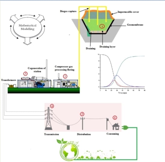
5.6. Potential for Energy Recovery by Cogeneration

The cogeneration unit consists of a gas engine or turbine, an alternator and optional heat recovery circuits. The gas is burned in the engine and then the mechanical energy of the engine is transformed into electricity via the alternator (Figure 8).

Well before cogeneration, the biogas purification step is necessary. This requires the presence of hydrogen sulphide at levels exceeding 900 ppm, which is the case for the controlled landfill in Fez, where the H₂S content in the biogas is around 1200 ppm compared with 600 ppm for the Mohammedia landfill (

Table 6. Biogas energy balance.

Year	MCH4 m3/Year	Total Energy GWh	Recoverable Energy GWh	Energy MWh
2012	5.91	58.81	55.87	6.38
2013	8.12	80.72	76.68	8.75
2014	1.60	15.82	15.03	1.77
2015	9.34	92.90	88.25	10.07
2016	8.16	81.13	77.08	8.79
2017	8.69	86.37	82.05	9.37
2018	9.16	91.09	86.54	9.88
2019	5.17	51.35	48.78	5.57
2020	5.19	51.51	48.94	5.59
2021	5.20	51.68	49.10	5.60
2022	5.22	51.85	49.26	5.62
2023	5.23	52.02	49.42	5.64
2024	5.25	52.19	49.58	5.66
2025	5.28	52.36	49.74	5.68
2026	5.28	52.53	49.90	5.70
2027	5.30	52.70	50.07	5.71
2028	5.30	52.70	50.07	5.71
2029	5.34	53.04	50.39	5.75
2030	5.35	53.21	50.56	5.771
2031	5.37	53.39	50.72	5.79
2032	5.39	53.56	50.88	5.80
totaux	124.85	1240.99	1178.94	134.58

).

The total annual energy produced from biogas is the product of the volume of methane multiplied by its lower calorific value, which is 9.94 kWh/m³ under normal temperature and pressure conditions [21,22,23,24,25,26,27,28].

$$E_{totale}=PC{I}_{CH\mathbf{4}}\times V_{CH\mathbf{4}} \left[KWh\right]$$

(12)

We allow for 5% energy loss in order to be sure that the engine is more supercharged than underfuelled [22]. The energy recoverable by the motor is therefore as follows:

$$E_{Valorisable}=\mathbf{0.95}\times E_{totale} \left[KWh\right]$$

(13)

$$E_{t=\mathbf{1}h}=\frac{E_{Valorisable}}{\mathbf{365}\times \mathbf{24}} \left[KW\right]$$

(14)

Taking into account an Et = 1 h average of 7288 KW, the gas engine would need to be designed to operate between 50% and 100% of its rated load, with an optimal efficiency around 75%. We are therefore looking for an engine with a power of about 9715 kW to be close to this optimum [12,21,22,23,24,25,26,27,28].

6. Conclusions

The projected depletion of fossil energy resources associated with the environmental issue of global warming has intensified the interest in renewable energies and the possible options they can offer. In this research study, it was possible to determine the value of the methanogenic potential of household waste and other substrates of the landfill of the city Mohammedia, which were significantly higher than the values usually used in modelling efforts due to the high proportion of organic waste. From an analysis of the total stability of the mathematical model of the process equilibrium, we constructed a criterion that, based on the inputs of the process and the parameters of the model, determines whether the mode of operation represents a risk to the sustainability of the process. The volume of methane that would be generated after twenty years of operation is of the order of 124,848,407 m³, thus producing 1,178,943,512 KWh of recoverable energy, a very large deposit that justifies investment.

References

- Bouhadiba, B.; Mezouri, F.; Kehila, Y.; Matejka, G. For an integrated Management for Municipal solid wast in Algeria.Systemic and Methodological Approaches. Int. Rev. Chem. Eng. Rapid Commun. 2010, 2, 426–429. [Google Scholar]
- Gu, Y.; Zhou, G.; Wu, Y.; Xu, M.; Chang, T.; Gong, Y.; Zuo, T. Environmental performance analysis on resource multiple-life-cycle recycling system: Evidence from waste pet bottles in China. Resour. Conserv. Recycl. 2020, 158, 104821. [Google Scholar] [CrossRef]
- Gautam, P.; Kumar, S.; Lokhandwala, S. Energy-aware intelligence in megacities. In Current Developments in Biotechnology and Bioengineering; Elsevier: Amsterdam, The Netherlands, 2019; pp. 211–238. [Google Scholar]
- Joseph, O.; Rouez, M.; Métivier-Pignon, H.; Bayard, R.; Emmanuel, E.; Gourdon, R. Adsorption of heavy metals on to sugar cane bagasse: Improvement of adsorption capacities due to anaerobic degradation of the biosorbent. Environ. Technol. 2009, 30, 1371–1379. [Google Scholar] [CrossRef] [PubMed]
- Mabrouki, J.; Moufti, A.; Bencheikh, I.; Azoulay, K.; El Hamdouni, Y.; El Hajjaji, S. Optimization of the Coagulant Flocculation Process for Treatment of Leachate of the Controlled Discharge of the City Mohammedia (Morocco). In Proceedings of the International Conference on Advanced Intelligent Systems for Sustainable Development, Tangier, Morocco, 8–11 July 2019; Springer: Cham, Switzerland, 200; pp. 200–212. [Google Scholar]
- Finon, D. La pénétration à grande échelle des ENR dans les marchés électriques. La perte de repère des évaluations économiques. Rev. De L’energie 2016, 633, 366–390. (In French) [Google Scholar]
- Mabrouki, J.; Moufti, A.; Bencheikh, I.; Azoulay, K.; El Hamdouni, Y.; El Hajjaji, S. Optimization of the Coagulant Flocculation Process for Treatment of Leachate of the Controlled Discharge of the City Mohammedia (Morocco). In Advances in Intelligent Systems and Computing, Proceedings of the International Conference on Advanced Intelligent Systems for Sustainable Development (AI2SD-2018), Tangier, Morocco, 12–14 July 2018; Ezziyyani, M., Ed.; Springer: Berlin/Heidelberg, Germany, 2018; pp. 200–212. [Google Scholar]
- Andriani, D.; Atmaja, T.D. The potentials of landfill gas production: A review on municipal solid waste management in Indonesia. J. Mater. Cycles Waste Manag. 2019, 21, 1572–1586. [Google Scholar] [CrossRef]
- Mabrouki, J.; El Yadini, A.; Bencheikh, I.; Azoulay, K.; Moufti, A.; El Hajjaji, S. Hydrogeological and hydrochemical study of underground waters of the tablecloth in the vicinity of the controlled city dump Mohammedia (Morocco). In Advances in Intelligent Systems and Computing, Proceedings of the International Conference on Advanced Intelligent Systems for Sustainable Development (AI2SD-2018), Tangier, Morocco, 12–14 July 2018; Ezziyyani, M., Ed.; Springer: Berlin/Heidelberg, Germany, 2018; pp. 22–33. [Google Scholar]
- El Maguiri, A.; Fawaz, N.; Abouri, M.; Idrissi, L.; Taleb, A.; Souabi, S.; Vincent, R. Caractérisation physique et valorisation des déchets ménagers produits par la ville de Mohammedia, Maroc. Rev. Nat. Technol. C. Sci. L’environ. 2016, 14, 16–25. [Google Scholar]
- Elkadi, A.; Maatouk, M.; Raissouni, M.; Chafik, T.; Mouhssine, A. Caractérisation des déchets ménagers et assimilés de la ville de Tanger/Characterization of household and assimilated waste in the city of Tangier. Int. J. Innov. Appl. Stud. 2016, 18, 512. [Google Scholar]
- Mabrouki, J.; Bencheikh, I.; Azoulay, K.; Es-soufy, M.; el Hajjaji, S. Smart Monitoring System for the Long-Term Control of Aerobic Leachate Treatment: Dumping Case Mohammedia (Morocco). In Big Data and Networks Technologies, Proceedings of the 3rd International Conference on Big Data and Networks Technologies (BDNT 2019), Leuven, Belgium, 29 April–2 May 2019; Springer: Berlin/Heidelberg, Germany, 2019; pp. 220–230. [Google Scholar]
- El Asri, O.; Afilal, M.E.; Laiche, H.; Elfarh, A. Evaluation of physicochemical, microbiological, and energetic characteristics of four agricultural wastes for use in the production of green energy in Moroccan farms. Chem. Biol. Technol. Agric. 2020, 7, 1–11. [Google Scholar]
- Mabrouki, J.; Benbouzid, M.; Dhiba, D.; El Hajjaji, S. Simulation of wastewater treatment processes with Bioreactor Membrane Reactor (MBR) treatment versus conventional the adsorbent layer-based filtration system (LAFS). Int. J. Environ. Anal. Chem. 2020, 1–11. [Google Scholar] [CrossRef]
- Porowska, D. Review of Research Methods for Assessing the Activity of a Municipal Landfill Based on the Landfill Gas Analysis. Period. Polytech. Chem. Eng. 2021, 65, 167–176. [Google Scholar] [CrossRef]
- Mabrouki, J.; Fattah, G.; Al-Jadabi, N.; Abrouki, Y.; Dhiba, D.; Azrour, M.; Hajjaji, S.E. Study, simulation and modulation of solar thermal domestic hot water production systems. Model. Earth Syst. Environ. 2022, 8, 2853–2862. [Google Scholar] [CrossRef]
- Ortiz-Oliveros, H.B.; Flores-Espinosa, R.M. Design of a mobile dissolved air flotation system with high rate for the treatment of liquid radioactive waste. Process. Saf. Environ. Prot. 2020, 144, 23–31. [Google Scholar] [CrossRef]
- Spokas, K.; Bogner, J.; Chanton, J.P.; Morcet, M.; Aran, C.; Graff, C.; Hebe, I. Methane mass balance at three landfill sites: What is the efficiency of capture by gas collection systems? Waste Manag. 2006, 26, 516–525. [Google Scholar] [CrossRef] [PubMed]
- Hijazi, O.; Munro, S.; Zerhusen, B.; Effenberger, M. Review of life cycle assessment for biogas production in Europe. Renew. Sustain. Energy Rev. 2016, 54, 1291–1300. [Google Scholar] [CrossRef]
- Scharff, H.; Jacobs, J. Applying guidance for methane emission estimation for landfills. Waste Manag. 2006, 26, 417–429. [Google Scholar] [CrossRef]
- Mouhssine, A.; Brigui, J. Organic waste characterization in Tangier City and evaluation of its potential biogas. Int. J. Innov. Appl. Stud. 2017, 20, 1042–1052. [Google Scholar]
- Mabrouki, J.; Azrour, M.; Hajjaji, S.E. Use of internet of things for monitoring and evaluating water’s quality: A comparative study. Int. J. Cloud Comput. 2021, 10, 633–644. [Google Scholar] [CrossRef]
- El Baz, F.; Arjdal, S.; Bakrim, M.; Mediouni, T.; Faska, N. Methanisation of Agadir urban solid waste: Theoretical evaluation of the energy production potential. In Materials Today, Proceedings of the International Congress: Applied Materials for the Environment (CIMAE-2018), Agadir, Morocco, 5–7 December 2018; Dahham, O.S., Zulkepli, N.N., Eds.; Elsevier: Amsterdam, The Netherlands, 2019; pp. 97–99. [Google Scholar]
- Wu, Z.L.; Lin, Z.; Sun, Z.Y.; Gou, M.; Xia, Z.Y.; Tang, Y.Q. A comparative study of mesophilic and thermophilic anaerobic digestion of municipal sludge with high-solids content: Reactor performance and microbial community. Bioresour. Technol. 2020, 302, 122851. [Google Scholar] [CrossRef]
- Trianni, A.; Cagno, E.; Accordini, D. Energy efficiency measures in electric motors systems: A novel classification highlighting specific implications in their adoption. Appl. Energy 2019, 252, 113481. [Google Scholar] [CrossRef]
- Blewitt, J. Deschooling society? A lifelong learning network for sustainable communities, urban regeneration and environmental technologies. Sustainability 2010, 2, 3465–3478. [Google Scholar] [CrossRef] [Green Version]
- Suther, T.; Fung, A.; Koksal, M.; Zabihian, F. Macro level modeling of a tubular solid oxide fuel cell. Sustainability 2010, 2, 3549–3560. [Google Scholar] [CrossRef] [Green Version]
- Richardson, R.B. Ecosystem services and food security: Economic perspectives on environmental sustainability. Sustainability 2010, 2, 3520–3548. [Google Scholar] [CrossRef]
Figure 1.
Device for measuring methanogenic potential by the displacement of water [9].
Figure 2.
Tonnage of green waste, poultry droppings and tannery waste.
Figure 3.
Annual tonnage of household waste.
Figure 4.
Average of the mass percentages of the fractions from the household and similar waste in the city of Mohammedia.
Figure 5.
Biogas production kinetics for the four types of waste in ml.
Figure 6.
Modeling results of CH4 production via the four models.
Figure 7.
(A) % tonnage; (B) % contribution to CH4 production of the four substrates.
Figure 8.
Overview of the cogeneration station [20].