
Modelling the Returnable Transport Items (RTI) Short-Term Planning Problem

Université Paris-Saclay, CentraleSupélec, Laboratoire Génie Industriel, 3 rue Joliot-Curie, 91190 Gif-sur-Yvette, France
*
Author to whom correspondence should be addressed.
Sustainability 2022, 14(24), 16796; https://doi.org/10.3390/su142416796
Submission received: 10 November 2022
/
Revised: 4 December 2022
/
Accepted: 12 December 2022
/
Published: 14 December 2022
(This article belongs to the Special Issue Managing Sustainable Development: Technology, Modelling & Applications)
Abstract
:Returnable transport items (RTI) are used for the handling and transportation of products in the supply chain. Examples of RTIs include plastic polyboxes, stillages or pallets. We consider a network where RTIs are used by multiple suppliers to deliver parts packed in RTIs to multiple customers. We address the short-term planning of empty-RTI flows (i.e., reverse flows) which consists of optimizing the transportation routes used to return empty RTIs from customers to suppliers. A transportation route consists of one or several trucks traveling from a customer to a supplier at a given frequency. The RTI short-term planning problem is critical because it impacts the continuity of loaded-RTI flows and affects the transportation and shortage costs of empty RTIs incurred at the very-short-term. We study a heterogeneous fleet of automotive parts RTIs, under two configurations: pool RTIs, which are standard RTIs shared between suppliers, and dedicated RTIs that are specific to each supplier. To solve the short-term planning problem, we develop a two-step approach using mixed-integer linear programming (MILP) and a greedy heuristic. For pool RTIs, our models enable a reduction of 30% in the number of trucks used and 20% in the distance traveled. Furthermore, if dedicated and pool RTIs are jointly planned, this would enable a 9% gain in terms of transportation costs.
1. Introduction
Over the past 10–15 years, against a background of increasing public and government concern for environmental issues, companies have come under mounting pressure to improve the environmental impact of their logistics operations. In particular, as stated in [1], the transport industry produces 25% of global CO2 emissions; looking at the future of the transport sector, this will increase over the coming decades. There are ways to focus on being green and the reduction of CO2 without swapping the entire company fleet. Transport optimization is one such lever that has a direct impact on CO2 emissions. In this paper, we are interested in reverse logistics, particularly in the transport optimization of the reverse flow of returnable packaging called Returnable Transport Items (RTI). Examples of RTIs include pallets, containers, reusable boxes, stillages, etc. Indeed, RTIs are increasingly used in several industries both for economic and environmental factors. In terms of environmental impacts, compared to disposable (i.e., single-use) packaging, RTIs are known to reduce the use of raw materials and decrease waste production. From an economic perspective, the use of RTIs can reduce purchase and disposal costs.
For those RTIs, the forward flows consist of suppliers delivering parts packed in RTIs to customers (i.e., loaded RTIs). Reverse flows consist of customers returning empty RTIs to suppliers. The reverse flows of empty RTIs raise various planning issues from a supply chain perspective, as presented in Figure 1. First, we distinguish long-term planning (3–5 years) related to empty-RTI network design. It involves issues such as defining the empty-RTI return logistics structure and the level of integration with forward flows. Secondly, there is mid-term planning (6–12 months) of sizing the RTI fleet, which consists in optimizing the number of RTIs to acquire to minimize overall costs. Then, in short-term planning (4–8 weeks), the main objective is to set the transportation framework within which the daily operations of empty-RTI flows will be performed. Finally, at the very-short-term level (1–7 days), a distribution plan optimizes the daily quantity of empty RTIs to be returned to suppliers.
This paper is devoted to the short-term planning issue, i.e., the optimization of the transportation routes needed for the distribution of empty RTIs. The objective is to set the transportation framework within which the daily operations of empty-RTI flows will be performed. Indeed, the definition of transportation routes in the short-term consists of planning a set of trucks to transport empty RTIs from customers to suppliers to enable the distribution of empty RTIs at the very short-term level. Then, at the very-short-term level, a distribution plan is designed to optimize the daily quantity of empty RTIs to be returned to suppliers: the objective is to determine, for each type of RTI, which customers return empty RTIs to which suppliers and in what quantity. The optimization of the transportation routes at the short-term level is critical since it has an impact on transportation and shortage costs incurred in the very-short-term planning.
The main issue in the RTI short-term planning problem is to determine the optimal transportation flows and frequencies that minimize transportation costs under the constraint of a fixed RTI fleet size. The routes (i.e., set of trucks traveling from a customer to a supplier at a given frequency) must be optimized in such a way as to reduce distances, increase truck fillings and therefore minimize transportation costs. Moreover, they must be consistent with the customers’ release and the suppliers’ demand volumes. On the other hand, return frequencies (i.e., number of returns per period) must be determined in such a way as to minimize transportation cost while taking into account the RTI fleet constraint. Indeed, as demonstrated by [2,3], a high delivery frequency would generate high transportation cost and probably lead to cancelled routes at the very-short-term level. Conversely, a low return frequency may generate shortage cost if the supplier does not have sufficient empty-RTI inventory to cover its demand until the next delivery, or increased transportation cost if additional spot transportation orders are requested in the very-short-term planning level.
This paper is based on an industrial case in the automotive sector where the very-short-term RTI planning is based on transportation routes that are defined earlier. The transportation routes are pre-contracted with the carriers and performed on a fixed and regular basis over a period of time. Then, in the very-short-term planning, the transportation routes are used to plan the daily distribution of empty RTIs. This involves defining the quantity of empty RTIs to be returned on each customer–supplier link via transportation route trucks that are already defined at short-term planning and, if necessary, through spot trucks to adapt to minor flow fluctuations. Actually, the company will encounter some problems in optimizing the short-term planning of empty RTIs, which generates over costs of transportation and shortages at the very-short-term. Indeed, experts rely on historical data to define the transportation routes. Consequently, the transportation routes are not optimized regularly and are changed only when the transportation performance deteriorates significantly at the very-short-term level. Furthermore, the transportation routes are defined manually. Hence, they are not regularly updated because of the complexity of the flows, the multiplicity of suppliers and customers, and the diversity of RTIs. Indeed, the change of transportation routes from a given customer to a given supplier can impact the transportation routes of other customers and suppliers.
The company’s interests for the very-short-term planning based on transportation routes are multiple. Firstly, it provides a large part of the transportation capacity needed to carry out empty-RTI flows at the very-short-term level. On the other hand, it allows them to foresee the planning of shipping and receiving operations at the level of customers and suppliers. Secondly, it avoids having to redefine a transportation plan on a daily basis, as a majority of the flows travel on transportation routes. Finally, it allows negotiating more competitive transportation costs. Indeed, transportation routes allow carriers to plan the necessary resources and optimize them to execute the transportation routes, which results in lower costs.
In addition, two types of RTI flow management are used in the network studied: pool mode and dedicated mode. In pool mode, RTIs are used indifferently by different suppliers to deliver parts to different customers (i.e., RTIs are not specific to a part, a supplier or a customer); the customer which returns empty RTIs to each supplier is not necessarily the one who received the same RTIs that were loaded with parts. The dedicated mode is simpler to manage because RTIs circulate in a closed loop between the same supplier and customer. The pool mode is more efficient in reducing the return distances, and the number of RTIs needed in the network. In particular, when the dedicated mode is used, each supplier holds its inventory of RTIs, while empty RTIs are easily lost or misplaced in pool mode. Currently, short-term planning for dedicated and for pool RTIs are done separately in the company. The lack of a decision support model prevents their joint optimization.
The contribution of this paper is to propose an approach for defining the transportation routes; the developed models optimize the transportation costs under the constraint of a fixed RTI fleet size. We solve these models for a multi-supplier, multi-customer and multi-RTI supply chain. This issue has not been widely studied in the literature, and in particular for large complex networks, as is the case in the automotive sector. The remainder of this paper is organized as follows: Section 2 presents a literature review on research related to our problem. In Section 3, we present the principles of the model and the approach we propose. Section 4 is dedicated to the detailed mathematical formulations of the problem. Finally, a case study is conducted to illustrate the applicability of the approach in the company studied.
2. Literature Review
RTI supply chains often involve multiple stakeholders, from RTI manufacturers to RTI users, including other levels such as RTI pooling providers, RTI cleaning and repair providers, RTI recyclers, etc. The different stakeholders must deal with a myriad of complex decisions to manage RTI supply chains. A summary of these decisions in the context of RTIs is presented in [4] with a particular focus on the different stakeholders involved in the RTI supply chain and their economic and environmental performance. Three decision levels are identified: strategy and design of the RTI system, management of RTI logistics and management of RTI operations (production, repair, end of life).
The implementation of an RTI supply chain requires the management of information systems to track the flows in an efficient way. The use of RFID technologies leads to improved information on the return of empty RTIs, as suggested by [5] who proposed a method for managing and evaluating the use of RFID in the tracking of reusable containers. From a technical point of view, ref. [6] developed a framework for the architecture and design of the information technologies for the pooling service of an innovative RTI in the grocery supply chain.
Other researchers have addressed specific issues related to RTI operations management. Ref. [7] studied empty-RTI network design in the food industry. They developed a mixed-integer linear programming model dealing with facilities opening and allocating empty-RTI flows across the network. In addition to network design, a critical decision in RTI supply chain consists of sizing the RTI fleet. Ref. [8] proposed a model the find the optimal number of RTIs to invest in to minimize the total operating cost in the automotive industry under stochastic demand and lead-time.
A few other papers have focused on problems related to RTI inventory management. Ref. [9] proposed a model to determine the optimal RTI purchasing cycle and inspection length to minimize total expected inventory costs in the case of a single supplier, single retailer and single RTI type. Ref. [10] proposed an inventory model considering RTI loss to ensure the continuity of the forward flows of RTIs loaded with products. The objective is to define the number of replenishments of new RTIs, the quantity of empty RTIs returned per cycle and the loss rate of RTIs to minimize the inspection and ordering costs of RTIs.
Several authors have performed studies on RTI transportation planning, particularly on the RTI inventory routing problem. Ref. [11] developed a multi-period inventory routing model with pick-up and delivery to minimize the total cost, including inventory holding, screening, maintenance, transportation, sharing and purchasing costs for new RTIs. Ref. [12] addressed a similar issue with an application to perishable food, considering RTIs with different food quality preservation abilities, and the simultaneous delivery of food and pick-up of RTIs. Ref. [13] proposed a cluster-first route-second mat-heuristic to solve the inventory routing problem under time windows constraints in the context of a single supplier, multiple customers and a single RTI type. Finally, ref. [14] suggested to integrate demand uncertainty using a probabilistic mixed-integer linear programming model that minimizes holding costs, transportation costs with explicit fuel consumption, demand uncertainty and multiple products.
Sustainability aspects have also been addressed by different authors in relation to RTI management decision problems. Efforts towards the achievement of sustainable logistics require the extension of traditional economic supply chain objectives (such as reduced costs and improved delivery reliability) to include environmental objectives. In the specific area of transport and logistics services, this means that actors must pay more attention to transport and logistics operations that go beyond the traditional trade-off between cost and customer service. In the context of RTI supply chain, ref. [15] dealt with RTI network design decisions while integrating a green aspect to minimize carbon emissions in addition to the maximization of supply chain profit. Similarly, ref. [16] studied the environmental and economic impacts of RTI flows under different network and pooling configurations in the retail supply chain. Ref. [17] investigated the issue of minimizing environmental emissions in an RTI supply chain. They developed a simulation model coupled with an optimization model to find the optimal setting that minimizes the environmental emissions of RTI flows.
The work that most closely relates to our research is that of [2]. The author addresses flows and frequencies decisions, under a fixed RTI-fleet-size constraint, in a large network made up of several suppliers and customers with a single RTI type. He proposes a model to allocate the flows between customers and suppliers and to define the optimal delivery batches that optimize transportation cost. The approach is characterized by constant demand and release rates and continuous return frequencies. The author distinguishes two cases depending on transportation capacity. The author then proposes two extensions of the fundamental model to integrate distribution centers into the network and to model a greater diversity of RTIs. This last extension could only be solved in the case of a single customer and multiple suppliers.
The work of [2] makes an important contribution. However, it does not allow dealing with several types of RTIs as is the case in our context. If a customer returns several types of empty RTIs to a supplier, they are transported in the same truck to share the transportation cost. Therefore, the optimization of flows and frequencies must be done simultaneously considering the different types of RTIs, which adds further complexity to the problem.
The main contribution of this paper is to propose a comprehensive approach to defining empty-RTI flows and frequencies while integrating a strong transportation perspective when optimizing flows. Thus far in the literature, as summarized in Table 1, empty-RTI flows and frequencies decisions have been considered separately without establishing a link between them. The connection between these two decisions is an important issue to ensure consistency between transportations decisions and empty-RTI flow and fleet size constraints. We develop two models that define a set of transportation routes optimizing transportation cost while adapting to flow constraints (supplier demands and customer releases) and RTI fleet size. Models are applied to large networks including several types of RTIs, multiple customers and multiple suppliers. We therefore deal with the more general and complex case of pool RTIs, compared to the single-customer, single -supplier and single-RTI models which are more relevant to the simpler case of dedicated RTIs.
3. Problem Modelling and Proposed Approach
The objective of this section is to describe in more detail the empty-RTI short-term planning problem and the proposed approach to address it.
3.1. Modelling Assumptions
We consider a logistics network made up of a set of suppliers and a set of customers with a heterogeneous fleet of RTIs that circulate in a closed loop (c.f. Figure 2).
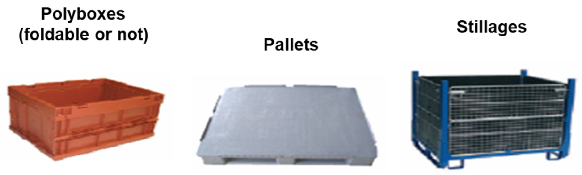
We are interested in different types of empty RTIs circulating between customers and suppliers. RTIs vary in function with different parameters such as size, weight and materials. The RTI types studied consist of polyboxes and stillages of different sizes, which can be collapsible (foldable) and non-collapsible. These RTIs are transported in standard semi-trailer trucks.
Two types of empty-RTI flow management are used in the network (see Figure 3). In the pool mode, the decision of which customer returns an empty RTI to which supplier is not known in advance; it must be determined in such a way as to minimize transportation cost. In the dedicated mode, RTIs are used by a specific supplier to deliver parts to a specific customer. In this case, the reverse flow is predefined: the customer who receives the loaded RTI is the one who returns the empty RTI to the supplier.
In the context of the automotive manufacturer studied, the return flow of pool RTIs is managed by a central unit of the automaker that contracts with carriers to return the empty RTIs. This is because pool RTIs are standardized and owned by the automaker itself and not the suppliers.
Each customer holds an inventory of loaded RTIs, received from one or several suppliers (see Figure 4). It consumes the parts inside the RTIs and releases empty RTIs at a release rate, depending on the characteristics of its production process. Empty RTIs are transported in batches to the suppliers to optimize transportation cost, which generates an inventory of empty RTIs at suppliers.
Similar to customers, each supplier holds an inventory of empty RTIs (see Figure 4), received from one or several customers. It consumes empty RTIs to pack its parts at a demand rate, depending on the characteristics of its production process. Transportation of loaded RTIs is also peformed by batch to optimize transportation cost, which creates an inventory of loaded RTIs at customers.
Suppliers and customers consume and release empty RTIs at a constant rate. Hence, average values are used for suppliers’ demand and customers’ release. In addition, the average demand and release rates of empty RTIs are considered to be completely balanced between the set of suppliers and the set of customers. Data analysis from the industrial case study confirming this hypothesis is presented in Appendix A.
The transportation of empty RTIs takes a lead time that mainly depends on the distance between the customer and the supplier (see Figure 4).
The RTI fleet size for each RTI type is fixed. Indeed, the fleet size is defined (i.e., optimized) at the mid-term level. That is why, in the short-term models developed in the current paper, we assume that the RTI fleet size for each RTI type is fixed, and this size cannot be varied.
The return frequency (i.e., the number of trucks) on a given customer–supplier link must respect a minimum return frequency. This is a constraint related to the information systems that manage the transportation routes at the studied company. It expresses the fact that each transportation route must have at least one truck planned per week.
3.2. RTI Inventory Requirement and Fleet Size
The optimization of empty-RTI transportation routes is done by taking into account the effect of this optimization on the quantity of RTI inventory needed in the network. As shown in Figure 4, RTIs circulate in a closed loop. In the forward flows, suppliers deliver parts packed in RTIs to customers (i.e., loaded RTIs). In the reverse flows, the customers return empty RTIs to the suppliers.
In a closed-loop supply chain, RTI inventory is needed at multiple stages of the network for various reasons.
First, suppliers would keep an inventory of empty RTIs if they manufacture parts in batches, to amortize fixed production cost, or if they hold a safety inventory to compensate for the uncertainty of empty-RTI returns. Then, RTIs can be used to store and handle semi-finished parts during the intermediate phases of production. At a later stage, finished parts are stored until they are delivered to customers; if parts are delivered in batches, an inventory of loaded RTIs is built up.
Similar to suppliers, customers can hold an inventory of loaded RTIs upstream of their production process. An inventory of parts may be necessary against transportation lead time or demand variability in the forward flows, or to compensate for the calendar gap between production and transportation processes or between customers’ and suppliers’ production rates. As parts are used in customers’ manufacturing processes, RTIs are needed to ensure their handling and storage along the production process. Finally, an inventory of empty RTIs will be built up if RTIs are returned to suppliers in batches.
There is also an in-transit inventory during transportation operations for both loaded and empty RTIs.
3.3. RTI Short-Term Planning Approach
The objective of the short-term planning is to optimize the transportation routes, which consist of one or several trucks traveling from a customer to a supplier at a given return frequency. Indeed, the short-term planning consists of two decisions: defining the quantities that will be transported on each customer–supplier link for each RTI type and defining the return frequency for each link. The first challenge is to minimize transportation cost by returning empty RTIs to suppliers from the closest customers with a minimum number of trucks. Low return frequencies allow an increase in the size of the delivery batches and thus optimize the filling of the trucks. However, they imply the need for a large number of RTIs necessary to constitute larger delivery batches. Since the RTI fleet size for each RTI type is fixed in the short-term level, the objective of the short-term planning is to optimize the transportation cost while respecting the RTI fleet-size constraint.
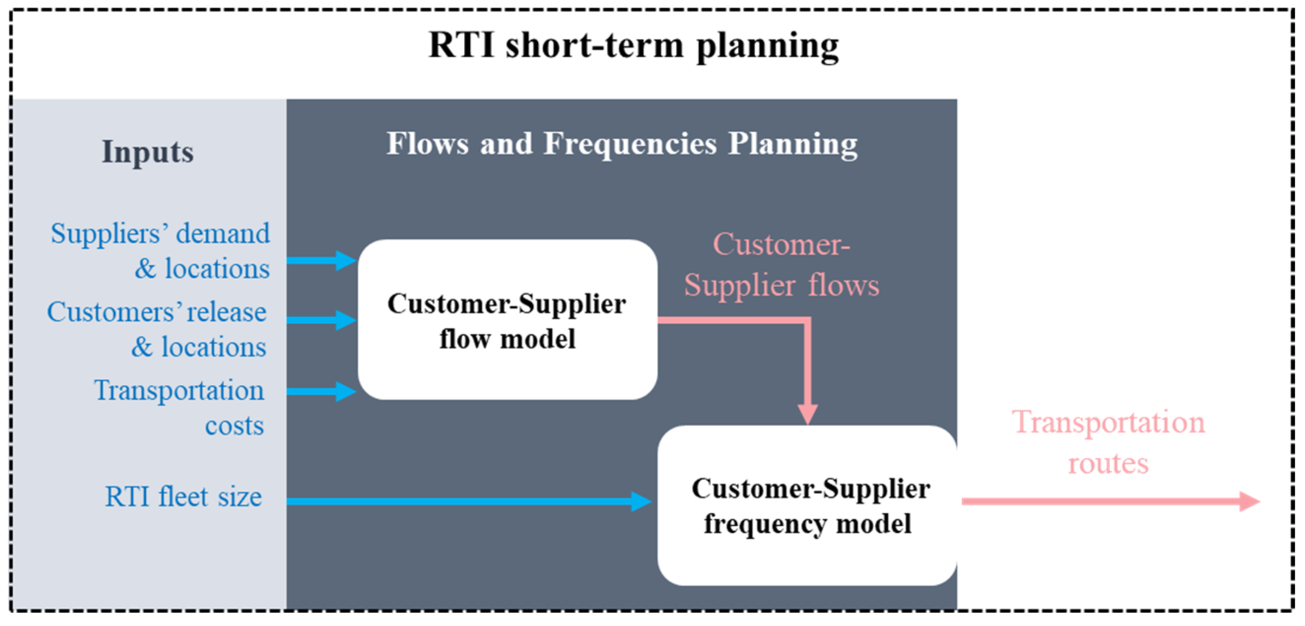
As illustrated in Figure 5, our approach consists of first determining the flows with an assumption of a large RTI fleet size, and then optimizing the return frequencies under the constraint of the RTI fleet size:
- Customer–Supplier Flow model: This first step is to define which customers return empty RTIs to which suppliers, with which quantity, and the optimal return frequency over each customer–supplier link. The optimal return frequency represents the minimum number of trucks to return empty RTIs with optimized transportation cost. In this model, the RTI fleet-size limit is not taken into consideration (the RTI fleet size is assumed very large), and only transportation cost is optimized with the assumption of a very large fleet size. The objective is to return enough empty RTIs to cover the demand of the suppliers using the available release at customers while minimizing the transportation cost. Additionally, we integrate a minimum return frequency per customer–supplier relative to the company studied. At the end of this step, we obtain optimal flow allocation decisions (which customer return empty RTIs to which supplier) and the optimal return frequency per customer–supplier link.
- Customer–Supplier Frequency model: This second step consists in introducing the RTI fleet-size constraint and to eventually reduce delivery batches so that, for each type of RTI, the variable empty-RTI inventory requirement is covered by the available quantity of RTIs. This is done by increasing the return frequency on selected customer–supplier links in order to minimize additional transportation cost. This means that flow allocation decisions (i.e., which customer return empty RTIs to which supplier) are fixed in the previous step, and that only return frequencies will be re-optimized. This is because the optimization of flows from a transportation point of view also indirectly optimizes the use of empty RTI inventory through a reduction of delivery distances. At the end of this step, we obtain, for each customer–supplier link, the return frequency that allows to respect the RTI fleet-size constraint.
Figure 5.
The proposed approach for RTI short-term planning.
3.4. Model Formulation
The objective of this section is to present the detailed mathematical formulation of models used in the proposed approach for empty-RTI short-term planning. We first present the overall RTI inventory requirement formulation that is used in the RTI fleet-size constraint. Then, we present the Customer–Supplier Flow and Customer–Supplier Frequency models used to optimize empty-RTI flows and frequencies between customers and suppliers under RTI fleet-size constraint. The Customer–Supplier Flow model is formulated as an MILP. Subsequently, the Customer–Supplier Frequency model is solved using a greedy heuristic. The sequential approach of first determining the flows with an assumption of a large RTI fleet size and then optimizing the return frequencies under the constraint of the RTI fleet size was adopted to avoid nonlinear models that would be difficult to solve in our industrial context. The overall model pattern is described in Figure 6.
3.4.1. Notations
Sets
- K: the set of suppliers.
- J: the set of customers.
- R: the set of RTI types.
Parameters
- : the average internal transit time for an empty RTI at supplier , which includes the storage time from the arrival of the empty RTI and the processing time along the production line of the supplier until the empty RTI is loaded with parts.
- : the average transportation lead time for a loaded RTI between supplier to customer (forward flows).
- : the average internal transit time for a loaded RTI at the customer , which includes the storage time from the arrival of the loaded RTI and the processing time along the production line of the customer until the loaded RTI is emptied of parts.
- : the average transportation lead time for an empty RTI between supplier to customer (reverse flows).
- : the average periodic flow of a loaded RTI of type , delivered by supplier to customer (forward flows).
- : the average delivery batch for loaded RTIs delivered from the supplier to the customer for the RTI of type (forward flows). For example, could be 1000 loaded RTI units per week and could be 500 units, meaning that two deliveries are performed per week with a quantity of 500 units per delivery to satisfy the 1000 loaded RTI units.
- : the average periodic quantity of empty RTIs of type demanded by supplier .
- : the average periodic quantity of empty RTIs of type released by the customer .
- : the transportation cost charged for a truck returning empty RTIs from customer to supplier .
- : the maximum quantity of empty RTIs of type that can be transported in a truck. It should be noted that the capacity of trucks for loaded and empty RTIs can be different if the RTIs are collapsible (foldable). In our study, we have both cases: collapsible and non-collapsible RTIs. In the parameter , we take this aspect into account by computing the number of empty RTIs that can be transported in a truck.
- : the minimum return frequency per customer–supplier link (in number of trucks per period).
- : time bucket parameter (in number of periods) (minimum period in which we will have at least one delivery).
- : the fixed inventory requirement for loaded RTIs of type to operate the forward flows (independent of the short-term planning problem, because our models study only the reverse flows of empty RTIs sent by customers to suppliers).
- : the total quantity of RTIs of type available in the network including loaded and empty RTIs (RTI fleet size).
- : the available quantity of empty RTIs of type in the network for the reverse flows.
- : the safety inventory of RTIs of type which compensates for the effects of variability that may be encountered at the very-short-term level. This parameter is set empirically (in our case, we compute it as a fraction of the total RTI inventory requirement), but it will be possible to check whether it is sufficient or not depending on the results of very-short-term planning. Typically, too many shortages would mean that the safety inventory must be increased.
- : the incremental value used to increase the return frequency at each iteration of the heuristic in the Customer–Supplier Frequency model.
Variables
- : the overall RTI inventory requirement for RTI type , i.e., the quantity of RTIs required for each type of RTI in the network considered, including loaded and empty RTIs.
- : the variable inventory requirement for empty RTIs of type to operate the reverse flows (dependent on the short-term planning problem).
- : the average periodic quantity of empty RTIs of type returned from customer to supplier (during time bucket T). This variable corresponds to the flow of empty RTIs on customer–supplier link optimized in the Customer–Supplier Flow model.
- : the average periodic return frequency between customer to supplier , which equals the average number of trucks used for each customer (during time bucket T). This variable corresponds to the return frequency of empty RTIs on customer–supplier link optimized in the Customer–Supplier Frequency model.
- : the average delivery batch for empty RTIs between customer to supplier for the RTIs of type . This variable corresponds to the flow of empty RTIs divided by the return frequency on customer–supplier link .
3.4.2. RTI Inventory Requirement Formulation
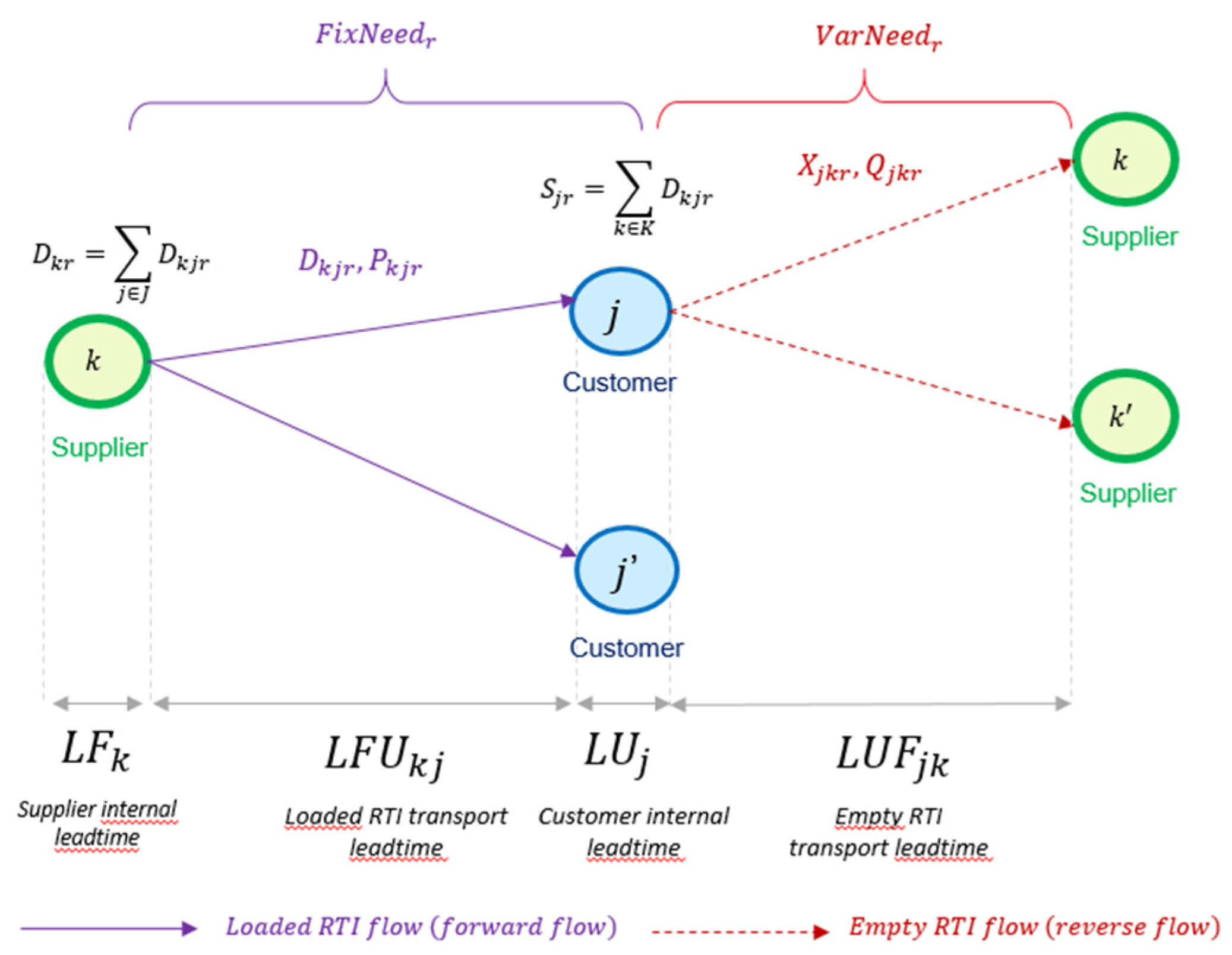
The formulation of the overall RTI inventory requirement depends on several parameters, as represented in detail in Figure 7. The flows of loaded and empty RTIs are considered to be balanced. However, the return frequency of empty RTIs may be different from the delivery frequency of loaded RTIs. In our study, we consider the delivery frequency of loaded RTIs to be fixed and seek to optimize the return frequency of empty RTIs. Since the delivery frequency of loaded RTIs is fixed, the inventory of RTIs required to operate the loaded RTI flows ( is pre-determined. With the remaining inventory of empty RTIs in the network (), we seek to define the return frequency of empty RTIs that minimize transportation costs while respecting the remaining inventory of RTIs (). In order to meet this constraint, we formulate the RTI inventory requirement ( to operate the flow of empty RTIs according to the parameters of our problem, which are the flows and the return frequencies of empty RTIs. This formulation allows us to check that the RTI inventory requirement for empty RTI flow is covered by the remaining inventory of RTIs.
We aim to formulate the overall RTI inventory requirement for each type of RTI in the network according to the system characteristics (suppliers’ demand, customers’ release, loaded- and empty-RTI transportation lead times, loaded- and empty-RTI flows, loaded- and empty-RTI return frequencies).
represents the necessary RTI inventory in the network of type to operate the loaded- and empty-RTI flows between suppliers and customers. The objective is to ensure that the RTI inventory requirement is covered by the actual available quantity of RTIs in the network.
is expressed as the sum of the fixed, the variable inventory requirement and a safety inventory:
We assume that the RTI fleet size in the system is predefined in the short-term models we develop. In order to avoid shortages, for each type of RTI, the RTI inventory requirement must be covered by the actual available quantity of RTIs in the network. This global satisfaction constraint of the RTI fleet size can be written as:
To formulate , we first concentrate on the calculation of , i.e., the variable inventory requirement for the RTIs of type to operate the reverse flows of empty RTIs. As represented in Figure 7, depends on two parameters and that are optimized in the Customer–Supplier Flow and Frequency models.
The variable RTI inventory requirement is given by:
The average empty-RTIs in-transit inventory represents the inventory of empty RTIs held in trucks during transport operations. On average, the quantity of empty RTIs is flowing on each (customer, supplier) link in each period. The average transport lead time is . According to Little’s Law, the average in-transit inventory is constant; it is equivalent to the average lead time spent by an empty RTI in the truck multiplied by the average flow over this period (i.e., the average quantity of empty RTIs returned by the customer to the supplier).
In the short-term planning problem, since we only make decisions about the reverse flows (hence the name “variable”), the fixed inventory requirement is given (i.e., it is a parameter of our models). A detailed formulation of the fixed inventory requirement is presented in Appendix A.
From the constraint:
And the equality:
We can deduce:
Or equivalently:
where the available quantity of empty RTIs of type in the network for the reverse flows is given by:
This constraint is used in the Customer–Supplier Frequency model to ensure that the RTI fleet-size constraint is respected.
As explained previously, our approach first optimizes flows and frequencies decisions from a transportation point of view by considering that the RTI fleet is very large (i.e., this is done in the Customer–Supplier Flow model which determines the flows and frequencies for each customer–supplier link). Then, the Customer–Supplier Frequency model re-optimizes the return frequencies under the constraint of the RTI fleet size, on a selected set of customer–supplier links taking into consideration the additional transportation cost.
3.4.3. Customer–Supplier Flow Model
The Customer–Supplier Flow model conceptually has two formulations. The first formulation uses continuous frequency variables with a full truck hypothesis. From an academic perspective, this is the one that reduces transportation costs the most. This means that return frequencies can be very low on customer–supplier links where volumes are low to ensure full truckload transportation. In the industrial context studied, we must consider two constraints. The first one is that the return frequencies must be integers to translate them into a number of trucks to build a transportation plan subsequently. The second is that the return frequencies must respect a minimum return frequency per customer–supplier link. For instance, a minimum return frequency of once a week means that at least one truck is scheduled per week on each customer–supplier link. Consequently, the Customer–Supplier Flow model is formulated as an MILP.
Objective Function
The objective function of the model is to minimize the average periodic transportation cost, over customer–supplier links, which is given by the sum of the number of trucks required multiplied by the transportation cost per truck on each link. It can be stated as follows:
Optimization Constraints
The first two constraints of the model are flow conservation constraints. The flow variables being defined as the quantity to be returned during the time bucket T, it must be equivalent to the demand/release per period multiplied by the time bucket T.
- The average total quantity of empty RTIs for each RTI type received by each supplier from all customers should be equal to its average demand:
- The average total quantity of empty RTIs for each RTI type returned by each customer to all suppliers should be equal to its average release:In the context studied, the return frequencies must respect a minimum return frequency per customer–supplier link. This constraint is related to the information systems that manage the transportation routes in the company studied. The frequency determined with the Customer–Supplier Flow and Frequency models on each customer–supplier link per period must be higher than the minimum return frequency set (e.g., a minimum return frequency of once a week means that at least one truck is scheduled per week on each customer–supplier link).
- The average frequency for each customer–supplier link is given by the average flow (i.e., quantity) over all types of RTIs divided by the maximum quantity that can be loaded in a truck. The return frequency during time bucket T can be seen as a round-up of the quantity transported during time bucket T divided by the truck capacity. Since the flow is calculated over the duration corresponding to the time bucket T, the return frequency will respect the minimum return frequency constraint because we consider only integer frequencies in the model.
- Finally, flow variables must be integer values. In addition, frequency values must also be integers so that we can translate them into a number of trucks to build the transportation routes subsequently.
3.4.4. Customer–Supplier Frequency Model
For the Customer–Supplier Frequency model, we propose a greedy heuristic which takes as an initial solution the results of the flow model, and then makes, at each iteration, a choice to increase the frequency on a cost-efficient flow to reduce the variable inventory requirement, while minimizing the additional transportation cost.
The purpose of the Customer–Supplier Frequency model is to increase the return frequencies on the most transportation cost-effective flows, which would reduce delivery batches and therefore the variable inventory requirement until the constraint of the RTI fleet size is met.
In the Customer–Supplier Frequency model, flow decisions remain the same as those obtained with the Customer–Supplier Flow model. Indeed, since the flow model minimizes transportation cost, it will naturally minimize the delivery distances and transportation lead times (i.e., ) and consequently the in-transit inventory in the trucks (i.e., ). Therefore, it is not interesting to change the flows in the Customer–Supplier Frequency model.
For the Customer–Supplier Frequency model, we propose a greedy heuristic which takes as initial solution the results of the flow model, and then makes, at each iteration, a choice to increase the frequency on a given flow in order to reduce the variable inventory requirement, while minimizing the additional transportation cost.
The main idea behind the proposed heuristic is to select at each iteration a flow between a customer and a supplier on which we will increase the frequency by one step. The choice of the flow will be based on two criteria:
- The increase in frequency must increase transportation cost as little as possible.
- The increase in frequency must reduce the variable inventory requirement for the RTI type in shortage as significantly as possible.
For a type of RTI, the shortage quantity is defined by the formula:
To model the first criterion, the derivative of transportation cost function with respect to frequency is used:
To model the second criterion, the derivative of the variable inventory requirement with respect to frequency is used:
To aggregate these two criteria, we introduce an overall criterion which takes the first criterion divided by the second criterion, weighted by the quantity of empty RTIs in shortage:
In order to choose the flows that minimize the first criterion and maximize the second, we should choose the flows that maximize the overall criterion.
This overall criterion obviously takes into account all types of RTIs combined. In fact, since the different types of RTIs are transported together, an increase in frequency for a given flow will impact the variable inventory requirement of all types of RTIs transported on the link.
The complete Customer–Supplier Frequency model is presented in Appendix A.
4. Case Study
The objective of this section is to apply our models to the industrial case studied. First, the company is interested in evaluating the use of the short-term planning models for the pool RTIs. Indeed, the definition of transportation routes does not follow a rigorous process within the company studied. The return frequencies implemented in transportation routes are mainly based on rules of thumb. These rules are mainly based on the volume of empty RTIs demanded by each supplier to determine its return frequency. This does not take into account the distance between suppliers and customers who return empty RTIs to them, the location of suppliers with respect to the others, and the types of empty RTIs requested, which may be in shortage or excess. As a result, the transportation costs of RTIs are high despite the relatively low service rate to suppliers. Since the definition of transportation routes is not based on a decision support tool, it is currently difficult for the company studied to obtain transportation routes that optimize transportation costs and consider the availability of empty RTIs in the network.
We run our model with a data set containing 1400 suppliers, 20 customers and 20 RTI types to obtain the best transportation routes with the greedy heuristic. Then, we compare transportation routes currently used in the company with those obtained with the short-term planning models (see Table 2).
Results show that the short-term planning models allow for a 30% reduction in the number of trucks used and a 20% reduction in the average distance travelled per truck.
Secondly, the company is interested in jointly optimizing the short-term planning of pool and dedicated RTIs. The objective is to evaluate the potential savings in terms of transportation cost and of empty-RTIs inventory requirement if we integrate the short-term planning of dedicated RTI flows with the one of pool flows. Indeed, dedicated and pool RTIs are currently managed independently. Hence, dedicated trucks similar to those considered so far circulate in the network to transport dedicated RTIs between the same suppliers and the same customers that use pool RTIs. In the industrial context studied, the flows of dedicated RTIs represent substantial volumes in the network and therefore have a significant impact on transportation costs. The objective would be to use the remaining transportation capacity in the trucks that already circulate in the network (trucks already planned in our models for pool RTIs) to transport dedicated RTIs. This would optimize transportation costs and reduce the variable RTI inventory requirement enabled by increased return frequency.
In the following, we use the short-term planning models developed to study the impact of mutualizing the short-term planning of dedicated RTIs with the pool RTIs studied so far.
The first question to be addressed is how to integrate dedicated-RTI flows into the flow and frequency planning models developed. Indeed, at the studied company, both pool and dedicated RTIs are transported in the network by the same transportation means indifferently. The flows that have been considered so far concerned empty RTIs managed in pool mode, as this is the most complex case to manage because the origin of empty-RTI flows, i.e., the customer who returns the empty RTIs to each supplier, is not known in advance and has to be optimized by a decision-making tool. On the contrary, for dedicated mode, each supplier–customer pair operates with its identified RTI flows. Therefore, the customer that returns empty RTIs to each supplier and the quantity of empty RTIs to be returned are predetermined. The only variable that remains to be determined is the return frequency. In the following, we propose to determine a global return frequency, i.e., for links where both pool RTIs and dedicated RTIs need to be transported, the frequency is based on the overall flow of both types of RTIs. To consider this issue, we use the Customer–Supplier Flow model to determine the pool RTI flows, as well as the overall frequencies that optimize transportation cost. Finally, we integrate RTI fleet-size constraints in the Customer–Supplier Frequency model to adjust the frequencies in such a way to match the variable RTI inventory requirements with the available quantity. The adaptation of short-term planning models developed for pool RTIs to integrate dedicated RTIs is detailed in Appendix A.
The results of the Customer–Supplier Flow model are presented in Table 3 for two scenarios: Scenario 0, where we apply the Flow and Frequency models separately for pool RTI flows on one side and for dedicated RTI flows on the other side (i.e., independently) and we sum up the costs obtained; and Scenario 1, where we apply the Flow and Frequency models to both pool and dedicated RTI flows and then calculate the associated costs.
The transportation cost obtained with the Customer–Supplier Flow model for Scenario 1 (joint planning of pool and dedicated RTI) is 8% lower than the one obtained for Scenario 0 (separate planning of pool and dedicated RTIs). This is due to the pooling of trucks to transport both pool and dedicated RTIs for suppliers who consume both types, which reduces transportation costs.
In the example we study, in order not to complicate the analysis of the results, we only calculate the RTI variable inventory requirement of the pool RTIs. The RTI variable inventory requirement of pool RTIs computed with the flows and frequencies obtained with the Customer–Supplier Flow model for each scenario are presented in Table 4. The results show that the variable RTI inventory requirement of pool RTIs decreased by about 9% in Scenario 1 where pool and dedicated RTI flows are jointly planned. The empty-RTIs in-transit inventory does not change from one scenario to the other because the definition of the customer that returns empty RTIs to each supplier for the pool flows is done independently of the dedicated flows. On the other hand, the empty-RTI delivery-batches inventory decreases when pool and dedicated flows are jointly planned because the return frequency increases on the customer–supplier links where both pool and dedicated RTIs are transported, which reduces the delivery batches of pool RTIs.
This decrease in the RTI variable inventory requirement is reflected in the overall transportation cost obtained with the frequency model, as presented in Table 5. The transportation cost obtained with the Customer–Supplier Frequency model for Scenario 1 (joint planning of pool and dedicated RTIs) is 9% lower than the one obtained for Scenario 0 (separate planning of pool and dedicated RTIs).
Overall, the results show a reduction in transportation costs but also in the empty-RTI inventory requirement for pool RTIs. This is explained by two factors:
On some (customer, supplier) links, we were able to use the remaining transportation capacity on trucks that were already used for dedicated RTIs to transport pool RTIs, too. For instance, in Scenario 0, we would obtain two trucks/week, one for pool RTIs and one for dedicated RTIs. However, in Scenario 1, we were able to combine both pool and dedicated RTIs in the same truck. The consequence was to reduce transportation costs.
On some other (customer, supplier) links, pool RTIs could benefit from higher return frequency because of the dedicated RTIs. For example, in Scenario 0, we would have three trucks/week, one for pool RTIs and two for dedicated RTIs. However, in Scenario 1, pool RTIs would be returned using three trucks, which reduces the average delivery batch and consequently the empty-RTIs inventory requirement.
These two factors reduce both transportation costs and the RTI inventory requirement.
In conclusion, the integration of dedicated RTI flows in the short-term planning makes it possible to better optimize overall transportation costs and the quantity of RTIs needed to operate the reverse flows of empty RTIs. In view of the potential savings, it would be interesting to carry out a joint planning of pool and dedicated RTIs.
5. Conclusions
A comprehensive approach for solving the problem of empty-RTI short-term planning has been presented in this paper. The main issue in empty-RTI short-term planning is to define the flows and return frequencies between customers and suppliers. It consists of two steps. The first step was to define customer–supplier flows, minimizing transportation costs without taking into account RTI fleet-size constraints. The second step was to optimize customer–supplier return frequencies in order to minimize additional transportation costs under RTI fleet size constraints.
For the first step, we proposed an exact model that defines customer–supplier flows while minimizing transportation cost. During this step, it is assumed that the RTI fleet is very large. Following this model, in the second step, we developed a greedy heuristic that increases return frequencies for cost-efficient flows in order to integrate RTI fleet-size constraints.
We have demonstrated the applicability of the approach developed in the industrial case studied. Results presented show significant savings in terms of number of trucks and distance traveled for pool RTIs. From an environmental perspective, the reduction of the traveled distance and the number of trucks used to transport the reverse flow of empty RTIs would allow a significant reduction of carbon emissions. An additional recommendation is to jointly optimize the flow of pool and dedicated RTIs in the short-term planning because it allows better optimization of the overall transportation costs and the quantity of RTIs needed to operate the reverse flows of empty RTIs.
The approach developed in this paper offers some perspectives. One possible extension is to integrate the use of disposable packaging, in order to choose for each supplier the best tradeoff between using empty RTIs (incurring transportation costs) or using disposable packaging (incurring shortage costs). Secondly, in terms of results obtained, the recommendations made could be confirmed by improving the robustness of the data sets used. In particular, the results obtained when jointly optimizing pool and dedicated RTIs showed significant savings in terms of transportation costs, but this conclusion has to be supported by complementary tests using additional datasets from a company with different demand, release and fleet-size data.
In the current paper, RTI fleet size is considered an input parameter, i.e., it is fixed and cannot be changed in the RTI short-term planning. An extension of this work could be to address the mid-term problem of optimizing the RTI fleet size. A first attempt to address the mid-term planning problem is presented in [18]. For this purpose, we propose to extend that developed for the short-term planning problem to include an additional decision on the optimal RTI fleet size to minimize overall costs, including transportation cost and RTI acquisition cost. Indeed, this is essential to have consistency between RTI fleet-size decisions in the mid-term and the way the flows of RTIs are operated at the short-term level.
The data that support the findings of this study are available from the corresponding author, Evren SAHIN, upon reasonable request.
Author Contributions
Conceptualization, Y.D.; Methodology, E.S. and Y.D.; Investigation, N.L. All authors have read and agreed to the published version of the manuscript.
Funding
This research received no external funding.
Conflicts of Interest
The authors declare no conflict of interest.
Appendix A
Examples of RTIs studied
Figure A1.
Examples of RTIs studied.
Demand and release variation
The objective of this section is to analyze demand and release variation around average values, for both suppliers’ demand and customers’ release. For this purpose, based on industrial data, we study a six-week sample of demand and release data for all suppliers and customers for the pool RTI types studied. We calculate the standard deviation from the average demand in linear meters (mL) to have a transportation metric.
For suppliers (c.f. Figure A2), we find that 80% have less than 1.92 mL of variation, which is relatively low from a transportation point of view. Moreover, the variations in demand do not occur at the same time for all suppliers in the same trend (increase, decrease), because the overall volume is relatively stable.
Figure A2.
Demand variability analysis for suppliers.

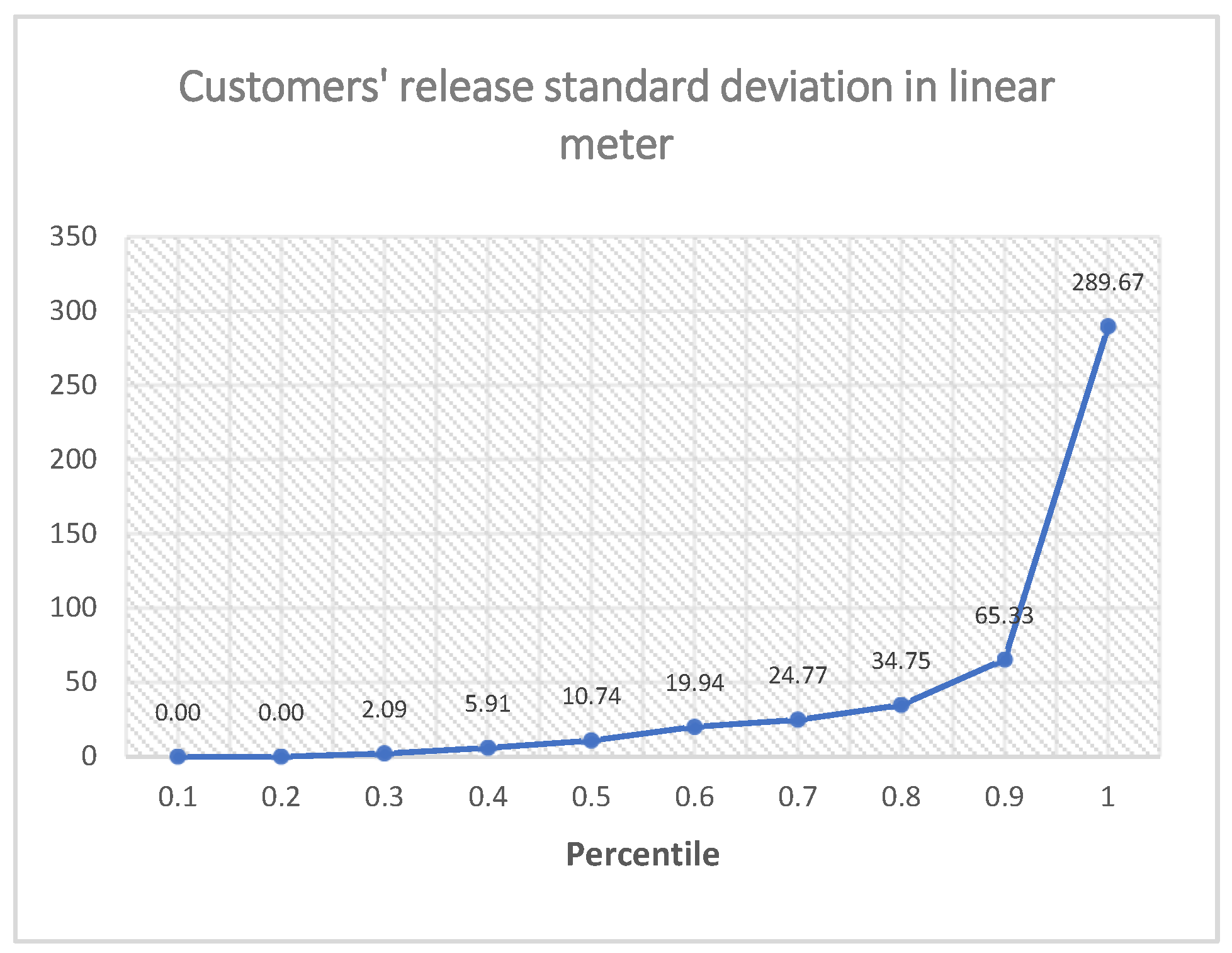
For customers (c.f. Figure A3), the standard deviation is greater, which is normal given that volumes are greater than suppliers taken individually. Eighty percent of customers have a variation of less than 34.75 mL, which is equivalent to about three trucks, which is relatively low when put into perspective with the average release of more than 400 mL.
Based on these two indicators, with the exception of a few extreme points, we validate the use of average rates in short-term planning models.
Figure A3.
Release variability analysis for customers.
Fixed RTI inventory requirement formulation
We aim to formulate the fixed inventory requirement for an RTI of type to operate the forward flows. According to Little’s law [19], the average quantity of empty RTIs present at supplier over a given period is constant. It is equivalent to the average lead time spent by an empty RTI at the supplier’s site multiplied by the total average empty-RTI demand over this period (which is considered to be equivalent to the average quantity of loaded RTIs delivered by the supplier to all its customers):
At supplier , in order to constitute the delivery batches of loaded RTIs in the forward flows at the supplier , an additional inventory is needed; it is given by:
The quantity of loaded RTIs in transit on a given supplier–customer link depends on the customer’s demand for part. On average, over a given period, this can be calculated by taking the average transportation lead time multiplied by the average demand over this period:
By analogy to the suppliers’ site, the average quantity of loaded RTIs present at customer site over a given period is given by the average lead time spent by a loaded RTI on-site multiplied by the average release over this period:
Hence, the total fixed RTI inventory requirement is therefore given by:
Customer–Supplier Frequency model
Initialization
Initialize , , for all the customers–suppliers couples and RTI types, based on the optimal solution obtained with the Customer–Supplier Flow model.
Compute initial values of and for all RTI types.
Compute initial values of for all the customers–suppliers couples.
Iterations
While :
Find the customer–supplier couple such as is the maximum.
Increase the delivery frequency for the customer–supplier couple :
Update the delivery batches of all RTIs for the customer–supplier couple :
Update the variable inventory requirements of all RTIs:
Update the quantities in shortage of all RTIs:
Update values:
Update transportation costs:
Adaptation of the short-term planning models to integrate dedicated RTI flows
The first model to adapt is the Customer–Supplier Flow model. It needs to be remembered that the purpose of this model is to define the flows and return frequencies between customers and suppliers taking into account the pool and dedicated RTIs. For dedicated RTIs, as explained above, the flows (i.e., the quantities transported between each customer and each supplier for each dedicated RTI type) are predetermined. The impact of dedicated flows will only be on the return frequency. For this purpose, we adopt a two-step sequential model:
- The first step consists in optimizing the flows between the customers and the predefined suppliers by taking into account only pool RTIs (i.e., the demand of the suppliers and the release of the customers consider only pool RTIs). The output of this step is to obtain the pool RTI flows between customers and suppliers.
- The second step is to calculate the return frequency on each customer–supplier link. The return frequency must take into account the pool RTI flows defined in the previous step and the predefined dedicated RTI flows.
Remark: Another way to integrate the dedicated RTI flows would have been to inject the predetermined dedicated RTI flows into the flow model in order to define the pool RTI flows, taking into account the trucks that circulate to transport the dedicated RTI flows, to better optimize the transportation cost. This method has been tested: it allowed us to obtain better results in terms of transportation costs but it increased the empty-RTI inventory requirement. Indeed, in cases where we would have customer–supplier links with dedicated RTI flows of low volumes and over long distances, the flow model as we have defined it will try to amortize the transportation cost on these links by also transporting pool RTIs, which goes against the optimization of the in-transit inventory and leads to the increase of empty-RTI inventory requirement. Therefore, we have chosen to use the presented method with two steps.
We introduce two additional parameters:
: the set of dedicated RTI types.
: the average quantity of dedicated empty RTIs of type transported from customer to supplier (per period).
: the maximum quantity of dedicated empty RTIs of type that can be transported in a truck.
The first step is to optimize the pool RTI flows with the Customer–Supplier Flow model:
Subsequently, a second step is carried out to integrate the dedicated RTI flows into the return frequency calculation. The return frequency on a customer–supplier link is given by the round-up of the number of trucks needed to transport the pool RTIs and the dedicated RTIs:
Based on the results of the flow model, we calculate the associated empty-RTI variable inventory requirement for both pool and dedicated RTIs with the same formula used thus far.
The second model to be adapted is the Customer–Supplier Frequency model. For this model, the inputs are the pool and dedicated RTI flows ( and ) and the return frequencies () determined previously. The change would consist in taking the additional inputs related to the quantity of empty RTIs available for the reverse flows of the dedicated RTIs .
References
- Cars, Planes, Trains: Where do CO2 Emissions from Transport Come from? Our World in Data. 2020. Available online: https://ourworldindata.org/co2-emissions-from-transport (accessed on 9 November 2022).
- Lange, J.-C. Design and Management of Networks with Fixed Transportation Costs. Ph.D. Thesis, UCL-Université Catholique de Louvain, Ottignies-Louvain-la-Neuve, Belgium, 2010. [Google Scholar]
- Tancrez, J.-S.; Lange, J.-C.; Semal, P. A location-inventory model for large three-level supply chains. Transp. Res. Part E Logist. Transp. Rev. 2012, 48, 485–502. [Google Scholar] [CrossRef] [Green Version]
- Tornese, F.; Gnoni, M.G.; Thorn, B.K.; Carrano, A.L.; Pazour, J.A. Management and Logistics of Returnable Transport Items: A Review Analysis on the Pallet Supply Chain. Sustainability 2021, 13, 12747. [Google Scholar] [CrossRef]
- Kim, T.; Glock, C.H. On the use of RFID in the management of reusable containers in closed-loop supply chains under stochastic container return quantities. Transp. Res. Part E Logist. Transp. Rev. 2014, 64, 12–27. [Google Scholar] [CrossRef]
- Martínez-Sala, A.S.; Egea-López, E.; García-Sánchez, F.; García-Haro, J. Tracking of Returnable Packaging and Transport Units with active RFID in the grocery supply chain. Comput. Ind. 2009, 60, 161–171. [Google Scholar] [CrossRef] [Green Version]
- Accorsi, R.; Baruffaldi, G.; Manzini, R. A closed-loop packaging network design model to foster infinitely reusable and recyclable containers in food industry. Sustain. Prod. Consum. 2020, 24, 48–61. [Google Scholar] [CrossRef]
- Na, B.; Sim, M.K.; Lee, W.J. An Optimal Purchase Decision of Reusable Packaging in the Automotive Industry. Sustainability 2019, 11, 6579. [Google Scholar] [CrossRef] [Green Version]
- Cobb, B.R. Inventory control for returnable transport items in a closed-loop supply chain. Transp. Res. Part E Logist. Transp. Rev. 2016, 86, 53–68. [Google Scholar] [CrossRef]
- Fan, X.; Gong, Y.; Xu, X.; Zou, B. Optimal decisions in reducing loss rate of returnable transport items. J. Clean. Prod. 2019, 214, 1050–1060. [Google Scholar] [CrossRef]
- Achamrah, F.E.; Riane, F.; Sahin, E.; Limbourg, S. An Artificial-Immune-System-Based Algorithm Enhanced with Deep Reinforcement Learning for Solving Returnable Transport Item Problems. Sustainability 2022, 14, 5805. [Google Scholar] [CrossRef]
- Zhang, Y.; Chu, F.; Che, A. Closed-loop Inventory Routing Problem for Perishable Food with Multi-type Returnable Transport Items. IFAC-Pap. 2022, 55, 2828–2833. [Google Scholar] [CrossRef]
- Iassinovskaia, G.; Limbourg, S.; Riane, F. The inventory-routing problem of returnable transport items with time windows and simultaneous pickup and delivery in closed-loop supply chains. Int. J. Prod. Econ. 2017, 183, 570–582. [Google Scholar] [CrossRef] [Green Version]
- Soysal, M. Closed-loop Inventory Routing Problem for returnable transport items. Transp. Res. Part D Transp. Environ. 2016, 48, 31–45. [Google Scholar] [CrossRef]
- Tanksale, A.N.; Das, D.; Verma, P.; Tiwari, M.K. Unpacking the role of primary packaging material in designing green supply chains: An integrated approach. Int. J. Prod. Econ. 2021, 236, 108133. [Google Scholar] [CrossRef]
- Accorsi, R.; Baruffaldi, G.; Manzini, R.; Pini, C. Environmental Impacts of Reusable Transport Items: A Case Study of Pallet Pooling in a Retailer Supply Chain. Sustainability 2019, 11, 3147. [Google Scholar] [CrossRef] [Green Version]
- Bottani, E.; Casella, G. Minimization of the Environmental Emissions of Closed-Loop Supply Chains: A Case Study of Returnable Transport Assets Management. Sustainability 2018, 10, 329. [Google Scholar] [CrossRef]
- Lakhmi, N. Returnable Transport Items Flow Optimization with an Application to the Automotive Supply Chain. Ph.D. Thesis, Université Paris-Saclay, Gif-sur-Yvette, France, 2021. Available online: https://www.theses.fr/2021UPAST131 (accessed on 7 November 2022).
- Little, J.D.C.; Graves, S.C. Little’s Law. In Building Intuition: Insights from Basic Operations Management Models and Principles; Chhajed, D., Lowe, T.J., Eds.; International Series in Operations Research & Management Science; Springer: Boston, MA, USA, 2008; pp. 81–100. ISBN 978-0-387-73699-0. [Google Scholar]
Figure 1.
RTI flow planning issues.
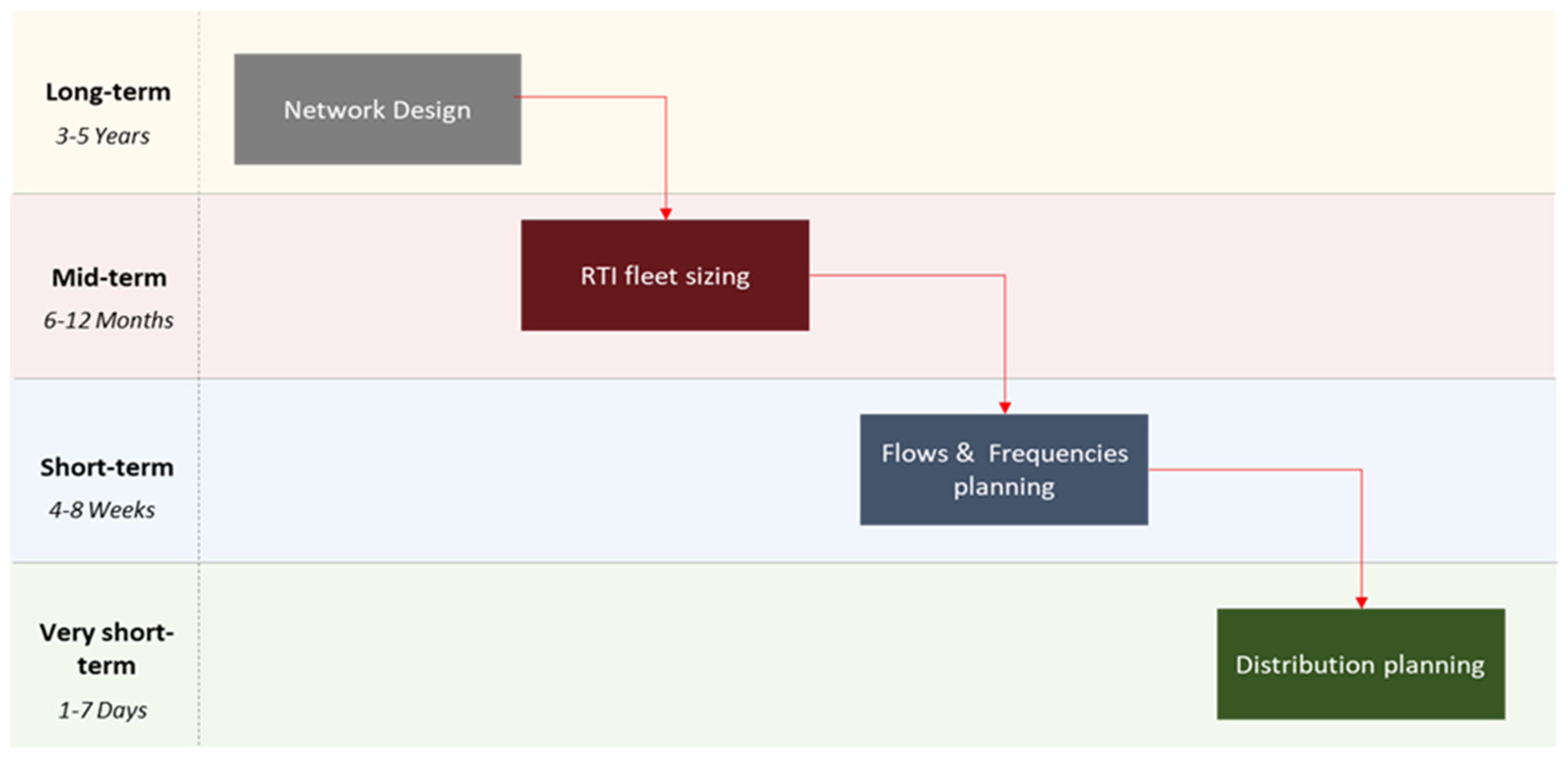
Figure 2.
RTI network.
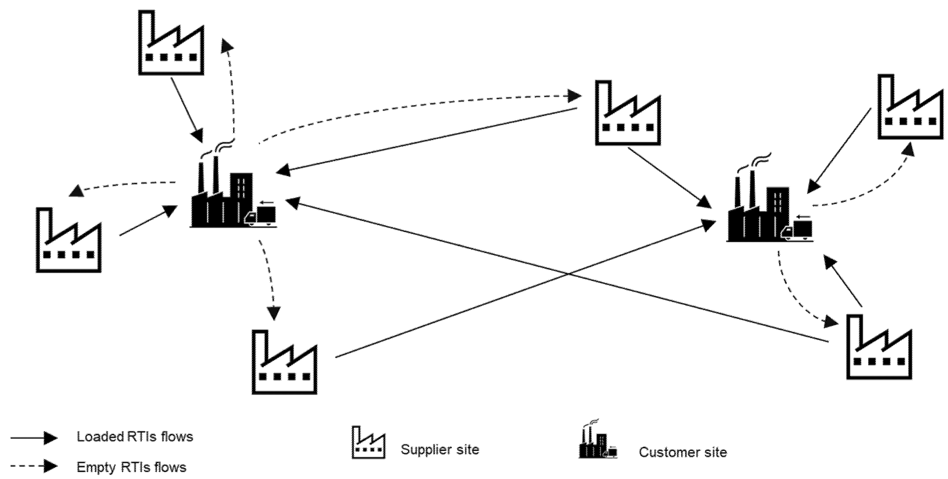
Figure 3.
Illustration of pool and dedicated RTI flow management.
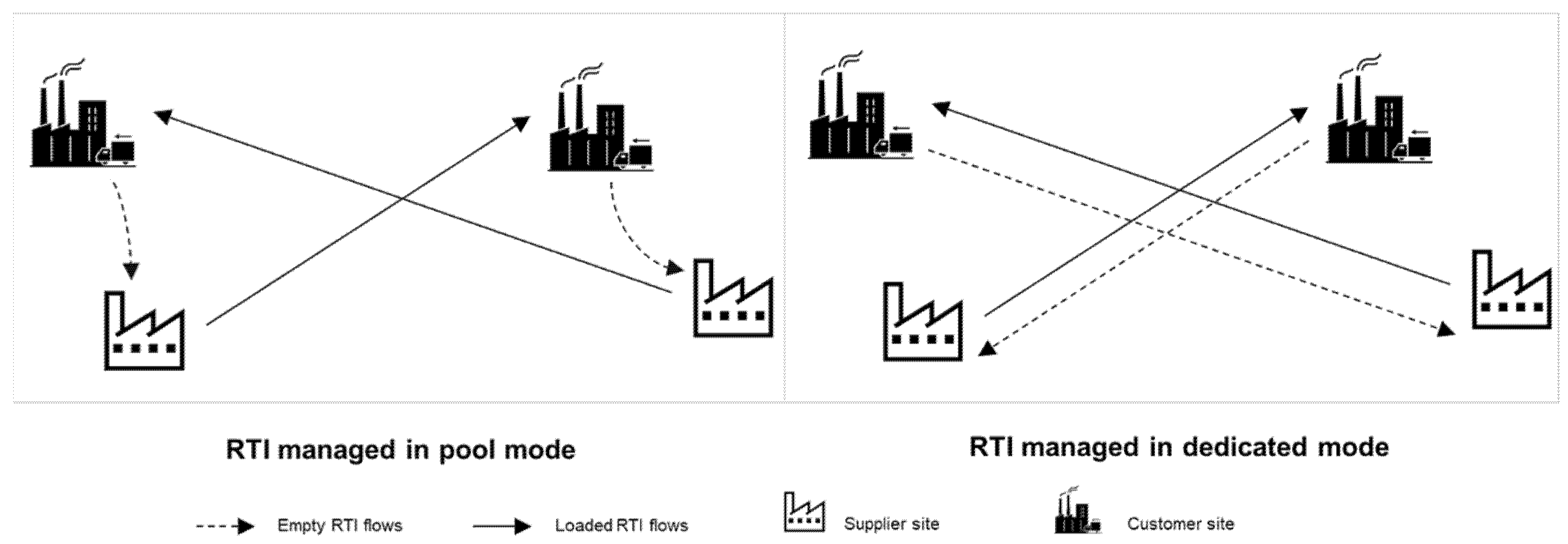
Figure 4.
RTI closed-loop supply chain (case of dedicated RTIs).
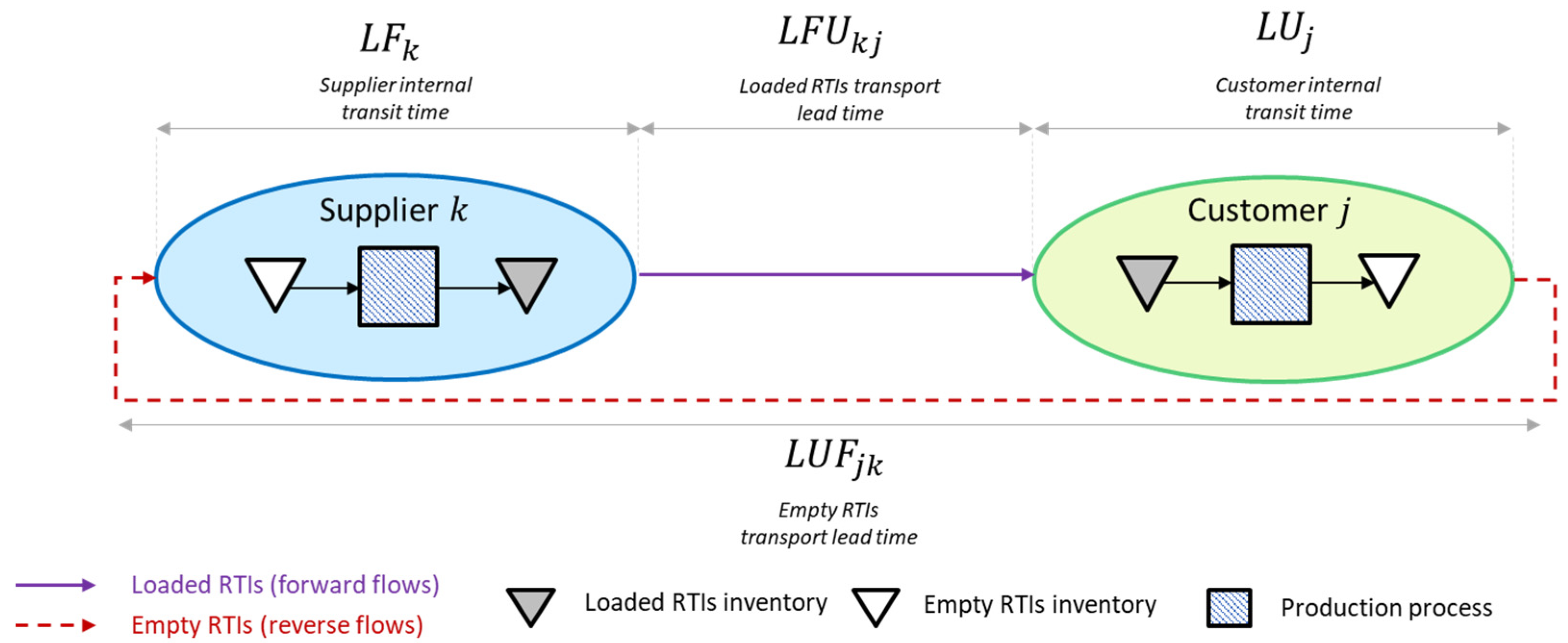
Figure 6.
Overall model pattern description with the main parameters and variables.
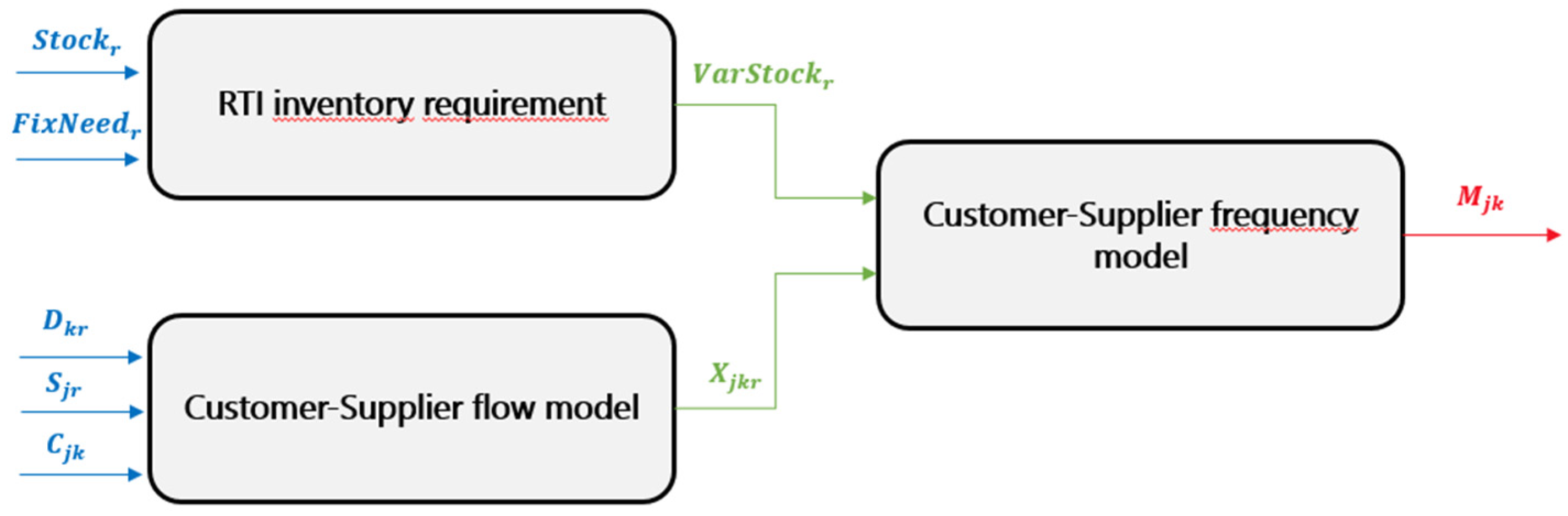
Figure 7.
RTI inventory requirement (case of pool RTIs).

Table 1.
Literature review summary.
| Research Paper | Objective | Perspective | Methodology |
|---|---|---|---|
| [2] | RTI flows and frequencies planning | Supply chain, single-RTI type | Optimization model |
| [3] | RTI flow design and management | Supply chain, single-RTI type | Review |
| [5] | Method for managing and evaluating the use of RFID in the tracking of RTIs | Single-supplier, single-customer, single-RTI type | Optimization model |
| [6] | Design and architecture of information systems for the pooling of RTIs | Supply chain, single-RTI type | Design approach |
| [7] | Design of RTI pooling network | Supply chain, single-RTI type | Optimization model |
| [7] | RTI fleet sizing | Single-supplier, single-customer, single-RTI type | Simulation model |
| [9] | RTI inventory management under uncertain returns | Single-supplier, single-customer, single-RTI type | Optimization model |
| [10] | RTI inventory management with RTI loss | Single-supplier, single-customer, single-RTI type | Optimization model |
| [10] | RTI inventory routing | Supply chain, multi-RTI type | Optimization model |
| [12] | RTI inventory routing | Single-supplier, multi-customer, multi-RTI type | Optimization model |
| [13] | RTI inventory routing with time windows | Single-supplier, multi-customer, single-RTI type | Optimization model |
| [14] | RTI inventory routing with uncertainty | Single-supplier, multi-customer, single-RTI type | Optimization model |
| [15] | RTI network design with green objectives | Supply chain, multi-RTI type | Optimization model |
| [16] | RTI flow design and management | Supply chain, single-RTI type | Comparative analysis |
Table 2.
Comparison of current transportation routes vs. transportation routes obtained from short-term planning models for pool RTIs.
Table 2.
Comparison of current transportation routes vs. transportation routes obtained from short-term planning models for pool RTIs.
| Current Transportation Routes | Transportation Routes Obtained by Short-Term Planning Models | Gap % | |
|---|---|---|---|
| Number of trucks used | 1046 | 840 | −20% |
| Average distance per truck | 314 Km | 220 Km | −30% |
Table 3.
Results of Customer–Supplier Flow model.
| Configuration | Scenario 0 | Scenario 1 | Gap % |
|---|---|---|---|
| Transportation cost obtained with Customer–Supplier Flow model | 4299 k€ | 3941 k€ | 8% |
Table 4.
RTI variable inventory requirement.
| Configuration | Scenario 0 | Scenario 1 | Gap % |
|---|---|---|---|
| RTI variable inventory requirement | 920,803 | 835,333 | 9% |
Table 5.
Results of Customer–Supplier Frequency model.
| Configuration | Scenario 0 | Scenario 1 | Gap% |
|---|---|---|---|
| Transportation cost obtained with Customer–Supplier Frequency model | 4338 k€ | 3944 k€ | 9% |
Publisher’s Note: MDPI stays neutral with regard to jurisdictional claims in published maps and institutional affiliations. |
© 2022 by the authors. Licensee MDPI, Basel, Switzerland. This article is an open access article distributed under the terms and conditions of the Creative Commons Attribution (CC BY) license (https://creativecommons.org/licenses/by/4.0/).
Share and Cite
MDPI and ACS Style
Lakhmi, N.; Sahin, E.; Dallery, Y. Modelling the Returnable Transport Items (RTI) Short-Term Planning Problem. Sustainability 2022, 14, 16796. https://doi.org/10.3390/su142416796
AMA Style
Lakhmi N, Sahin E, Dallery Y. Modelling the Returnable Transport Items (RTI) Short-Term Planning Problem. Sustainability. 2022; 14(24):16796. https://doi.org/10.3390/su142416796
Chicago/Turabian StyleLakhmi, Najoua, Evren Sahin, and Yves Dallery. 2022. "Modelling the Returnable Transport Items (RTI) Short-Term Planning Problem" Sustainability 14, no. 24: 16796. https://doi.org/10.3390/su142416796
Note that from the first issue of 2016, this journal uses article numbers instead of page numbers. See further details here.