Effects of Sea Breeze on Urban Areas Using Computation Fluid Dynamic—A Case Study of the Range of Cooling and Humidity Effects in Sendai, Japan

Abstract

Sea breezes have a significant influence on the urban environment of coastal cities. Therefore, the study of the sea breeze cooling range and its relationship with specific humidity is of great significance for improving the urban environment of coastal cities. This study aims to reproduce the climate of Sendai using the regional Weather Research and Forecasting (WRF) model, clarify the influence range of sea breezes in Sendai, and create an urban environmental climate map. The results revealed a strong correlation between the measured temperatures and the calculated results, and that the cooling effect range of sea breezes was mainly concentrated in the coastal area. In addition, the temperature rise mitigation effect changed over time, and although the maximum mitigation effect range affected a part of the urban area, it did not reach the inland area. In comparison, the specific humidity increased over time from the coastal area to the inland area. It was found that sea breezes mainly affected a part of the urban area and coastal areas in terms of temperature, but affected inland areas in terms of specific humidity. The results show that the range of the cooling effect of sea breezes on temperature was only concentrated within 5 km of the coast; in terms of moderating the temperature rise, there was an effect within the area ~7 km from the coast. In terms of humidity, the effect of sea breezes occurred approximately 1 h later than the effect of temperature.

1. Introduction

According to the statistics of the United Nations (2019), it is estimated that by 2050, approximately 68% of the world’s population will live in cities. With accelerating urbanization [1], urban environments have produced a series of environmental problems, such as urban heat islands [2,3], enhanced precipitation [4], and air pollution [5]. Global warming has become a worldwide problem, and the intensity and duration of high temperatures are increasing [6]. Due to the industrialization that has taken place since the last century, the extensive emissions of CO₂ have become the major source of anthropogenic greenhouse gas. This is the main trigger that contributes to global warming [7]. Urban sprawl has led to the formation of the urban heat island phenomenon. A 4 °C rise in temperature can be caused by the urban expansion in seen in Arizona, U.S.A., which has been illustrated by Georgescu et al. (2013) [8]. In the summer of 2018, there were approximately 90,000 heatstroke patients in Japanese metropolitan areas [9]. Therefore, it is urgent to take measures to alleviate such urban problems [10]. Improving the heat island effect has become a key challenge to achieve urban sustainability [11].

Most coastal cities have developed into megacities owing to their superior geographical location and convenient transportation amenities [12]. Wind is the movement in the horizontal direction of the atmosphere caused by the difference in atmospheric pressure [13]. During the day, the hot air on the land surface rises, and the cold air on the sea surface flows toward the land to supplement it, thus forming a sea breeze. Sea breezes can effectively alleviate the urban heat island (UHI) effect [14,15], and their cooling effect not only improves human comfort levels, but also effectively reduces energy consumption [16].

For this reason, many scholars have conducted in-depth research on the basic characteristics of sea breezes and their relationships with the urban environment. In summer, sea breezes always prevail [17]. Due to the low-temperature sea breeze that provides convective cooling in coastal cities, the UHI effect of coastal cities is lower than inland cities [18]. There is an interactive relationship between urban heat islands and sea breezes. The authors of [19] found that the strengthening of the urban heat island effect in the morning led to the earlier appearance of sea breezes. The authors of [20,21] collated and analyzed observational data covering 21 years, and found that the higher the surface roughness of a city, the weaker the sea breeze blowing towards Shanghai. According to a combined analysis of measured and numerical simulations, [22] reported that the cooling effect of the southwest wind was more obvious. The authors of [23] selected a coastal residential area in Sydney, Australia, through mobile measurement, and found that sea wind could significantly increase relative humidity. In terms of research methods, Ashie et al. (2009) obtained the relationship between the urban structure and sea breeze cooling effect through computational fluid dynamics (CFD) and numerical simulation [24]. The method of analysis based on long-term measurement data is widely used. In [25], long-term multi-point measured temperature data were analyzed and wind regime data were observed, showing that the temperature mitigation effect associated with sea breezes arrived later the closer Sendai was to the inland region.

The Weather Research and Forecasting (WRF) model is a regional meteorological model developed by the National Centers for Environmental Prediction (NCEP) and the National Center for Atmospheric Research (NCAR). In recent years, this model has been applied in the fields of meteorology, architectural engineering, and agronomy. It has also been used for various research purposes in the field of built environments, such as future climate prediction and climate reproduction at the urban domain level. The WRF model can arbitrarily set data (e.g., land use, topography, atmosphere, and sea surface water temperature), and the grid size of the data must be considered according to the scope of calculation. The authors of [26] used the WRF model to simulate the future climate scenario of the Sydney area. The authors of [27] simulated the wind speed in the North Sea and Baltic Sea using the WRF model and found that the difference between the simulated and observed values was very low (3.2%). Thus, many studies have investigated the relationship between sea breezes and urban environment; however, little research has been undertaken regarding the extent of the impact of sea breezes on cities and the corresponding positive and negative impacts.

Sendai City is in northeastern Japan near the Pacific Ocean and has a subtropical monsoon climate (city latitude: 31°49′00.00″ N; city longitude: 130°18′00.00″ E). The total area of Sendai is approximately 786 km². According to statistics, the population growth rate is relatively high. From 2010 to 2015, the growth rate reached 3.46%, and the population reached 1.08 million in 2015 [28]. In the past 90 years, the deviation of the average annual temperature in Sendai City has increased by approximately 2 °C. In addition, in terms of health damage, many people suffer from heatstroke annually. In summer, the number of heatstroke patients tends to increase on days when the temperature rises sharply from the previous day or days when the highest temperature exceeds 30 °C. According to previous research [25,29], the days when the southeast wind blows in Sendai City (hereinafter referred to as “sea breeze days”) suppress the rise in temperature in Sendai City. Therefore, it is necessary to clarify the scope of the influence of sea breezes on Sendai.

This study adopts a CFD analysis method to range of cooling and humidity effects of sea breeze in Sendai City and creates the KLIMA-ATLAS. The “KLIMA-ATLAS” is a series of map sets based on the characteristics of cities, which can provide insight on the current situation of the urban thermal environment and air quality. It can also be used to discuss improvement plans [30]. The purpose is to find the symbiosis point between city and climate environment, so as to ensure the friendly development of urban and climate environment, and make the urban environment sustainable. This study finally makes the KLIMA-ATLAS for the range of cooling and mitigation effects of sea breeze on the city. Basic research was established to explore the relationship between the UHI effect and climatic conditions.

The results will help the government to formulate corresponding countermeasures for different regions and strive to be a climate-resilient city.

2. Materials and Methods

2.1. Steps of Study

The measured temperatures collected in our laboratory were used to examine the calculation results in detail. The temperature distribution, specific humidity distribution, temperature change amount, and specific humidity change amount were evaluated, and the cooling effect range of sea breezes, temperature rise mitigation effect, and specific humidity rise range were mapped from their change amounts.

The following steps were performed in this study:

(1)

Arrangement of measured data obtained using equipment at the research laboratory in Sendai. Simultaneous multi-point measurements of temperature and humidity were used to organize the relevant data of the selected target day and representative location.

(2)

Verification of the usability of the WRF model. A correlation analysis between the measured air temperature and WRF calculation results was carried out. According to the measured results of the multi-point simultaneous measurements, the temperature distribution map was created using ArcGIS Pro and compared with the temperature distribution map obtained from the WRF calculation results.

(3)

Using the values obtained from the calculation results of the WRF model, we conducted a climate analysis and interpretation of the temperature and specific humidity affected by sea breezes.

(4)

Mapping the cooling area.

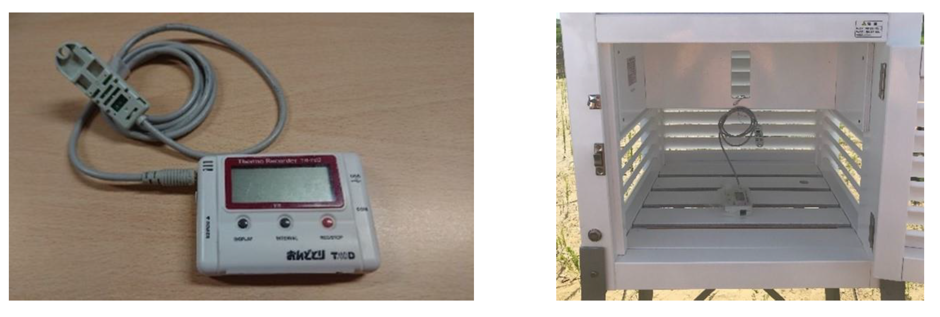
2.2. Measured Data

Data loggers with temperature and humidity sensors were installed on thermometer screens in multiple elementary schools and parks in Sendai City, and the measurements were performed under natural ventilation (Figure 1). The measuring instrument was a temperature and humidity recorder (T&D Corporation) (Figure 2). The test area was located as far away as possible in a place that could ensure all-day sunshine and avoid an unsuitable setting (e.g., the shade of trees). Among the collected data, the data from 22 August 2012 were used as the main analysis object.

Among the 23 points, point A was selected as a typical point of the inland area, point B was a typical point in the urban area, and point C was a typical point in the coastal area. Point A was located approximately 26 km from the coast, point B was located approximately 13 km from the coast, and point C was located approximately 4 km from the coast. Sendai is different from coastal cities, such as Hong Kong, because the urban area of Sendai is not close to the coastline; therefore, point B (~13 km away from the coast) is defined as an urban area or city center.

2.3. Model Setup

The CFD analysis used the regional WRF model to reproduce the climate of Sendai. As mentioned, the WRF model is a regional weather model of the NCEP and NCAR. The WRF model can arbitrarily set data (e.g., land use, topography, atmosphere, and sea surface water temperature), and the grid size of the data must be considered according to the scope of calculation. Table 1 presents the calculation parameterization.

Table 1. Calculation parameterization of the WRF model.

Calculation period	09:00 (JST) on 15 August 2012 to 09:00 (JST) on 25 August 2012
Vertical grid	30 layers
	Domain 1:9 km, dimension 37 × 28
Horizontal grid (Figure 3)	Domain 2:3 km, dimension 43 × 34
	Domain 3:1 km, dimension 31 × 28
Meteorological data	NCEP re-analysis of global objective data
Land data	Digital national land information (resolution of ~1000 m)
Microphysics	WSM 6-class graupel scheme
Radiation: Longwave	Rapid radiative transfer model
Shortwave	Dudhia shortwave
PBL scheme	Mellor–Yamada–Janjic TKE scheme
Surface scheme	Urban canopy model

Table 1. Calculation parameterization of the WRF model.

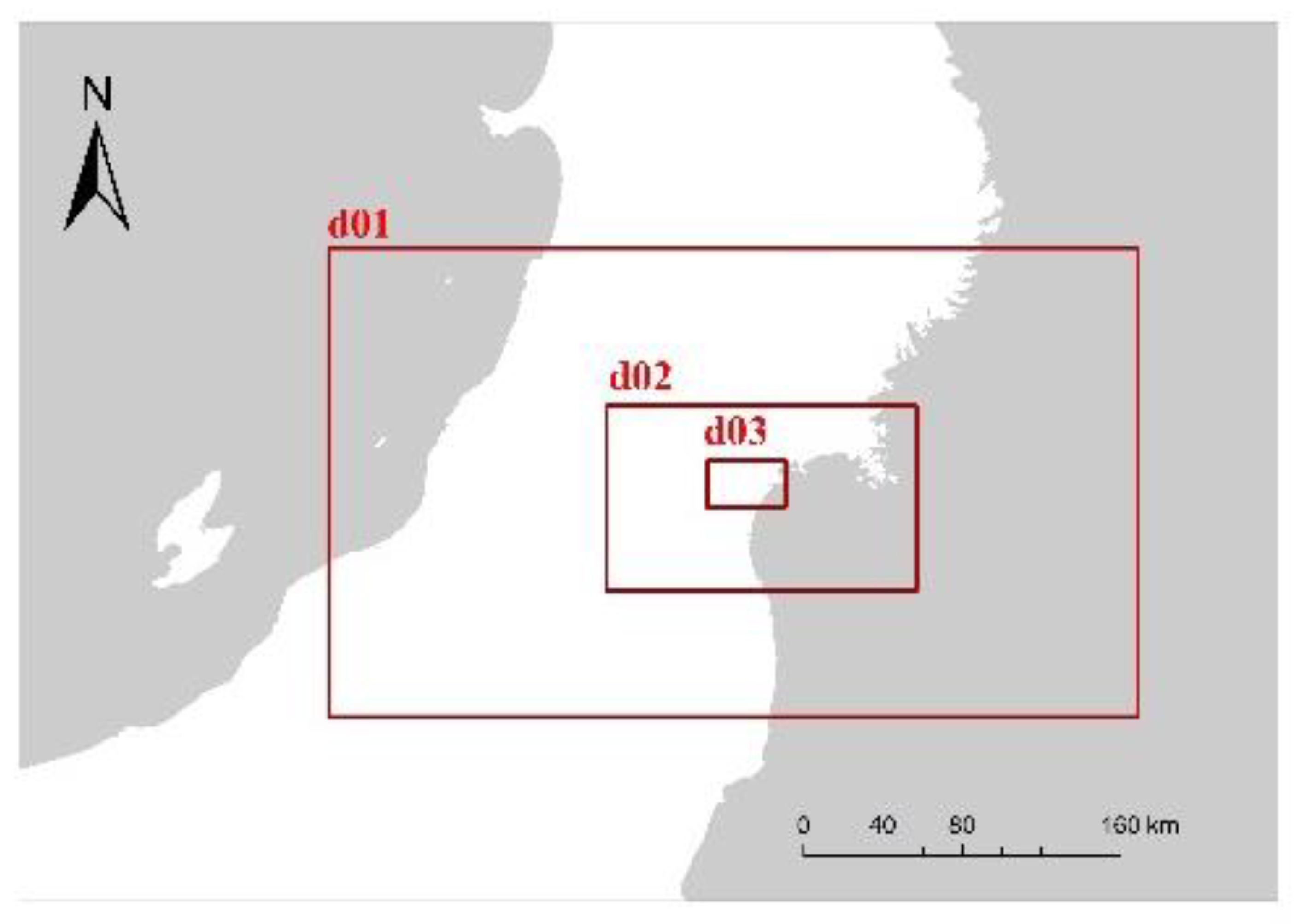
Calculation period	09:00 (JST) on 15 August 2012 to 09:00 (JST) on 25 August 2012
Vertical grid	30 layers
	Domain 1:9 km, dimension 37 × 28
Horizontal grid (Figure 3)	Domain 2:3 km, dimension 43 × 34
	Domain 3:1 km, dimension 31 × 28
Meteorological data	NCEP re-analysis of global objective data
Land data	Digital national land information (resolution of ~1000 m)
Microphysics	WSM 6-class graupel scheme
Radiation: Longwave	Rapid radiative transfer model
Shortwave	Dudhia shortwave
PBL scheme	Mellor–Yamada–Janjic TKE scheme
Surface scheme	Urban canopy model

Figure 4 shows the flow chart of the WRF modeling system. The steps of the run are as follows:

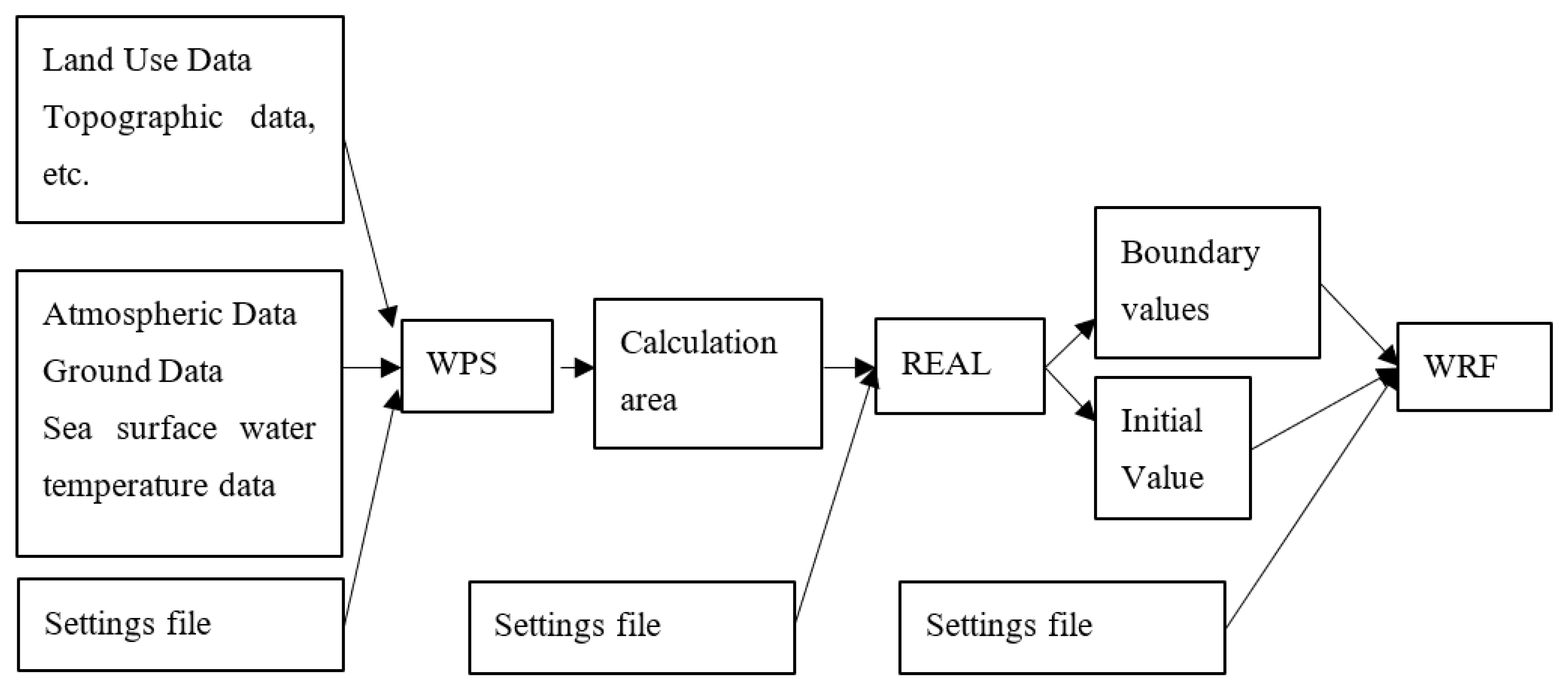
• Firstly, we run the pre-processing system, which is called WPS of the WRF. It should be noted that all the operations can be set in the “namenlist.wps”. This file contained four sections: “&share”, “&geogrid”, “& ungrib” and “&metgrid”. Additionally, these sections should be set one by one. As shown in the figure, it was necessary to define the area location of the study area. After that, we input the base data and set the number of nested domains according to the desired final WRF data resolution and input data resolution. At the same time, the domain size and data of the grid point were also set. This study area was located in Sendai, Japan. The source of the static land data was based on the United States Geological Survey (USGS). The download data were the data in 2014 with a resolution of 30 km. The final resolution was 1 km that was output from WRF. Therefore, we set 3 layers of nesting for this simulation.
• When the operation of pre-processing system was finished, the data that were generated by “&geogrid” and “&ungrib” were merged. As a result, the MET file can be generated. After that, we placed the MET file in the REAL file and created the data link. The WRF results of the three domains were obtained after editing the “namelist.input” and running the “REAL” system. The “namelist.input” contained six parts: “&time_conreol”, ”&domains”, “&physics”, ”&dynamics”, “&bdy_control”, and “&namenlist _quilt”. In the “&bdy_control” boundary control, the value of the specified area was set to 1, which is a default value. The value of the relaxation zone was set to 4, which is determined by the width of the boundary zone. The sum of these two values was the number of rows nudged by the specified boundary value. When we specified boundary conditions, it was only turned on (true) for domain 01, which meant that it must have been false for all other domains. The nested boundary conditions of all three domains were set to be true. The output files of the three domains were obtained after running the system.
• Finally, the calculation results were available after running the WRF system.

3. Results

3.1. Comparison of the WRF Model Results and Actual Measurement Data

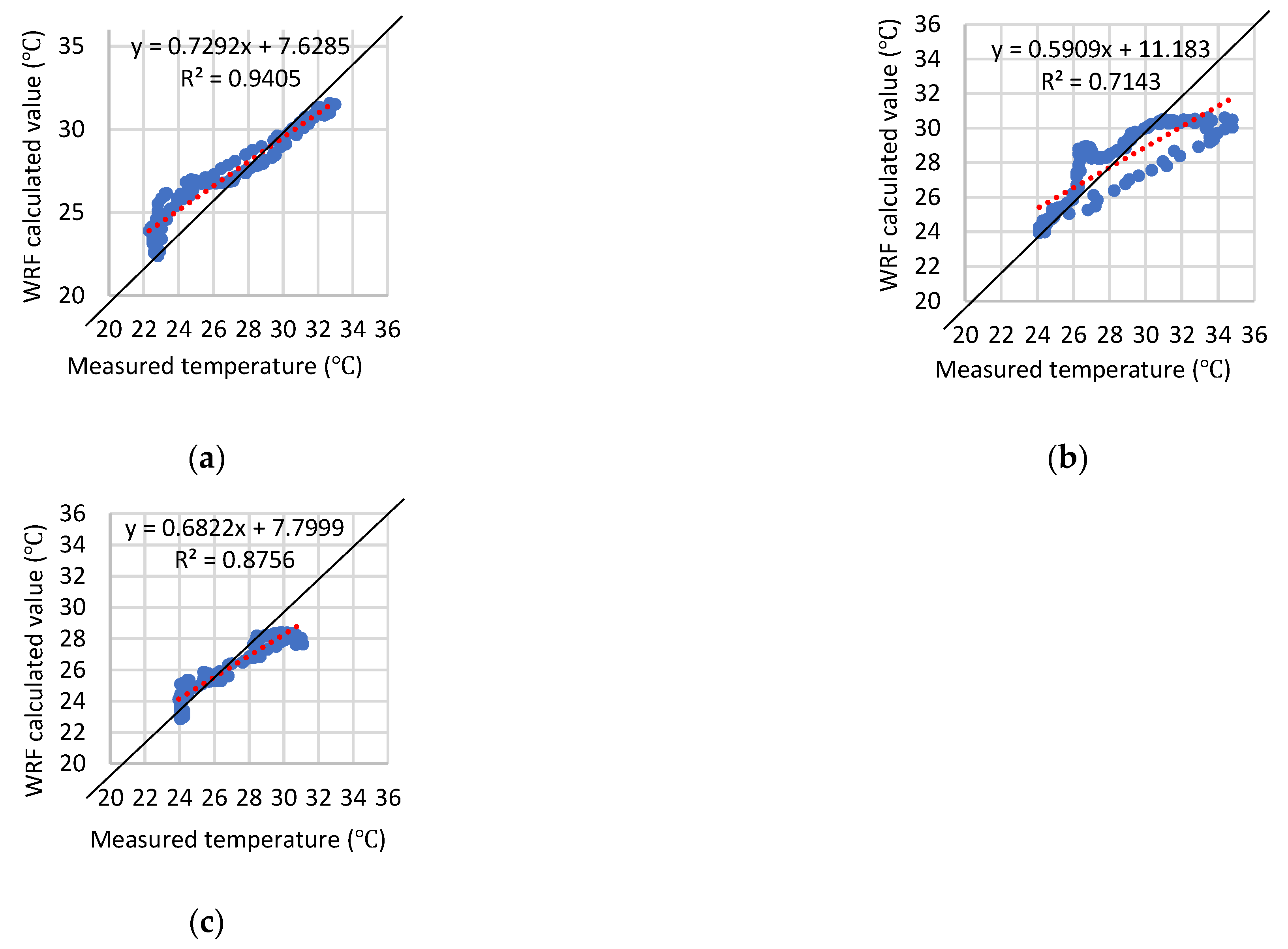
3.1.1. Temperature Correlation Analysis

As shown in Figure 5, a strong correlation was observed between the measured temperatures at any location and the calculated values of the WRF model. The correlation was particularly strong in coastal areas and strong inland areas. Although there were many underestimated values for the WRF calculations in the metropolitan area, a strong correlation was observed overall.

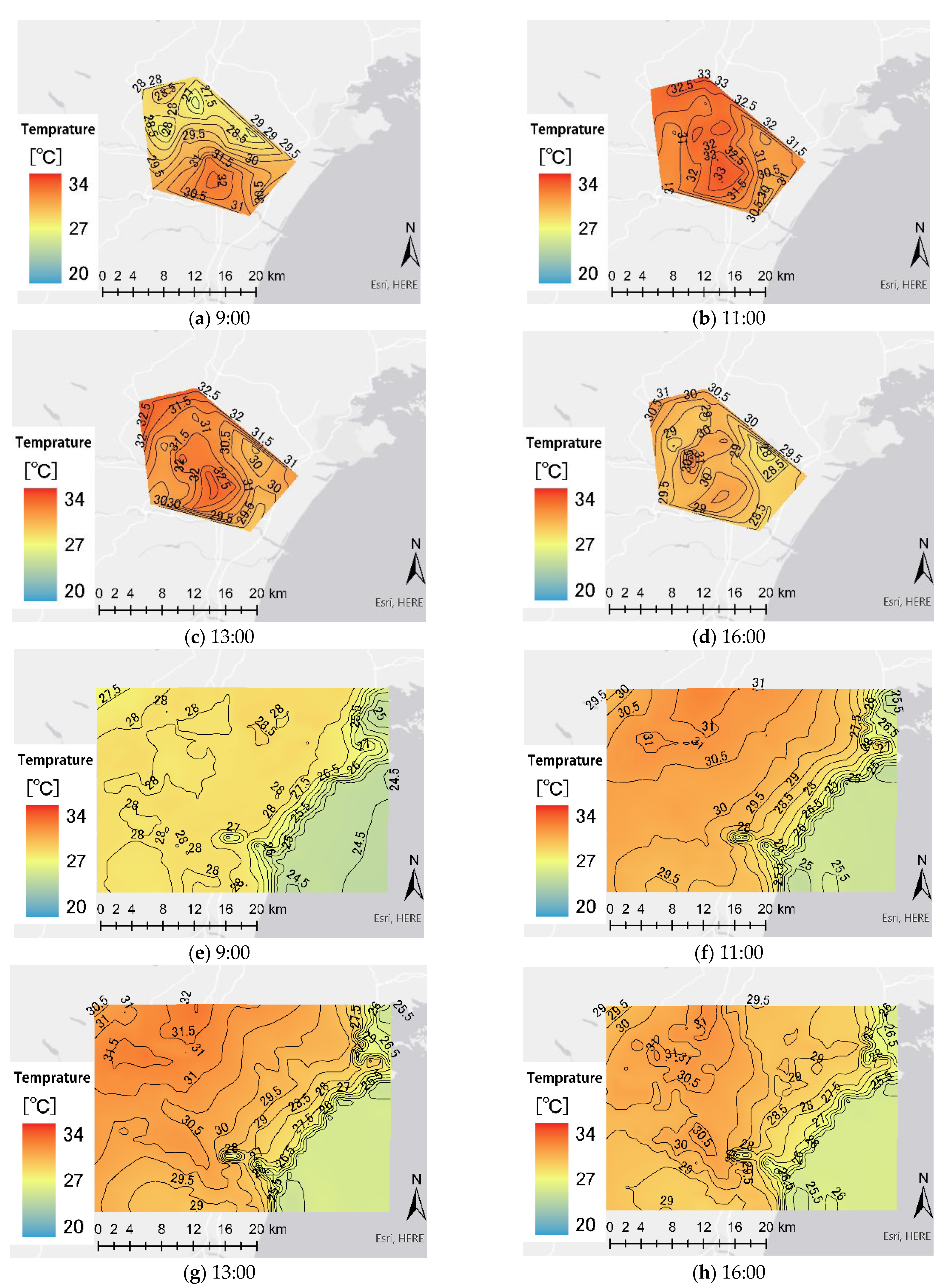
3.1.2. Comparison of Temperature Distributions

Based on the actual results of the simultaneous measurements at multiple points, a temperature distribution map was created using ArcGIS Pro1, and the results of the WRF model were also used to create a temperature distribution map. From these results, the temperature distributions were compared. The following three points were the main elements for comparison:

(1)

The temperature distribution in and around cities.

(2)

Did sea breezes affect the temperature rise from coastal areas to inland areas?

(3)

Was the temperature at the same level?

1 ArcGIS Pro is a GIS software provided by ESRI. A geographic information system (GIS) is a system for superimposing and displaying geospatial information on a computer, and is used for information visualization, information integration and analysis.

The results showed the following (Figure 6):

(1)

The measured temperature values started to increase from 08:00, with high temperatures starting to appear in urban areas, and lower temperatures in inland areas before 09:00, followed by a gradual increase in temperature from coastal to inland areas. The calculation results showed that the temperature values gradually increased from the coastal areas to the inland areas from 09:00, but the urban areas did not show extremely high temperatures.

(2)

Due to the mitigation effect of the sea breeze, the temperature measured at 11:00 showed that the temperature rise eased. It lasted until 13:00, when the easing effect began to decrease. The calculations showed that sea breezed had a moderating effect on the temperature rise from 09:00 onwards, with a gradual decline in temperature from inland to coastal areas. As for the measured temperature values, the rise in temperature was moderate along the coast before 13:00, but then reduced over time.

(3)

The calculations showed that, from 8:00 to 16:00, the temperatures were underestimated for the urban area, whereas the temperatures around it were similar.

From the above, it can be concluded that the results of these calculations were appropriate for the surrounding area, although consideration needs to be given to the higher temperatures in urban areas in the climate analysis.

3.2. Climate Analysis for Sendai

A climate analysis was performed using the data obtained from WRF calculations. The influence of sea breezes on temperature and specific humidity are discussed. Specific humidity is the humidity used in the meteorological field and is the mass of water vapor contained in 1 kg of moist air at a certain humidity. In engineering, humidity is defined as the absolute humidity, which is the mass of water vapor to 1 kg of dry air at a certain humidity.

$$\mathrm{S}=0.662\times \frac{\mathrm{e}}{\mathrm{p}-0.378\mathrm{e}}$$

$$\mathrm{X}=0.662\times \frac{\mathrm{e}}{\mathrm{p}-\mathrm{e}}$$

where S is the specific humidity, X is the absolute humidity, e is the water vapor pressure, and p is atmospheric pressure.

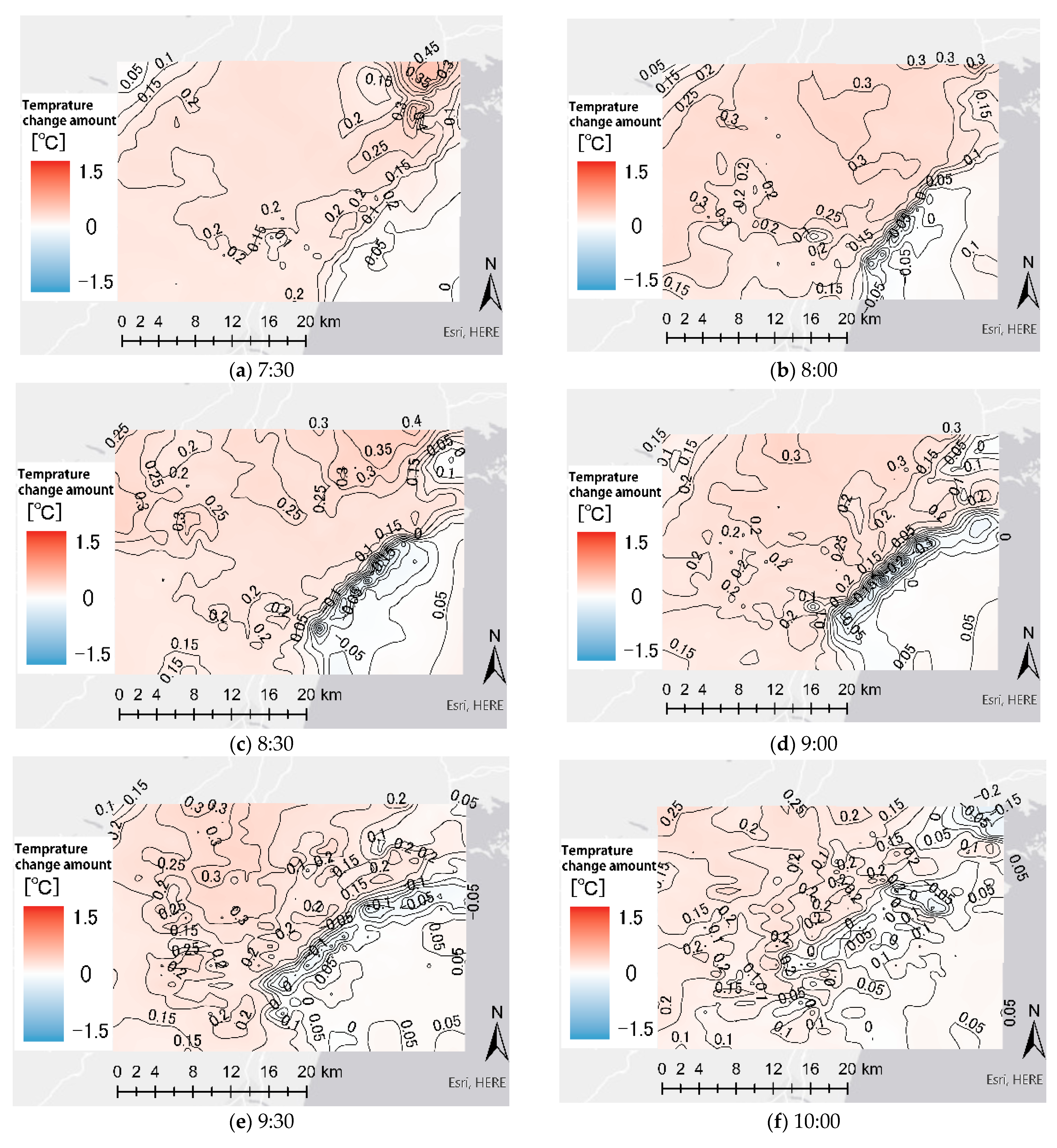
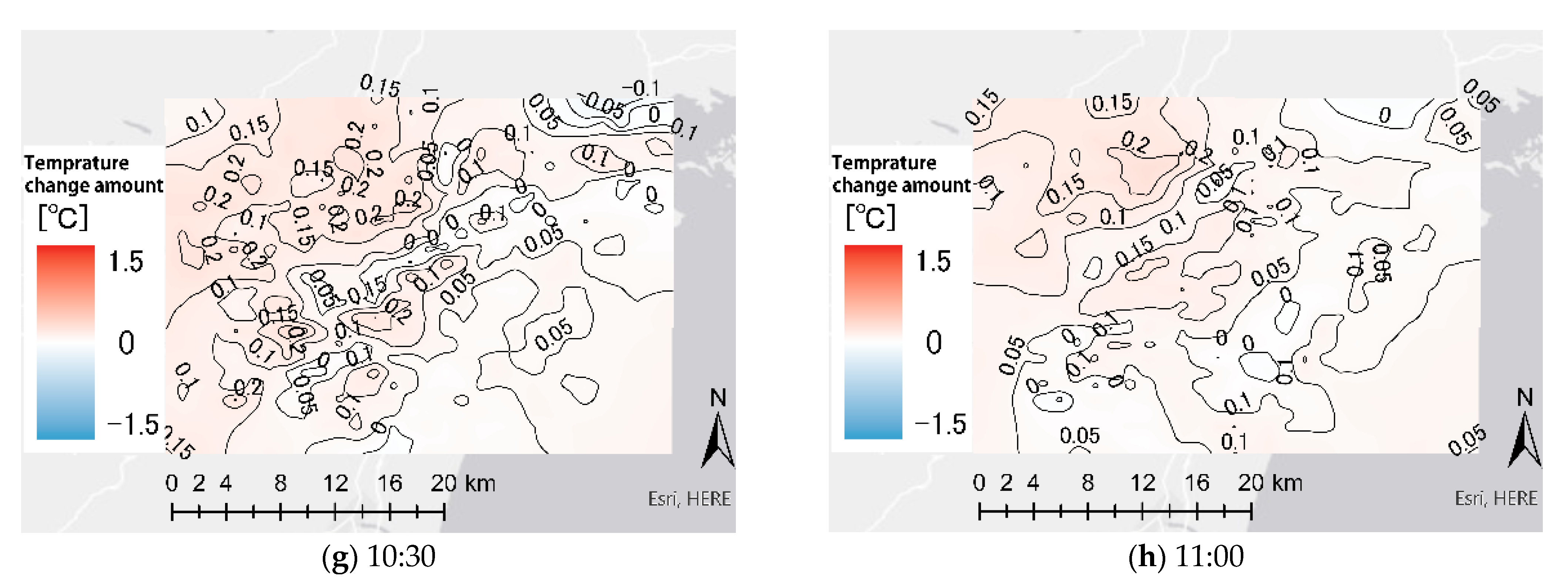
3.2.1. Trend of Temperature Difference

At 5:00, the temperatures values were relatively high in the city and by the sea, whereas they were particularly low in the north (Figure 7). However, from 9:00 onwards, the temperatures were positive in all areas except the coastal areas and seaside, and the temperature difference increased from 11:00 onwards. At 13:00, the temperatures showed positive values from the city to the inland area, especially in the inland area, which exceeded the average value (>2.5 °C). In addition, the range of ±0 expanded in coastal areas. At 16:00, the temperatures in the city and inland surrounding areas decreased, and by 18:00, the temperature gap decreased in all areas except the city and inland center area.

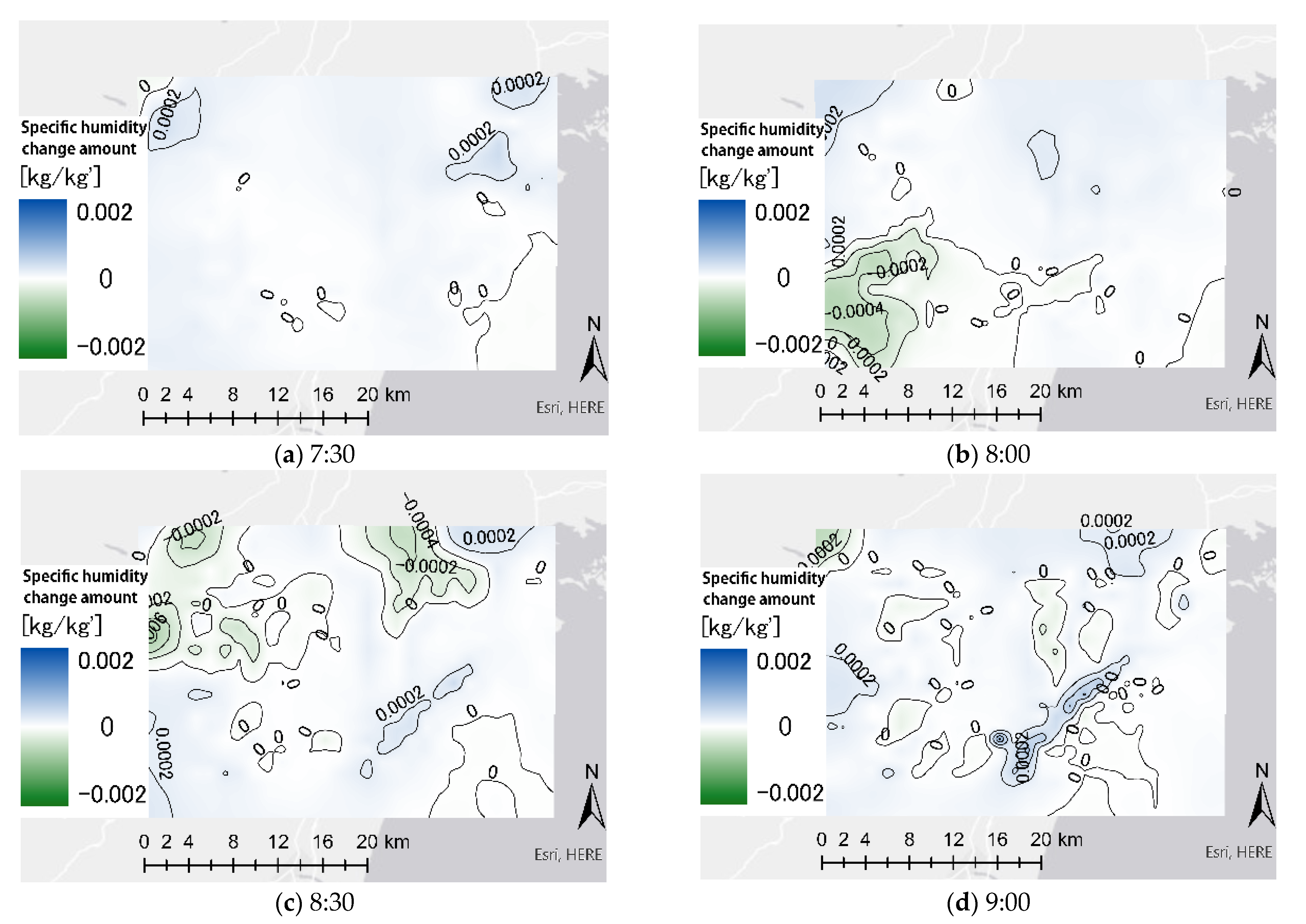
3.2.2. Trend of Specific Humidity Difference

Figure 8a for 5:00 shows that the specific humidity difference was lower with increasing distance inland, with coastal and urban areas being around ±0. From 9:00, the specific humidity difference increased, except in urban and central inland areas, and positive values were observed outside the coastal area. The specific humidity difference in the coastal area also increased. At 13:00, the specific humidity difference reduced in urban areas, and unlike the temperature difference, this did not result in a gradual reduction in coastal areas.

The range of the positive specific humidity difference in the coastal area increased at 16:00, and the difference between the coastal and inland areas increased. At 18:00, the specific humidity difference in some urban areas was ±0, and the specific humidity difference in areas outside the inland areas was positive.

3.2.3. Sea-Breeze-Induced Temperature Changes

At 07:30, the temperature rose by 0.15–0.2 °C, except in some coastal areas and inland areas (Figure 9). Ten minutes later, at 7:40, negative values were observed locally in the coastal areas, and these negative values gradually moved from the coastal areas to the urban areas and inland areas, where they remained until 9:30. Although it was 0 °C at 10:30, the temperature in the city no longer increased at 11:00, indicating that negative fronts could not be identified.

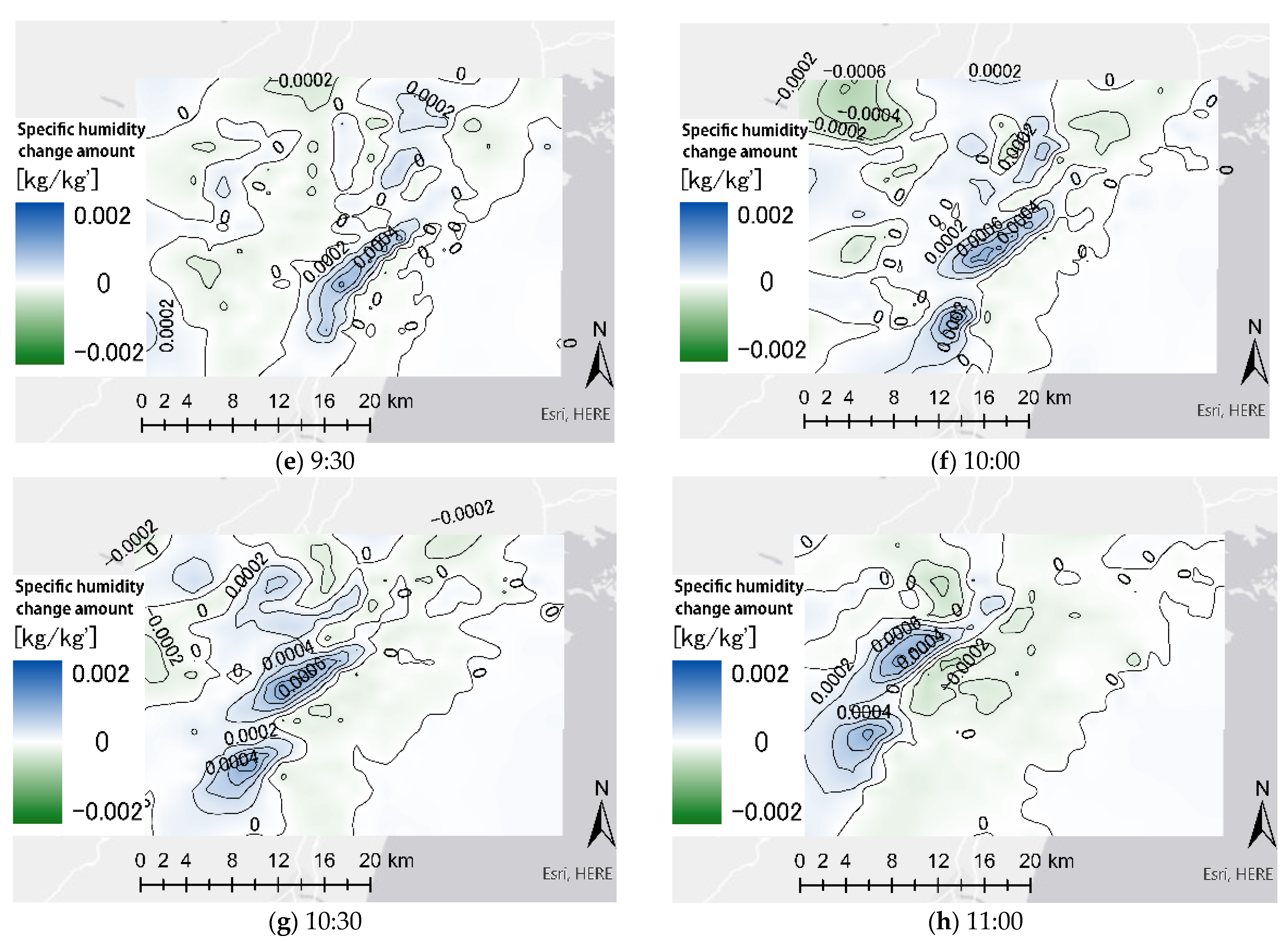
3.2.4. Sea-Breeze-Induced Humidity Changes

The overall humidity value was positive at 7:30, and negative values were observed from the southwest side at 8:00 (Figure 10). At 8:30, negative humidity values occurred in the interior and northeast regions, and the values around them were increasing. In addition, the humidity values of some coastal areas began to show localized increases. At 9:00, the locality of the positive humidity values increased, and the values rose in some coastal areas. At 9:30 and 10:00, the rising front gradually moved inland from the coastal areas. Unlike the change in temperature, a front with increasing values developed inland.

4. Discussion

4.1. Creating an Urban Environment KLIMA-ATLAS

The “KLIMA-ATLAS” is a series of map sets based on the characteristics of cities, which can provide insight into the current situation of the urban thermal environment and air quality. It can also be used to discuss improvement plans [30]. The Japanese Ministry of the Environment also stated that “The urban environmental climate map is a map group for exploring the improvement of the urban thermal environment and air quality. It consists of basic information and survey maps.” Currently, Japan is using KLIMA-ATLAS as a tool for urban and architectural planning, considering the protection of the natural environment and energy conservation. It consists of a climate analysis map and a planning guide map. The climate analysis map shows climatic zones, topographic classification by climatic characteristics, airflow, location of air pollution sources and pollution levels. In this section, we make the KLIMA-ATLAS for the range of cooling and mitigation effects of sea breeze on the city. Basic research was established to explore the relationship between the UHI effect and climatic conditions.

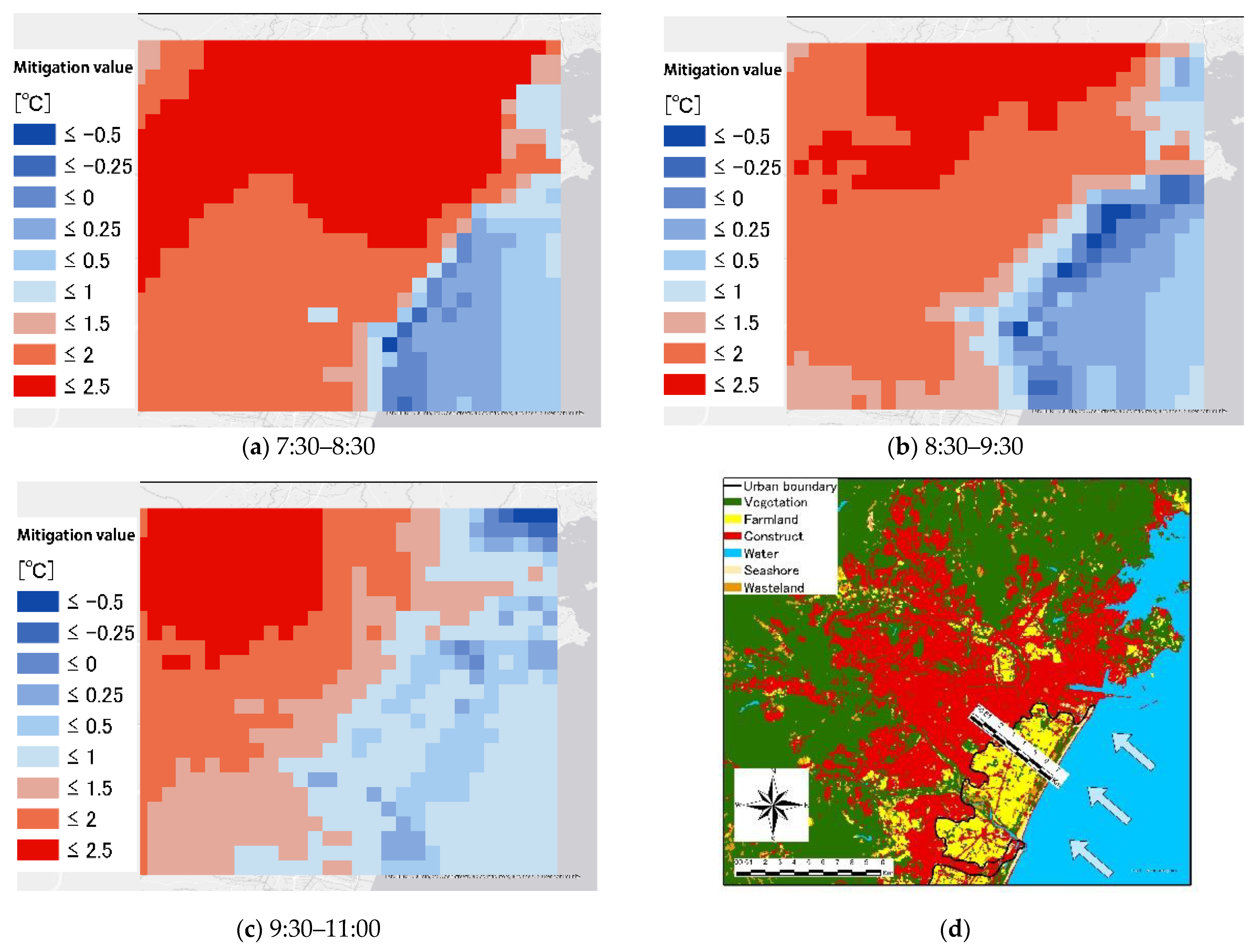
4.1.1. Range of the Cooling Effect of Sea Breezes

Section 3.2.3 analyzed the amount of accumulated change in cooling from 7:30 to 11:00 (Figure 11). The cumulative cooling value was only calculated for the temperature values that were negative before changing within 10 min. The result is a cooling effect close to −1 °C around the land–sea boundary next to the coast. In addition, the range with a cooling effect of −0.1 °C or more was concentrated in the coastal area, and there was no cooling effect in the urban area. The cooling range is concentrated in the coastal area and the same conclusion was obtained by T. Kaoru MATSUO et al. (2016) [31].

4.1.2. Range of Mitigation Effects of Sea Breezes

To calculate the range of the mitigation effect of sea breezes, the amount of change within 10 min was accumulated for 3 h and 30 min (7:30 to 11:00; Figure 12). Most of these locations reached a change value of 2.5 °C or more, but from the calculated duration of 3 h and 30 min, there seemed to be no mitigation effect.

4.1.3. Range of Mitigation Effects per Hour of Sea Breeze

Accumulated at 1 h intervals, it can be observed that in the first hour from 7:30 to 8:30 when the sea breeze started to have an effect, the range that produced effects above 2.5 °C decreased, while the range that produced effects below 1 °C increased (Figure 13a). In addition, within the next hour (8:30–9:30), the range of effects producing less than 1 °C increased, as did the range of mitigation effects from 5 km along the coast (Figure 13b). During the next 1.5 h (9:30–11:00), a mitigation effect occurred and the affected range was within 7 km from the coastline to the inland, as shown in Figure 13c,d.

4.1.4. Summary of Cooling and Mitigation Effects

As mentioned in Section 4.1.1, the cooling effect of sea breezes was only observed in coastal areas. As mentioned in Section 4.1.2 and Section 4.1.3, the mitigation effect was not obvious from the calculated duration of 3 h and 30 min, while the range of mitigation per hour of sea breeze gradually increased over time. The maximum distance of impact eventually extended to the area ~7 km along the coast.

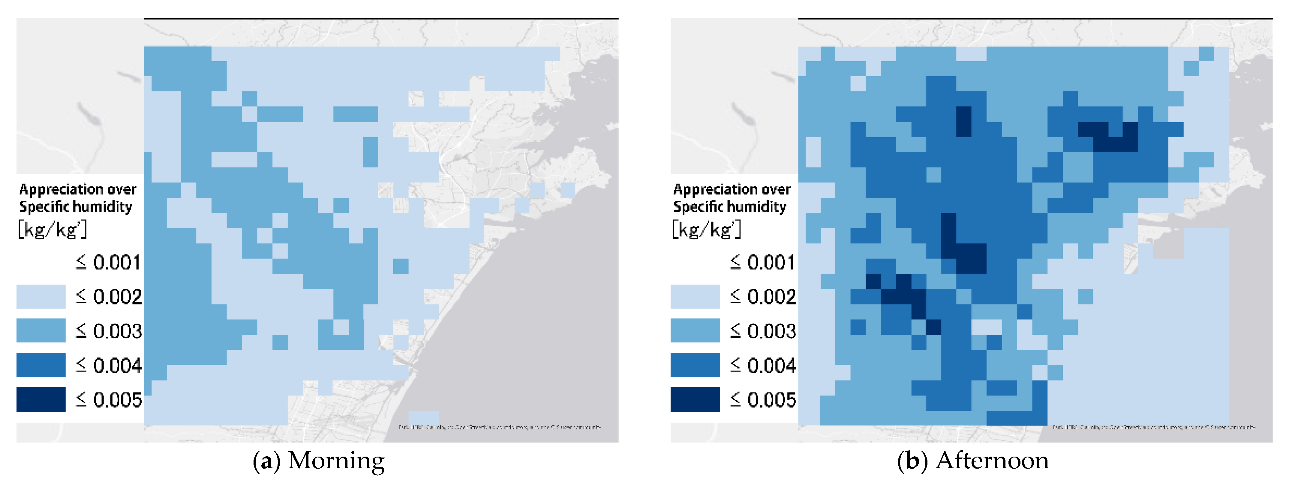
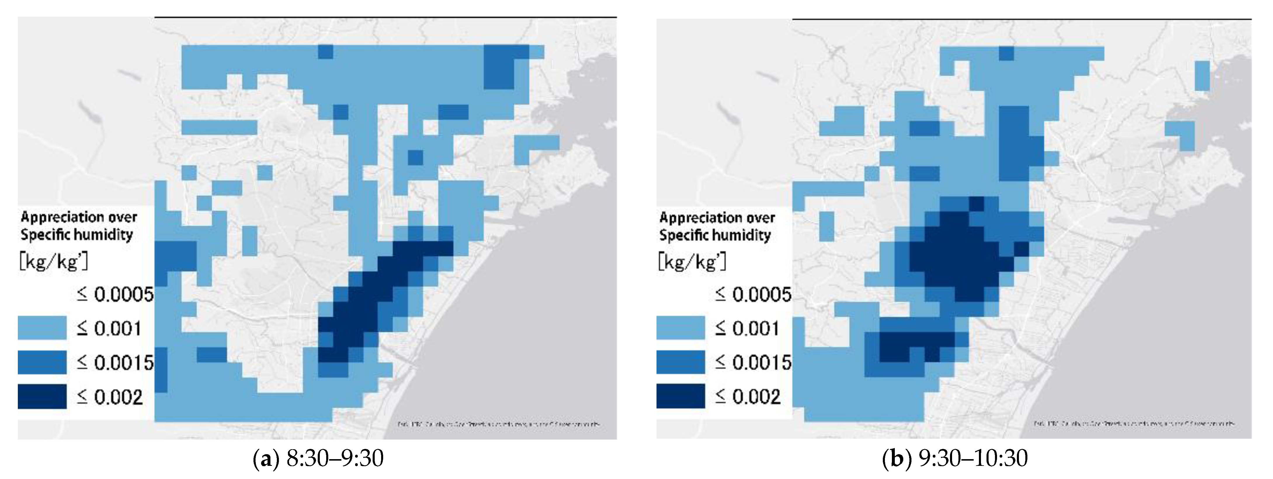
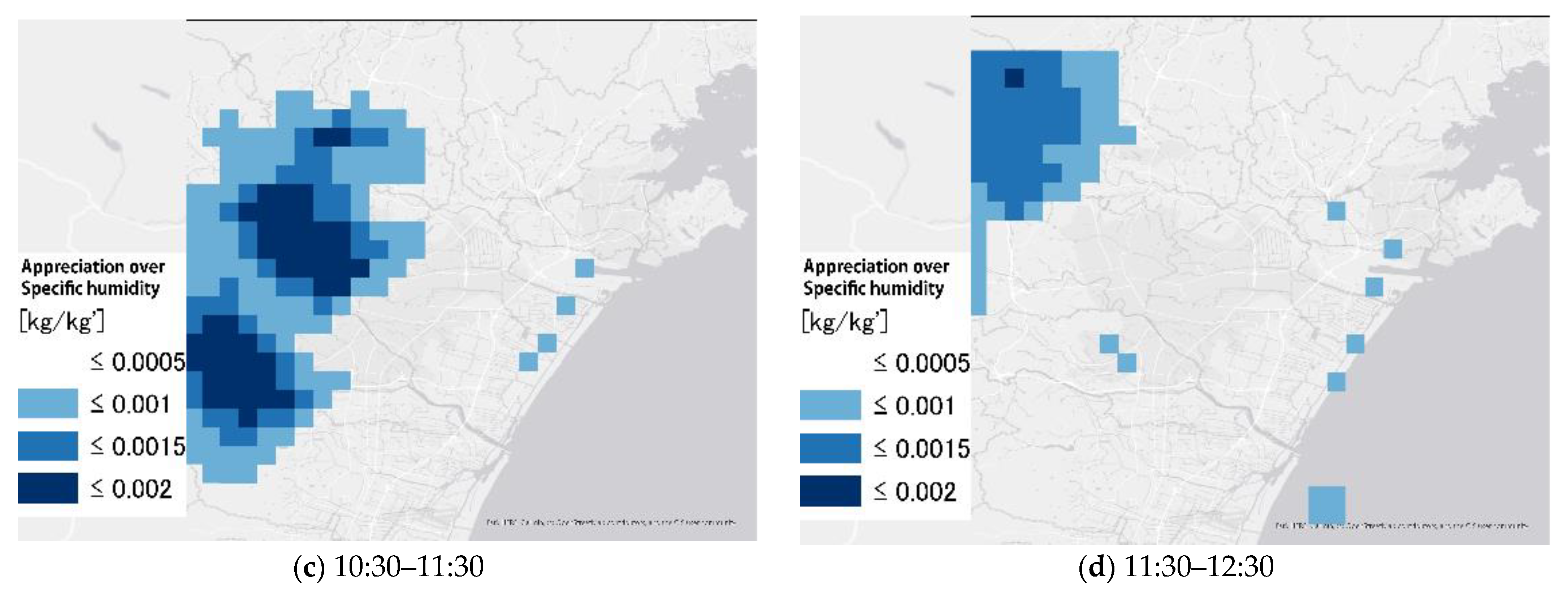
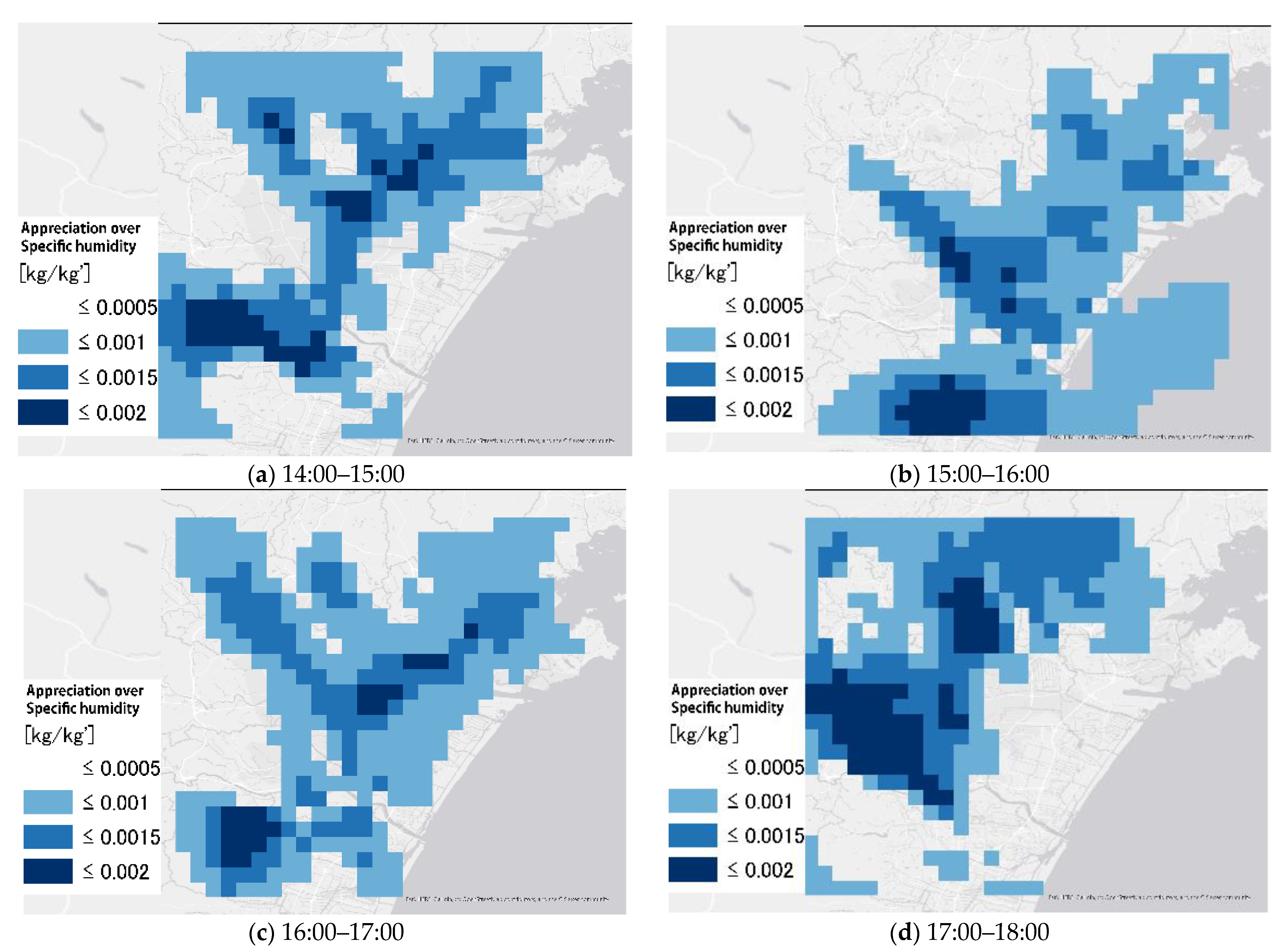
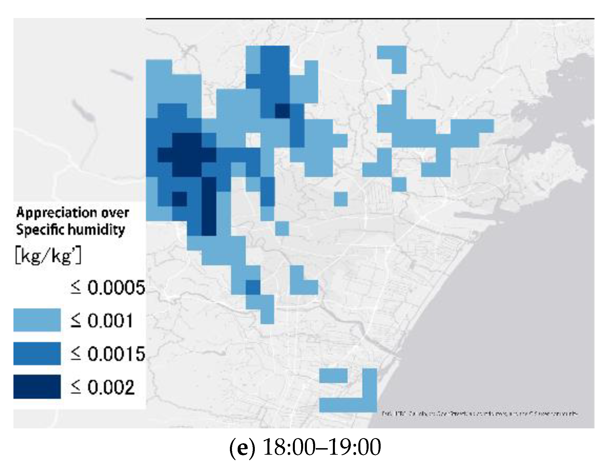
4.1.5. Range of Specific Humidity Rise Due to Sea Breezes

To calculate the magnitude of the specific humidity rise caused by sea breezes, we accumulated the specific humidity rise for the first 10 min of the 4 h period from 8:30 to 12:30 and 5 h period from 14:00 to 19:00. From 8:30 to 12:30, the specific humidity increased in the angle of the wind blown by the sea breeze (Figure 14a). Because the specific humidity near the land–ocean boundary was already high, the amount of increase was less, but there was an overall increase in specific humidity on the land side. From 14:00 to 19:00, an overall increase in specific humidity was observed, especially around the city (Figure 14b).

In addition, it can be seen from the hourly results that the specific humidity increase (in the morning and afternoon) gradually moved from the coast to the inland area (Figure 15 and Figure 16).

In this study, the regional WRF model was used to develop the urban environment KLIMA-ATLAS, and the influence range of sea breezes on temperature and humidity was analyzed. The results show that the range of the cooling effect of sea breezes on temperature was only concentrated within 5 km of the coast, and the cooling effect was not significant in urban and inland areas. However, in terms of moderating the temperature rise, there was an effect within the area ~7 km from the coast, and sea breezes also appeared to moderate the temperature rise in the city. In terms of humidity, the effect of sea breezes occurred approximately 1 h later than the effect of temperature. Moreover, the moderating effect of slowing down the temperature increase only occurred in the morning, while the humidity increased again in the afternoon. The rising effect of specific humidity reached the inland area, which was also influenced by sea breezes, but the range of the moderating effect of the temperature only appeared within the area ~7 km from the coast.

However, the WRF calculations could not reproduce the data of urban areas and yielded underestimated values compared with the actual measurements. Because the WRF model can set various boundary conditions, the range and effect of sea breezes could be visualized more precisely in the future by improving the reproducibility of the WRF model.

In addition, the values of wind direction and wind speed not covered in this study could be obtained in the same way as the temperature measurements. By confirming the reproducibility of the WRF model and the variation of wind speed in different regions, the time and scope of the arrival of sea breezes could be determined. Thus, it is believed that a more detailed urban environment KLIMA-ATLAS could be produced.

References

- Parnell, S.; Walawege, R. Sub-Saharan African urbanisation and global environmental change. Glob. Environ. Chang. 2011, 21, S12–S20. [Google Scholar] [CrossRef]
- Kusaka, H.; Hara, M.; Takane, Y. Urban Climate Projection by the WRF Model at 3-km Horizontal Grid Increment: Dynamical Downscaling and Predicting Heat Stress in the 2070’s August for Tokyo, Osaka, and Nagoya Metropolises. J. Meteorol. Soc. Jpn. 2012, 90B, 47–63. [Google Scholar] [CrossRef] [Green Version]
- Santamouris, M. Analyzing the heat island magnitude and characteristics in one hundred Asian and Australian cities and regions. Sci. Total Environ. 2015, 512–513, 582–598. [Google Scholar] [CrossRef]
- Seino, N.; Aoyagi, T.; Tsuguti, H. Numerical simulation of urban impact on precipitation in Tokyo: How does urban temperature rise affect precipitation? Urban. Clim. 2018, 23, 8–35. [Google Scholar] [CrossRef]
- Saitoh, T.S.; Shimada, T.; Hoshi, H. Modeling and simulation of the Tokyo urban heat island. Atmos. Environ. 1996, 30, 3431–3442. [Google Scholar] [CrossRef]
- Wang, S.; Zhu, J. Amplified or exaggerated changes in perceived temperature extremes under global warming. Clim. Dyn. 2019, 54, 117–127. [Google Scholar] [CrossRef]
- Onozaki, K. Population Is a Critical Factor for Global Carbon Dioxide Increase. J. Heal. Sci. 2009, 55, 125–127. [Google Scholar] [CrossRef] [Green Version]
- Georgescu, M.; Moustaoui, M.; Mahalov, A.; Dudhia, J. Summer-time climate impacts of projected megapolitan expansion in Arizona. Nat. Clim. Chang. 2013, 3, 37–41. [Google Scholar] [CrossRef]
- Japan Fire and Disaster Management Agency. The Emergency Conveyance Situation Due to Heat Stroke of 2018 (May to September); Japan Fire and Disaster Management Agency: Tokyo, Japan, 2018; p. 17. (In Japanese)
- Yamamoto, Y. Measures to Mitigate Urban Heat Islands. Environmental and Energy Research Unit. Quaterly Rev. 2006, 18, 65–83. [Google Scholar]
- Corburn, J. Cities, Climate Change and Urban Heat Island Mitigation: Localising Global Environmental Science. Urban Stud. 2009, 46, 413–427. [Google Scholar] [CrossRef]
- United-Nations. World Urbanization Prospects; Department of Economic and Social Affairs, United Nations: New York, NY, USA, 2018. [Google Scholar]
- Lutgens, F.K.; Tarbuck, E.J.; Tusa, D. The Atmosphere; Prentice-Hall: Englewood Cliffs, NJ, USA, 1995. [Google Scholar]
- He, B.-J. Potentials of meteorological characteristics and synoptic conditions to mitigate urban heat island effects. Urban Clim. 2018, 24, 26–33. [Google Scholar] [CrossRef]
- Hopkins, G.; Simmons, C.T. Atmospheres in a coastal city with a slope base setting. J. Geophys. Res. Atmos. 2016, 121, 5336–5355. [Google Scholar] [CrossRef]
- Lopes, A.; Lopes, S.; Matzarakis, A.; Alcoforado, M.J. The influence of the summer sea breeze on thermal comfort in Funchal (Madeira). A contribution to tourism and urban planning. Meteorol. Z. 2011, 20, 553–564. [Google Scholar] [CrossRef] [Green Version]
- Kolokotsa, D.; Psomas, A.; Karapidakis, E. Urban heat island in southern Europe: The case study of Hania, Crete. Sol. Energy 2009, 83, 1871–1883. [Google Scholar] [CrossRef]
- Liu, K.; Wu, Q.; Liu, J. Examining the association between social health insurance participation and patients’ out-of-pocket payments in China: The role of institutional arrangement. Soc. Sci. Med. 2014, 113, 95–103. [Google Scholar] [CrossRef] [PubMed]
- Khan, S.M.; Simpson, R.W. Effect of A Heat Island on the Meteorology of a Complex Urban Airshed. Bound. -Layer Meteorol. 2001, 100, 487–506. [Google Scholar] [CrossRef]
- Shen, L.; Zhao, C.; Ma, Z.; Li, Z.; Li, J.; Wang, K. Observed decrease of summer sea-land breeze in Shanghai from 1994 to 2014 and its association with urbanization. Atmospheric Res. 2019, 227, 198–209. [Google Scholar] [CrossRef]
- Dandou, A.; Tombrou, M.; Soulakellis, N. The Influence of the City of Athens on the Evolution of the Sea-Breeze Front. Bound. -Layer Meteorol. 2008, 131, 35–51. [Google Scholar] [CrossRef]
- Sasaki, Y.; Matsuo, K.; Yokoyama, M.; Sasaki, M.; Tanaka, T.; Sadohara, S. Sea breeze effect mapping for mitigating summer urban warming: For making urban environmental climate map of Yokohama and its surrounding area. Urban Clim. 2018, 24, 529–550. [Google Scholar] [CrossRef]
- He, B.-J.; Ding, L.; Prasad, D. Outdoor thermal environment of an open space under sea breeze: A mobile experience in a coastal city of Sydney, Australia. Urban Clim. 2020, 31. [Google Scholar] [CrossRef]
- Ashie, Y.; Hirano, K.; Kono, T. Effects of sea breeze on thermal environment as a measure against Tokyo’s urban heat island. In Proceedings of the Seventh International Conference on Urban Climate, Yokohama, Japan, 3–29 July 2009; pp. 29–32. [Google Scholar]
- Junimura, Y.; Watanabe, H. Study on the effects of sea breeze for decreasing urban air temperatures in summer. J. Environ. Eng. 2008, 73, 93–99. [Google Scholar] [CrossRef]
- Argüeso, D.; Evans, J.; Fita, L.; Bormann, K.J. Temperature response to future urbanization and climate change. Clim. Dyn. 2013, 42, 2183–2199. [Google Scholar] [CrossRef]
- Hahmann, A.N.; Vincent, C.L.; Peña, A.; Lange, J.; Hasager, C.B. Wind climate estimation using WRF model output: Method and model sensitivities over the sea. Int. J. Clim. 2014, 35, 3422–3439. [Google Scholar] [CrossRef]
- Statistics Bureau of Japan. Available online: http://www.stat.go.jp/english/index.html (accessed on 14 August 2021).
- Junimura, Y.; Watanabe, H. Actual condition of air temperature distribution in city and influence of wind upon the relationship between green coverage ratio and air temperature in summer season: Analysis based on the results of long-term multi-point measurements for coastal city Sendai in Tohoku region. J. Environ. Eng. 2007, 72, 83–88. [Google Scholar] [CrossRef] [Green Version]
- Environment Agency: 2002. Survey and Examination Business Report on Environmental Impact of the Heat Island Phenomenon. 2003; p. 3. Available online: http://www.env.go.jp/air/report/h15-02/ (accessed on 14 August 2021).
- Kaoru, T.M. Analysis on the Effect of Sea Breeze on Summer Diurnal Temperature Distribution Pattern in Hiroshima Plain: Mapping the Sea Breeze Effects for Mitigating Urban Warming; Architectural Institute of Japan: Tokyo, Japan, 2016; Volume 81, pp. 283–293. [Google Scholar]
Publisher’s Note: MDPI stays neutral with regard to jurisdictional claims in published maps and institutional affiliations. |
© 2022 by the authors. Licensee MDPI, Basel, Switzerland. This article is an open access article distributed under the terms and conditions of the Creative Commons Attribution (CC BY) license (https://creativecommons.org/licenses/by/4.0/).
Share and Cite
Peng, S.; Kon, Y.; Watanabe, H. Effects of Sea Breeze on Urban Areas Using Computation Fluid Dynamic—A Case Study of the Range of Cooling and Humidity Effects in Sendai, Japan. Sustainability 2022, 14, 1074. https://doi.org/10.3390/su14031074
Peng S, Kon Y, Watanabe H. Effects of Sea Breeze on Urban Areas Using Computation Fluid Dynamic—A Case Study of the Range of Cooling and Humidity Effects in Sendai, Japan. Sustainability. 2022; 14(3):1074. https://doi.org/10.3390/su14031074
Chicago/Turabian StylePeng, Shiyi, Yusuke Kon, and Hironori Watanabe. 2022. "Effects of Sea Breeze on Urban Areas Using Computation Fluid Dynamic—A Case Study of the Range of Cooling and Humidity Effects in Sendai, Japan" Sustainability 14, no. 3: 1074. https://doi.org/10.3390/su14031074