Intersection Signal Timing Optimization: A Multi-Objective Evolutionary Algorithm

Abstract

The rapid motorization of cities has led to the increasingly serious contradiction between supply and demand of road resources, and intersections have become the main bottleneck of traffic congestion. In general, capacity and delay are often used as indicators to improve intersection efficiency, but auxiliary indicators such as vehicle emissions that contribute to sustainable traffic development also need to be considered. It is necessary to evaluate intersection traffic efficiency through multiple measures to reflect different aspects of traffic, and these measures may conflict with each other. Therefore, this paper studies a multi-objective urban traffic signal timing problem, which requires a reasonable signal timing parameter under a given traffic flow condition, to better take into account the traffic capacity, delay and exhaust emission index of the intersection. Firstly, based on the traffic flow as the basic data, combined with the traffic flow description theory and exhaust emission estimation rules, a multi-objective model of signal timing problem is established. Secondly, the target model is solved and tested by the genetic algorithm of non-dominated sorting framework. It is found that the Pareto solution set of traffic indicators obtained by NSGA-III has a larger domain. Finally, the search mechanism of evolutionary algorithm is essentially unconstrained, while the actual traffic signal timing problem is constrained by traffic environment. In order to obtain a better signal timing scheme, this paper introduces the method of combining hybrid constraint strategy and NSGA-III framework, abbreviated as HCNSGA-III. The simulation experiment was carried out based on the same target model. The simulated results were compared with the actual scheme and the timing scheme obtained in recent research. The results show that the indices of traffic capacity, delay and exhaust emission obtained by the proposed method have more obvious advantages.

1. Introduction

With the quick development of science techniques and industrial society in China, the city population scale and city ground extend continuously. Produce and life are highly concentrated and cities develop quickly. However, with the rapid process of motorization, the demand for urban transportation is increasing. The original balance between supply and demand of urban traffic is broken, leading to worsening urban traffic congestion [1]. According to the United Nations Department of Economic and Social Affairs (DESA), more than 68% of the world’s population is expected to move to urban city areas by 2050 [2]. Because the feasibility to newly build or expand roads has become less and less, it is more important to improve the management and control of the traffic [3]. Transportation is one of the main contributors to global energy consumption, accounting for 29% of global energy consumption and 24% of global carbon dioxide emissions [4]. Low-speed driving and frequent start-up and parking increase energy consumption, carbon emission and pollutant emission. The frequent occurrence of traffic congestion is so damaging both to mobility and environment. It is expected that emissions will increase significantly in the next few years, further exacerbating climate change unless properly addressed [5]. In this situation, managing and mitigating traffic congestion is one of the great challenges for urban management [6]. Therefore, it is urgent to study intersection signal timing, improve intersection efficiency, make traffic infrastructure more convenient for users and make the environment sustainable.

According to the current situation of urban traffic control system, urban traffic control system can be divided into fixed time control, actuated control and adaptive signal control [7]. At present, most signalized intersections in developing countries such as China [8] and developed countries such as the United States [9] are equipped with fixed-time controllers and semi-actuated or actuated controllers. Usually, the effectiveness of the urban traffic control system depends on the performance of traffic dynamic evolution prediction model, traffic efficiency index model and its timing optimization method. Because the traffic demand is highly random, the intersection traffic signal timing problem (ITSTP) is a challenging and complex nonlinear problem for engineers and researchers [10]. Generally, the higher the accuracy of the model, the more complex the structure, and the more difficult it is to solve the optimal timing parameters. For the optimization methods, we distinguish and discuss the gradient based deterministic method and heuristic method. Since there are a large number of local optima in the signal timing solution space of ITSTP, the deterministic method is helpful to deeply understand the problem, but it is generally difficult to obtain an available solution in an affordable time [11]. Although heuristic methods such as genetic algorithm and fuzzy logic cannot provide the optimal solution, they are very useful for complex optimization problems when deterministic methods are difficult to calculate. Jin et al. [12] and Vogel et al. [13] developed a traffic light controller at isolated traffic intersections based on fuzzy logic. The results in terms of reducing congestion and travel time are very encouraging. However, according to [14,15], the traffic controller based on fuzzy logic and machine learning is not economically feasible and requires a lot of investment in configuration and maintenance. Evolutionary algorithms (EAs) are stochastic search methods that mimic the natural biological evolution and/or the social behavior of species [16]. The evolutionary algorithm has three main links: population maintenance in parallel optimization; each individual has a gene expression or coding, and the corresponding fitness value; each individual in the population can simulate gene changes through a series of different operations [17].

Traffic signal timing usually needs to deal with multiple conflicting targets. In order to enable decision makers to find the best solution, it is often inevitable to optimize multiple objectives at the same time. Many EAs are adopted to promote the smooth and efficient traffic operation at intersections. In the second part, we sort out and analyze the relevant research on traffic signal timing in recent years. Although previous studies considered multiple traffic efficiency indicators, most of them took traffic efficiency indicators as a single objective or converted multiple efficiency indicators into a single objective by weighting. The research on the efficiency improvement of intersection from the perspective of multi-objective has gradually become a research hotspot. Although for the traffic optimization problem, it is best to consider multiple objectives of multiple intersections at the same time, the multi-objective optimization problem of isolated intersections is the basis.

In order to optimize multiple objectives in ITSTP, it is usually necessary to establish a mathematical model of intersection traffic efficiency index to connect the optimization objectives with decision variables. After correctly expressing the problem and determining the decision variables, it is very important to design a multi-objective algorithm with good performance [18].The main contributions of this study are summarized in two aspects: (1) the total delay, vehicle emission and capacity are used as traffic efficiency indicators to establish a model, and the performance of common non dominated sorting algorithms NSGA-III and NSGA-II for solving multi-objective optimization problems in traffic signal timing is compared. It is found that NSGA-III has potential in diversity. (2) Aiming at the problem that the multi-objective optimization algorithm is easy to fall into the local optimum or the diversity becomes worse, and then the convergence becomes worse when solving the actual traffic signal timing problem, by combining the hybrid constraint strategy, the HCNSGA-III algorithm is proposed to avoid falling into the local optimum or improve the diversity to ensure the convergence. By comparing the algorithm with the recent traffic signal timing methods, the results show that the algorithm has better competitiveness.

The rest of this paper is structured as follows. Section 2 provides a detailed literature review on traffic signal timing optimization. Section 3 describes the study area and its data, and introduces the established model of optimization objectives, including constraint settings. Section 4 introduces the basic concepts of NSGA-III and constraint processing, and the basic steps of their combination. Section 5 details the results and discussion. Section 6 summarizes the main conclusions of this study and prospects for future research.

2. Related Work

Since the introduction of the simple automatic signal controller, the traffic signal control (TSC) System has been continuously improved to solve the problem of improving the level of TSC. In recent research, Jamal et al. selected average vehicle delay as the main performance index of the intersection and used GA and differential evolution (DE) algorithm to optimize the signal timing scheme to improve the service level of the intersection. The results show that although the DE converges to the objective function much faster, GA is better than DE in the quality of solution (i.e., minimum vehicle delay) [19]. However, as McKenney and White mentioned, there is no single absolutely dominant method for the study of ITSTP [20].

Table 1. Reported EAs approaches for the ITSTP.

Reference	Decision Variable(s)	Optimized Objective(s)	Problem Formulation	Solution Method
[21]	Vehicle routes. The green time for each traffic lights.	Time taken to dispatch vehicles.	Network-SO	Integer GA
[22]	Length of current green spit.	Total delay	Isolated-SO	Binary GA
[23]	The green light time. Phase differences.	The delay	Network-SO	Integer GA
[25,26]	Optimized cycle programs	Number of vehicles reaching their destinations. Global trip time.	Network-SO	Integer PSO
[27]	Green time of each phase.	Emissions. Total delay. Number of stops.	Network-MO as SO using weights	Integer GA
[28]	O-D multipliers. Cycle times. Stage green timings.	Network capacity. Vehicles emissions.	Network-MO as SO using weights	Continuous and integer
[33]	The green time for each phase.	Throughput. Queue length.	Isolated-MO	Real-coded NSGA-II
[34]	Signal cycle. Green time.	Per capita delay. Vehicle emission. Intersection capacity	Isolated-MO	Integer-IPSO

provides a comparative summary of applying EAs to ITSTP, including problem formulation and related solutions. It is hoped that it will be helpful for researchers to understand the research progress of ITSTP and better understand our work. Dezani et al. used GA to find the best route of vehicles at the same time and optimize the setting of green light interval of traffic signal in real time [21]. Jung et al. developed an ecological traffic signal system, in which a two-level optimization model was proposed [22]. The ecological signal operation layer is responsible for optimizing the total delay by manipulating the timing plan. The lower-level ecological driving algorithm layer optimizes the total fuel consumption by controlling the vehicle speed and acceleration. Li et al. used the green time and offset between intersections as optimization variables to control the 4-phase 3-intersections network and used the improved GA with conditional optimal retention strategy and adaptive mutation strategy to solve it. The experimental results show that compared with the standard genetic algorithm, the search time required by the algorithm is reduced by 38% and the number of iterations is reduced by 1/3 [23].

Particle swarm optimization (PSO) is a well-known algorithm, which can quickly converge to the appropriate solution [24]. In reference [25], PSO is used to find the optimal cycle plan (OCP) of all traffic lights in an urban area. The OCP is encoded as an integer vector, where each element represents the phase duration of a state of the traffic light. The fitness function is used to maximize the number of vehicles arriving at the destination and minimize the global travel time of all vehicles in the simulation time. The algorithm is applied to two large and heterogeneous metropolitan areas in Spain. The results show that compared with the deterministic algorithm, the number of vehicles arriving at the destination on time and travel time are increased by 0.13% and 15.7%, respectively. In Ref. [26], the authors extended the same work by comparing with the standard PSO and DE, in which their algorithm produced better results statistically.

However, most of the previous studies deal with the traffic signal control optimization problem from the perspective of single objective or double objective, without considering multiple objectives at the same time. There are studies on multi-objective optimization problems. In Refs. [27,28], the signal control multi-objective optimization problem is processed by using the weighted sum method. Its advantage is that it is simple to realize, only the scaled value is used to represent the original objective, and it is relatively easy to solve. The defect is that they are directly added by scaling and then weighting, which has a certain loss and omission of the information of the original target. In addition, the scaling process needs to know the target information in advance, such as maximum value, minimum value or average value, which is often difficult to determine. It is also difficult to know the user’s preference for different goals in advance. Even when the degree of preference is known, how to accurately formulate the weight is still a thorny problem, and it is difficult to ensure the Pareto solution set [29].

In reality, TST often needs to consider some different optimization objectives, such as vehicle delay, driving time, stops, queue length, fuel consumption, exhaust emission, etc., intended to find as many near optimal signal timing parameters as possible, which is related to a set of Pareto optimal solutions. NSGA-II [30] has better performance than other multi-objective evolutionary algorithms [31]. Among EAs, only GA has been successfully applied to commercial traffic signal control system [32]. NSGA-II is used in Ref. [33] to optimize supersaturated traffic signal intersections, with the goal of maximizing throughput and minimizing queue length. The simulation results show that compared with the commonly used signal timing optimization software Synchro, the timing scheme has good efficiency under the condition of supersaturation. In Ref. [34], a multi-objective optimization method is proposed by using Pareto optimization combined with PSO algorithm to optimize per capita delay, vehicle emission and intersection capacity. The algorithm is applied to a simple four-way intersection in Jinzhou, China. Compared with the solution generated by NSGA-II, the generated Pareto frontier solution has better consistency and diversity. In addition, under the same hardware environment, the calculation time of the algorithm is better than that of NSGA-II. When solving multi-objective problems with a large number of objectives, the increase in the number of objectives makes the number of non-dominated solution individuals in the population increase exponentially, which seriously weakens the ability of selection and search based on Pareto ranking, and the cost of measuring diversity becomes higher [35].

The framework of NSGA-III [36] is basically the same as that of NSGA-II. It also uses fast nondominated sorting to classify population individuals into different nondominated frontiers. The difference is that for environmental selection in the critical layer, NSGA-II uses crowding comparison operation to maintain diversity. The biggest change of NSGA-III is to change the crowding distance to the reference point method. The well distributed reference points are used to maintain the diversity of the population in the selection process. Based on the optimization objectives in the literature report, by paying attention to traffic and environmental problems to further solve the TST problem, we need to adopt more powerful optimization methods to balance diversity and convergence. In the fields of intelligent control and traffic optimization, many conditional constraints (constraints) are often encountered which bring great challenges to the solution of the problem [37,38]. However, the essence of EA is an unconstrained optimization technology. In order to better solve the complex constrained traffic signal optimization problem, a certain constraint processing mechanism must be combined. In recent years, researchers have proposed many constraint processing methods that combine constraints with evolutionary algorithms. According to the constraint processing mechanism in constraint optimization evolutionary algorithms, they can be divided into six categories [39] (penalty function method, feasibility rule, random sorting method, ε constraint processing method, multi-objective optimization method and hybrid method). It may be feasible to design a different constraint processing mechanism for different search states and adaptively select different constraint processing technologies [40,41].

3. Study Scenario and Data Description

In order to verify the effectiveness of this method in improving traffic efficiency at intersections, intersections with high-traffic pressure should be selected for testing. According to the survey, the total length of main roads and secondary roads in the main urban area of Jinzhou City (Liaoning Province, China) is 118.7 km, and the total length of branch road network is 110 km. The main urban area covers an area of 74.4 km². According to the calculation, the density of trunk road network is 1.60 km/km² and that of branch road network is 1.48 km/km². There is a large gap between the current road network density in the main urban area of Jinzhou City and the reasonable density recommended in the specification, especially the branch network density, which is still 1.52 km/km² lower than the offline recommended in the specification. The intersection used in this study is formed by the intersection of Shifu Road, an east-west trunk road, and Chengdu Street, a south-north secondary trunk road. Shifu Road is one of the main entrance and exit trunk roads in the urban area, and Chengdu Street is one of the main streets in the urban area. This intersection is a typical intersection in Jinzhou City. Its traffic efficiency and safety play an important role in whether the traffic flow in the suburban corridor is smooth. In addition, there are a large number of houses, businesses, schools and hospitals around the intersection. Therefore, it is necessary to evaluate the environment and optimize the signal control of the intersection.

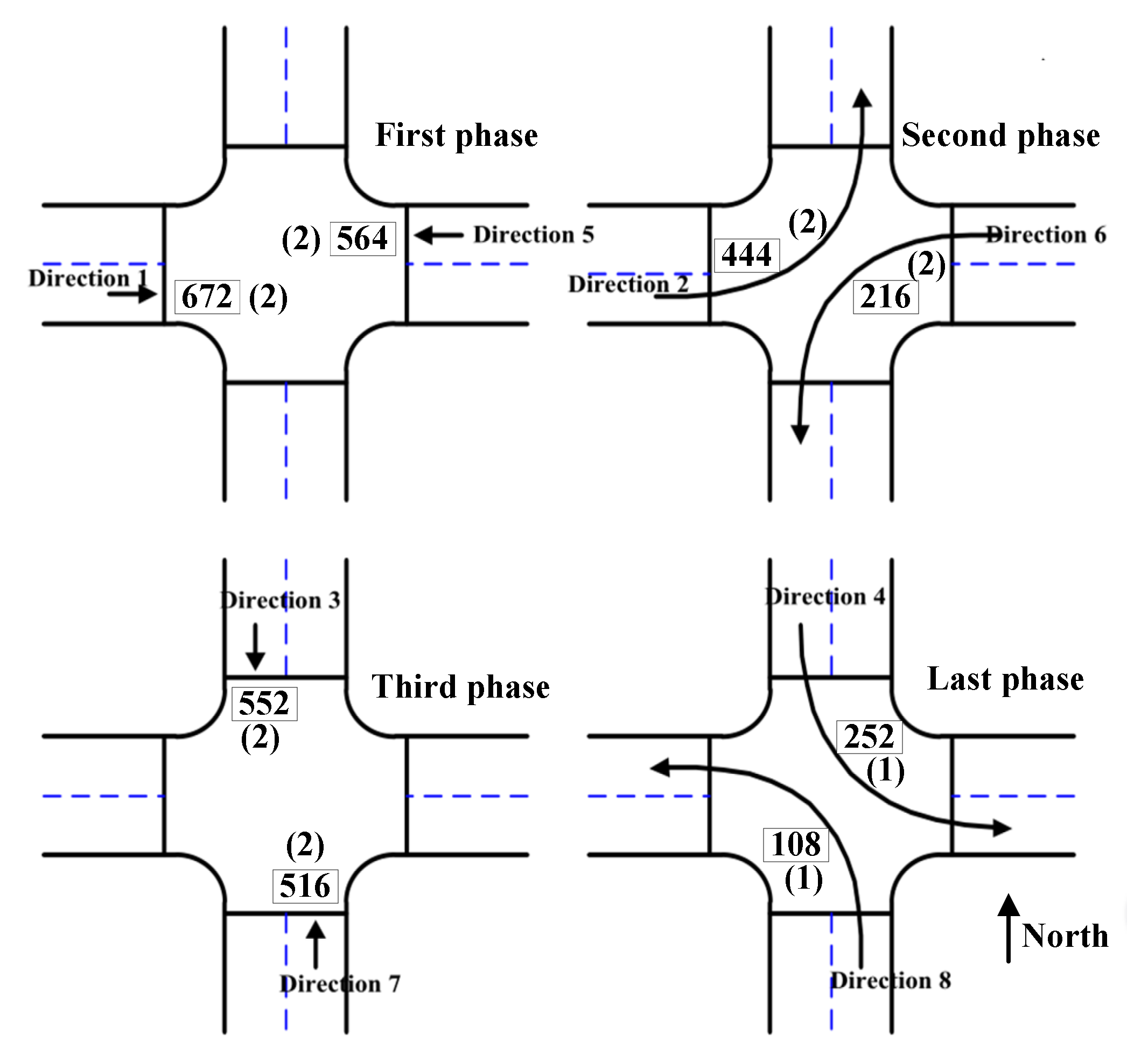
In addition, according to the survey of measured signal period, the signal control of the intersection is 4-phase timing. Each phase of the intersection consists of two opposite lanes, namely east-west straight, east-west left turn, north-south straight and north-south left turn. Among them, right turning vehicles are not controlled by a signal lamp. The phase sequence and corresponding traffic flow are shown in Figure 1. The traffic flow in each direction is framed with boxes, and the corresponding number of lanes is marked with brackets. In the original timing scheme, the green light time of east-west straight travel phase is 34 s, the green light time of east-west left turn phase is 30 s, the green light time of north-south straight travel phase is 41 s, the green light time of North-South left turn phase is 36 s, and the duration of the whole signal cycle is 161 s. The minimum green light time of the phase is 10 s, so that pedestrians have enough time to cross the road. The minimum cycle duration is 60 s and the maximum cycle duration is 200 s. The phase saturation of motor vehicles is set at 1200 pcu/h. The objective of exhaust emission is considered in this study. The emission factor of standard car exhaust is 5 g/(pcu·km), the standard car idle emission factor is 45 g/(pcu·h).

4. Methodology

Due to the limitation of traffic environment, traffic signal timing problem usually belongs to constrained multi-objective optimization problems (CMOPs). CMOP can be expressed by mathematical formula as:

$$\begin{array}{l}minimize [f\left(x\right) = \left(f_1\left(x\right),f_2\left(x\right),\cdots ,f_m\left(x\right)\right)]\\ subject to g_i\left(x\right) \le 0,i = 1,2,\cdots ,q\\ h_i \left(x\right) = 0,i=1,2,\cdots ,p\\ where x = \left(x_1,x_2,\cdots ,x_n\right) \in X\\ x = \left\{\left.x\right|l_k \le x_k \le u_k\right\} \in k = 1,2,\cdots ,n\\ l = \left(l_1,l_2,\cdots ,l_n\right), u = \left(u_1,u_2,\cdots ,u_n\right)\end{array}$$

(1)

where $f\left(x\right)$ is the output/objective function to be optimized, $g_i\left(x\right)$ represents the inequality constraint set and $h_i\left(x\right)$ represents the equality constraint. A constraint is a restriction that a variable can change. The variable $\left(x_1,x_2,\cdots ,x_n\right)\in R^n$ (solution space) is a control variable or a decision variable. By convention, optimization means a minimization problem, but it can also be designed as a maximization problem by negating the symbol of the objective function. The above optimization problem can be regarded as a decision problem, which involves finding the best vector of all control variables from the solution space.

In this study, NSGA-III algorithm and $\epsilon$ constraint optimization technology are used to take the total vehicle delay, capacity and exhaust emission of isolated signalized intersection as the objective function, and take multiple variables (i.e., traffic demand, existing phase scheme, split, saturated flow, etc.) as the input variables, which meet the traffic environment constraints. The green time of each signal phase and signal cycle length are decision variables or control variables. The main objective is to meet the traffic demand to the greatest extent and reduce pollution by selecting the best possible combination of signal timing plans. The following sections briefly summarize the objective functions and constraints to be optimized and introduce the principles of NSGA-III algorithm and ε constrained optimization technology, as well as the optimization steps for the current problems.

4.1. Construction of Optimization Objective Model

A multi-objective programming model is established based on the three objectives of delay, traffic capacity and exhaust emission. The objective function can be expressed as:

$$f\left(x\right) = min \left[D\left(x\right),-CAP \left(x\right), E\left(x\right)\right]$$

(2)

where: $D\left(x\right)$ is the total delay, $CAP\left(x\right)$ is the traffic capacity and $E\left(x\right)$ is the exhaust emission. The negative expression symbol before $CAP\left(x\right)$ does not mean that the value of $CAP\left(x\right)$ is negative but indicates the Pareto relationship between $CAP\left(x\right)$ and the other two goals.

• Delay at signalized intersection

This work adopts the total delay as the optimization objective of intersection delay, which can be written as follows:

$$D={\displaystyle \sum _i^N{V}_i{D}_i}$$

(3)

where $D_i$ is the average delay of each vehicle in the ith phase. ARRB model is a delay model of signalized intersection suitable for variable demand conditions [42]. $D_i$ can be written as follows according to this framework:

$$D_i={\displaystyle \sum _j^N\frac{c{⟮1-\frac{g_i}{c}⟯}^2}{2⟮1-\frac{q_{ij}}{S_{ij}}⟯}}+{\displaystyle \sum _j^N\frac{N_{ij}{x}_{ij}}{q_{ij}}}$$

(4)

$$N_{ij}=\left\{\begin{array}{c}\frac{S_{ij}{g}_i}{4}\left[\left(x_{ij}-1\right)+\sqrt{{\left(x_{ij}-1\right)}^2+\frac{12\left(x_{ij}-x_{ij0}\right)}{S_{ij}{g}_i}}\right],x_{ij}>x_{ij0}\\ 0,x_{ij}<x_{ij0}\end{array}\right.$$

(5)

$$x_{ij}=\frac{q_{ij}}{S_{ij}\cdot g_i}$$

(6)

$$x_{ij0}=0.67+\frac{S_{ij}{g}_i}{600}$$

(7)

where $D_i$ is the average delay of vehicles in ith phase, $V_i$ is the number of vehicles in ith phase, $c$ is the signal cycle length, $g_i$ is the effective green time in ith phase, $q_{ij}$ is the traffic volume of jth entrance lane in ith phase, $S_{ij}$ is the lane saturation flow of entrance jth lane in ith phase, $N_{ij}$ represents the number of vehicles stranded in unit time of jth entrance lane in ith phase and $x_{ij}$ is the traffic saturation flow rate of the jth entrance lane in the ith phase.

2.

Traffic capacity

The traffic capacity of signalized intersection is estimated according to each entrance lane of the intersection. The capacity of an entrance lane in one direction is the sum of the capacity of each lane of the entrance lane. The capacity of an entrance lane is multiplied by the green signal ratio of its signal phase based on the saturated flow rate of the lane. Expressed as:

$$CA{P}_i={\displaystyle \sum _j^{}{S}_{ij}{\lambda }_i}={\displaystyle \sum _j^{}{S}_{ij}⟮\frac{g_i}{C}⟯}$$

(8)

$$CAP={\displaystyle \sum _i^{}CA{P}_i}$$

(9)

where: $CA{P}_i$ is the capacity of ith entrance lane and ${\lambda }_i$ is the green signal ratio of the signal phase of ith entry lane.

3.

Vehicle emissions

Vehicle emissions at urban road intersections have attracted more attention from traffic management departments. It is reported that the fuel consumption and emissions of vehicles near intersections are usually higher than those of other sections [43,44]. Research shows that by improving and optimizing the traffic management system, fuel emissions can be significantly reduced [45,46]. Over the years, the estimation models of fuel consumption and emissions have developed greatly. From the perspective of signal control optimization, the following mathematical formula has been widely used as the objective function of vehicle emission [47,48]. Carbon monoxide accounts for a large proportion of vehicle emissions, and its emissions are usually calculated using the following relationship:

$$E_{CO}={\displaystyle \sum _i^N⟮E{F}_{}^{PCU}\times q_i\times L_0+\frac{1}{3600}\left(EF{I}_{}^{PCU}\times q_i\times D_i\right)⟯}$$

(10)

In the formula, $E_{CO}$ represents the emission of carbon monoxide, and the meanings of $D_i$ and $q_i$ are the same as those mentioned in Equation (4). $E{F}_{}^{PCU}$ is the unit emission coefficient converted to the driving state of standard vehicle, with a value of 5 g/(pcu·km), and $EF{I}_{}^{PCU}$ is the unit emission coefficient converted to the idling state of standard vehicle, with a value of 45 g/(pch·h). $L_0$ is the length of the entrance lane.

4.

Constraint condition

Signal cycle length. If the signal period is too short, it will affect the vehicles passing through the intersection. If the period is too long, it will increase the delay of vehicles. Considering the rationality of signal timing, the signal cycle time is limited to a range. Constraints can be written as:

$$C_{min}\le C\le C_{max}$$

(11)

where $C_{min}$ is the shortest signal cycle time and $C_{max}$ is the longest signal cycle time.

Generally speaking, the minimum green light time is the shortest passage time of pedestrians at the intersection. The minimum green light time depends on the intersection design and pedestrian walking speed. The minimum value is given here, which can be expressed as:

$$g_i>g_{i-min}$$

(12)

Signal cycle time limit. The sum of green time $g_i$ and loss time $L_i$ for each phase shall be equal to the cycle time. The formula is expressed as:

$${\displaystyle \sum _i^{}\left(g_i+L_i\right)}=C$$

(13)

4.2. NSGA-III Algorithm Using Hybrid Constraint Mechanism

1.

Multi-objective non-dominated sorting genetic algorithm (NSGA-III)

NSGA-III is a genetic algorithm based on reference points, which are predefined according to Das [49], and the pseudo code of its basic framework is shown in Algorithm 1. NSGA-III randomly generates population P_t with size N from the search space and generates offspring population Q_t by performing crossover, mutation and selection operations on individuals of parent population P_t. Assuming that this is the tth iteration of the population, a new population U_t (U_t = P_t ∪ Q_t) is obtained by mixing P_t and Q_t, and the size of U_t is 2N. Then, the individual solutions in U_t are nondominated sorted and divided into different nondominated levels (F₁, F₂, …, F_l, …, F_n). Starting from F₁, a new species group S_t is formed by moving one level at a time until |S_t| ≥ N for the first time, and|S_t| is the number of solutions in S_t. Suppose the level at this time is F_l, S_t = (F₁ ∪ F₂ ∪ … ∪ F_l). Next, the solution is selected from the population S_t to generate the next generation parent population P_t+1. If |S_t| = N, S_t is directly regarded as the next generation parent population P_t+1. Otherwise, it is necessary to combine the l level and select (N − |F₁ ∪ F₂ ∪ … ∪ F_l−1|) solutions according to the association between each solution and the predefined reference point to keep the size of the original population still N. This method first finds the ideal point x* of population S_t. (x* ⁼ ($x_1^{*}$, $x_2^{*}$, …, $x_i^{*}$, …), x* is the minimum value of the ith target among all individuals of population S_t). Then, it standardizes the overall and reference points. In this case, the ideal point is a zero vector, and the reference line is a line connecting the ideal point and the reference point. We need to calculate the vertical distance from each solution in S_t to each reference line, and then connect the solution to the reference point with the shortest vertical distance. On this basis, a new niche maintenance operation is used to select individuals in F_l. Niche count ${\rho }_j$ is the number of individual solutions connected to the jth reference point in population S_t. The basic goal of adopting niche technology here is to improve the diversity of NSGA-III. Therefore, it is first necessary to find the reference point i with the lowest niche count value ${\rho }_j$. Then check whether there is an individual connected to the reference point i in F_l. If an individual is connected to the reference point i, select an individual as a member of P_t+1 according to the value of ${\rho }_j$. If there is no individual connected to the reference point, the reference point will not be considered in this iteration, and the niche maintenance operation will be repeated with another reference point with the lowest niche count value until |P_t+1| = N. For other details, please refer to Deb’s literature [36].

Algorithm 1 General Framework of NSGA-III
1	Generate an initial population Pt (t = 0, population size = N)
2	whilethe Stop Condition is not Satisfieddo
3	Qt = Tournament Selection Procedure (Pt)
4	Ut = Pt ∪ Qt  (size of Ut = 2N)
5	Performing nondominated sorting on Ut to form the different non-domination levels (F1,F2,…,Fl,…,Fn)
6	St = Ø.i = 1
7	while |St| < N do
8	St = St ∪ Fi; i = i + 1;
9	end while
10	if |St| = N then
11	St is directly regarded as the next generation parent population Pt+1
12	end if
13	if |St| > N then
14	select (N − |F1 ∪ F2 ∪ … ∪ Fl−1|) from Fl to Pt+1 according to the reference points found according to niche technology
15	end if
16	end while
17	return non-dominated solutions Pt+1

2.

Hybrid constraint mechanism

The problems in traffic optimization are usually constrained by traffic environment, which belong to constrained optimization problems. The main idea of the multi-objective optimization method is to transform the original m-objective optimization problem with constraints into an optimization problem with (m + 1) objectives. The (m + 1)th objective function is usually referred to as the constraint default function, which is defined as the average of the normalized violations of all constraints:

$$cv\left(x\right) = \frac{1}{q}{\displaystyle \sum _{i=1}^q\frac{G_i\left(x\right)}{\underset{x\in P_0}{max} \left\{G_i\left(x\right)\right\}}}$$

(14)

where $P_0$ represents the initial population and $G_i\left(x\right)$ is the constraint violation degree of the ith constraint of the decision variable x, and its formula is:

$$G_i\left(x\right) = max \left\{g_i\left(x\right),0\right\},i = 1,2,\dots ,q.$$

(15)

where $g_i\left(x\right)$ is the ith constraint. The multi-objective optimization method avoids the imbalance between the objective function and constraints, but in fact, the optimal solution of most constrained optimization problems is located on the boundary of the feasible region. Therefore, we should make full use of not only the feasible solution, but also the infeasible solution [50]. The $\epsilon$ constraint processing method makes use of the information of the infeasible solution with better objective function value in the infeasible region and has better convergence performance. The constraints $g_i\left(x\right)$ are restated as follows:

$$g_i \left(x\right) \le {\epsilon }_i^{\left(t\right)} = {\epsilon }_i^{\left(0\right)}{\left(1-\frac{t}{T}\right)}^{CP},t = 0,1,2,\dots ,T.$$

(16)

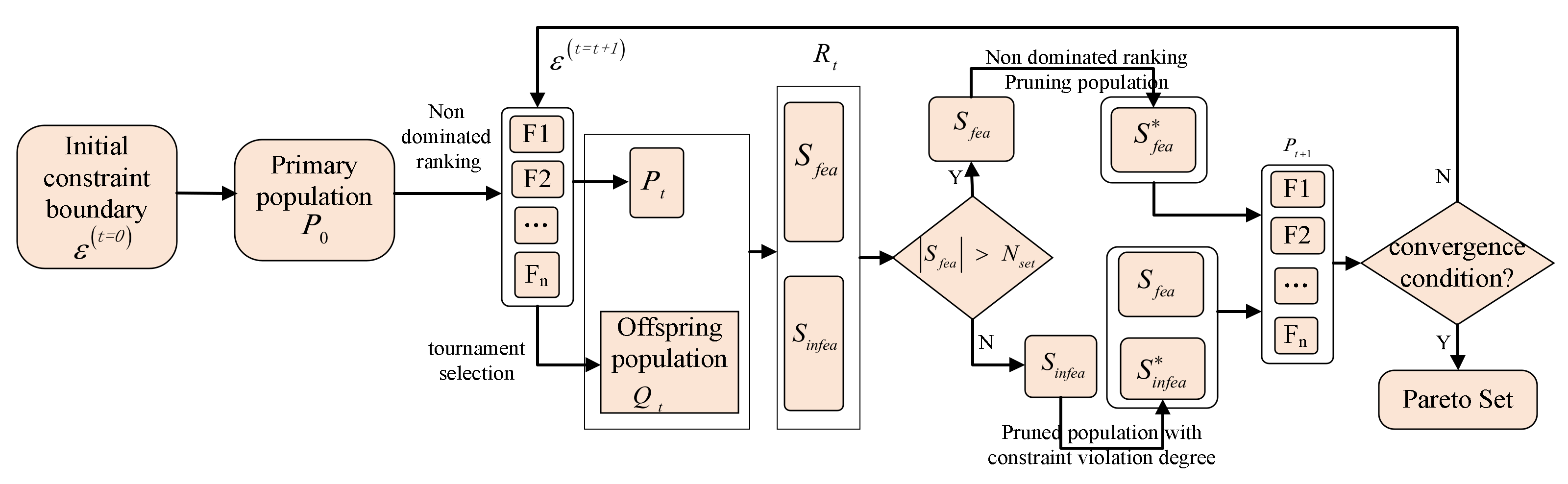
where t is the number of iterations, ${\epsilon }_i^{\left(0\right)}>{\epsilon }_i^{\left(1\right)}>\cdots >{\epsilon }_i^{\left(T\right)}=0$, ${\epsilon }_i^{\left(t\right)}$ decreases gradually with the increase in the number of iterations. The value of $CP$ can usually be taken between two and ten. The greater the $CP$ value, the faster the ${\epsilon }_i^{\left(t\right)}$ value decreases. ${\epsilon }_i^{\left(0\right)}$ is the maximum value of constraint violation degree of all individuals in the population. In this process, it is allowed to retain some infeasible solutions. When ${\epsilon }_i^{\left(T\right)}=0$, it is equivalent to the original constraints to find a better feasible solution. The flow chart of using this mechanism to improve NSGA-III algorithm is shown in Figure 2:

Initialize the constraint boundary ${\epsilon }_{}^{\left(t=0\right)}$ so that all solutions in the population are feasible and randomly generate the initial population ${{\rm P}}_0$ from the search space. In each iteration, the $\epsilon$ constraint boundary will decrease with the increase in generation times. Individuals in the population are divided into several levels (F₁, F₂, …, F_n) according to the dominant relationship between them. In an ideal case, every solution in any state of the population is expected to be within the constraint boundary ${\epsilon }_{}^{\left(t\right)}$, which means that all solutions are $\epsilon$ feasible. Therefore, the multi-objective evolutionary algorithm can focus on balancing the convergence and diversity in the feasible region without considering the initial constraints. However, $\epsilon$ infeasible solutions are inevitable. In order to generate more feasible sub solutions, in the process of generating offspring population $Q_t$, the binary tournament tends to choose $\epsilon$ feasible solutions rather than $\epsilon$ infeasible solutions or tends to choose solutions with small constraint violation degree rather than solutions with large constraint violation degree. In each generation t, the population $R_t$ composed of parent population ${{\rm P}}_t$ and offspring population $Q_t$ is divided into feasible solution set $S_{fea}$ and infeasible solution set $S_{infea}$ according to ${\epsilon }_{}^{\left(t\right)}$. We tend to choose $\epsilon$ feasible solution set $S_{fea}$. Specifically, we have the following two situations:

When $\left|S_{fea}\right|$ is larger than $N$, $N$ solutions are selected from $S_{fea}$ to ${{\rm P}}_{t+1}$ through nondominated sorting and elite selection based on reference points. It consists of two steps: (1) nondominated sorting from feasible set $S_{fea}$, the nondominated solution is selected to approach its Pareto Front; (2) the purpose of elite selection based on reference points is to maintain the diversity of population by providing a group of evenly distributed reference points.

If $\left|S_{fea}\right|<N$, it means that the number of feasible solutions is less than the overall size $N$, then all solutions in $S_{fea}$ are directly added to ${{\rm P}}_{t+1}$. The remaining $\left(N-\left|S_{fea}\right|\right)$ is selected from $S_{infea}$. Here, we rank the solutions in $S_{infea}$ according to the degree of constraint violation, and then add the first $\left(N-\left|S_{fea}\right|\right)$ solutions to ${{\rm P}}_{t+1}$.

So far, it has been obtained to generate a new parent population ${{\rm P}}_{t+1}$ according to the rules of steps 10–14 in Algorithm 1 and continue the next iteration until the maximum number of iterations is reached. At this time, all solutions in the population converge to the original feasible region, and $g_i\left(x\right)\le {\epsilon }_i^{\left(t\right)}$ in Equation (16) becomes $g_i\left(x\right)\le 0$. For the computational complexity, it is equivalent to adding one more target to the algorithm in the process of nondominated sorting. The computational complexity changes $O\left(m{N}^2\right)$ to $O\left(\left(m+1\right)N^2\right)$, $N$ is the number of populations, $m$ is the number of targets, and the constraint strategy itself does not need a lot of computational resources.

5. Results and Discussion

5.1. Comparison of NSGA-II and NSGA-III for Intersection Traffic Signal Timing

NSGA-II and NSGA-III are popular multi-objective genetic algorithms at present. NSGA-II algorithm ensures the population diversity of offspring through crowding operator, while NSGA-III algorithm ensures the population diversity of offspring through reference point operator.

Table 2. Signal cycle length and green time optimized by NSGA-II.

No	The Signal Timing Plans	Delay (s)	Capacity (pcu/h)	Emission (g/h)
1	{68.1658 69.7081 11.9946 16.5632 170.7807}	728,820	4450	10,270
2	{53.1881 12.758 75.4945 29.5342 175.7652}	721,420	4270	10,180
3	{31.5357 51.5544 62.0261 17.2942 165.8719}	714,430	4450	10,090
4	{26.4569 93.7567 48.9091 23.7874 197.2732}	894,530	4400	12,350
5	{14.0952 41.8625 75.4945 29.5342 165.8130}	736,750	4230	10,370
6	{26.2201 66.1706 44.6423 38.6122 180.7325}	825,870	4150	11,490
7	{68.7607 53.9954 11.9199 23.5186 162.2287}	689,010	4330	9780
8	{84.9584 58.7558 18.9508 27.4643 194.4299}	816,070	4350	11,360
9	{30.2102 34.903 68.2779 17.1499 153.7959}	650,660	4430	9300
10	{67.8421 34.448 9.1593 74.7003 189.9675}	855,230	3760	11,850

and

Table 3. Signal cycle length and green time optimized by NSGA-III.

No	The Signal Timing Plans	Delay (s)	Capacity (pcu/h)	Emission (g/h)
1	{39.0975 43.0555 73.5753 10.0621 169.4974}	704,900	4550	9970
2	{36.3100 80.036 35.5746 22.5388 179.1794}	802,310	4370	11,190
3	{11.6566 103.0964 56.8978 21.6485 197.0691}	908,260	4440	12,520
4	{37.0027 79.1176 35.6203 22.5388 178.7817}	798,960	4380	11,150
5	{35.4893 10.4646 114.5714 16.7496 180.5020}	726,930	4490	10,250
6	{44.2563 78.7388 26.0255 22.6166 175.2643}	778,540	4390	10,900
7	{42.2068 22.7983 16.0178 72.4447 157.9363}	732,350	3560	10,320
8	{62.6925 22.5479 37.4215 19.4436 145.564}	588,910	4370	8520
9	{53.3657 12.9113 15.9612 71.0452 157.9234}	713,450	3580	10,080
10	{62.3572 57.5751 46.3018 21.8967 192.4912}	813,620	4420	11,330

respectively show the signal timing plan optimized by the two algorithms and the corresponding delay, traffic capacity and emission values. The first column in Table 2 and Table 3 is the number of solutions, and the second column is the signal timing plan. The corresponding optimization target total delay, capacity and emission values are shown in columns 3–5, respectively. The experiment was completed on an Intel^®® Core™ i5-6500 CPU (3.2 GHz/8 GB RAM) PC with a Windows 7 operating system, and MATLAB R2017a version was used. In the experiment, the number of Pareto solutions obtained in each run was 50 and the number of iterations was 200. The data of 10 solutions and corresponding decision variables were randomly selected for display. Generally, the performance indicators used to measure the performance of these algorithms are divided into four categories [51]. The first is the capacity measure, which calculates the number of nondominated solutions that meet the preset conditions in the optimal solution set. The second is the convergence measure, which measures the distance between the solution in the optimal solution set and the solution in the real PF approximation set. The third is the diversity measure, which measures the distribution of solutions in the optimal solution set. The fourth is the convergence diversity measure, which measures the convergence and diversity of solutions at the same time. In order to avoid the optimization results falling into local optimization due to constraints, the method in this paper adopts the constraint processing strategy. For the traffic signal timing problem to be solved in this paper, we pay more attention to which of NSGA-II and NSGA-III obtains a wider range of traffic efficiency index values. In Table 2 (obtained by NSGA-II), the results show that the delay values range from 650,660 to 894,530, the capacity values 3760 to 4450, and the emission values 9300 to 12,350. In Table 3 (obtained by NSGA-III), the results show that the delay values range from 588,910 to 908,260, the capacity values 3560 to 4550 and the emission values 8520 to 12,520. The range of delay, capacity and emission values optimized by NSGA-III is wider than that optimized by NSGA-II. In order to be more intuitive, Figure 3 shows the three-dimensional diagrams of delay, traffic capacity and emission values from Table 2 and Table 3. In Figure 3, black square (□) is marked as NSGA-II optimized index, and red star (☆) is marked as NSGA-III optimized index, which is connected with black lines. It is easy to see from Figure 3 that the black closed curve surrounds almost all the points marked black square (□). The analysis shows that if combined with the constraint strategy, NSGA-III has more potential to find more appropriate decision variables and obtain the corresponding traffic efficiency indicators.

5.2. Comparison of HCNSGA-III Timing Scheme with Other Methods

Table 4. Signal cycle and green time optimized by HCNSGA-III.

No	The Signal Timing Plans	Delay (s)	Capacity (pcu/h)	Emission (g/h)
1	{10.4776 21.6493 21.6624 18.7874 76.5761}	351,130	3960	5550
2	{28.8036 15.5800 14.7789 13.3130 76.4672}	324,600	4130	5220
3	{34.2579 10.4774 12.1400 18.0794 78.9423}	332,830	4010	5320
4	{28.9858 11.1999 13.4130 11.8399 69.4260}	290,260	4120	4790
5	{10.8266 14.2697 19.6550 27.2291 75.9651}	353,770	3690	5590
6	{15.0242 19.9494 14.4709 16.2260 69.6441}	315,420	3970	5110
7	{31.0451 20.0957 11.2536 27.0959 93.4617}	414,960	3900	6350
8	{29.6870 11.5128 12.2332 19.2062 76.5886}	329,200	3950	5280
9	{20.9733 14.9134 12.9194 16.4478 69.1949}	305,060	3960	4980
10	{10.4312 10.2325 26.7305 27.7060 79.0254}	362,600	3720	5700

shows the signal timing plan and its corresponding traffic efficiency index value obtained by HCNSGA-III algorithm in this paper, which is a representative of Pareto solution. It can be seen from Table 4 that the values of delay, capacity and emission are in the range of [290,260–414,960], [3690–4130] and [4790–5700], respectively. In Figure 3, the blue circle (○) is marked as HCNSGA-III optimized index, which can be more intuitively compared with the optimization value of NSGA-III. Observe the values on the emission coordinate axis and delay coordinate axis in Figure 3, and the value corresponding to HCNSGA-III decreases significantly. Looking at the capacity axis in Figure 3, although there is no significant improvement in the maximum capacity obtained by HCNSGA-III, the number of points close to the maximum capacity is more than that obtained by NSGA-III. We select a solution from Table 4 (the method in this paper) to

Table 5. Signal timing comparison results of the current method, IPSO and HCNSGA-III.

	The Signal Timing Plan	Delay (s)	Capacity (pcu/h)	Emission (g/h)
Current	{34 30 41 36 161}	732,100	4889	12,237
IPSO	{25 20 22 13 100}	454,130	4704	11,848
HCNSGA-III	{29 11 13 12 69}	290,260	4120	4790

. In order to further illustrate the effectiveness of the algorithm, in Table 4, in addition to the results of the actual signal timing scheme, we implemented the improved particle swarm optimization algorithm (IPSO) for this case [34]. By using a difference operator and dynamic relaxation strategy, the diversity of the algorithm is improved, and a better efficiency index value is obtained. Our HCNSGA_III method considers the constraint processing strategy in solving the TST problem to avoid the impact of constraints on the search process. See Table 5 for the comparison with the results of existing signal timing scheme and recent IPSO method. The method in our work significantly reduces vehicle emissions and vehicle delays. Although the total capacity decreases slightly due to the shortening of signal cycle.

6. Conclusions and Future Prospects

Aiming at delay, capacity and emission, this paper studies the multi-objective optimization of intersection signal timing scheme design. The traffic optimization problem has many objectives and is constrained by the traffic environment. The optimization results of signal timing parameters are easy to fall into local optimization. Based on NSGA-III algorithm, by combining multi-objective constraint and $\epsilon$ constraint strategy, this paper verifies the effectiveness of the algorithm through an actual intersection example. By comparing the optimized timing results of NSGA-III and NSGA-II, the advantages of NSGA-III algorithm in traffic signal timing are verified. Compared with the timing results of NSGA-III algorithm, it is verified that the quality of timing results is further improved after the introduction of constraint strategy. In addition, by comparing with the current actual timing scheme and the IPSO optimized timing scheme, the effectiveness of the algorithm is verified, and the optimal/approximately optimal Pareto solution for signal timing is obtained, which improves the traffic efficiency and provides support for the sustainable development of urban traffic.

The limitations of the current research can be considered in future research. Firstly, we should explore the applicability of NSGA-III algorithm improved according to this strategy in network optimization. Secondly, this paper only considers the impact of conventional traffic flow, mixed traffic flow and road vehicle cooperation environment, which can also be considered in upcoming research. Similarly, it is recommended to consider additional traffic efficiency indicators such as queue length. In addition, further research can also focus on the impact of non-maneuvering modes to solve similar optimization problems. In addition, more effective computing technologies should be explored. All these are the direction of our future efforts.

References

- Lei, Y.; Huang, C. Literature review and management expectation on the alleviating urban traffic congestion. China Transp. Rev. 2018, 40, 8–11. [Google Scholar]
- 68% of the World Population Projected to Live in Urban Areas by 2050, Says UN|Department of Economic and Social Affairs. Available online: https://www.un.org/development/desa/en/news/population/2018-revision-of-world-urbanization-prospects.html (accessed on 9 October 2021).
- Wang, Y.; Yang, X.; Liang, H.; Liu, Y. A Review of the Self-Adaptive Traffic Signal Control System Based on Future Traffic Environment. J. Adv. Transp. 2018, 2018 Pt 3, 1096123. [Google Scholar] [CrossRef]
- Chen, G.; Wu, X.; Guo, J.; Meng, J.; Li, C. Global overview for energy use of the world economy: Household-consumption-based accounting based on the world input-output database (WIOD). Energy Econ. 2019, 81, 835–847. [Google Scholar] [CrossRef]
- Beijing Statement of the Second United Nations Global Sustainable Transport Conference, Beijing, China, 14–16 October 2021. Available online: https://www.un.org/sites/un2.un.org/files/gstc2_beijing_statement_16_oct_2021.pdf (accessed on 31 October 2021).
- Liu, S.; Triantis, K.P.; Sarangi, S. A framework for evaluating the dynamic impacts of a congestion pricing policy for a transportation socioeconomic system. Transp. Res. Part A Policy Pract. 2010, 44, 596–608. [Google Scholar] [CrossRef]
- Manual on Uniform Traffic Control Devices for Streets and Highways: MUTCD NPA Webinar Recordings. Available online: https://mutcd.fhwa.dot.gov/mutcd_news.htm#dec_17_20 (accessed on 12 September 2021).
- Chen, P.; Zheng, F.; Lu, G.; Wang, Y. Comparison of Variability of Individual Vehicle Delay and Average Control Delay at Signalized Intersection. Transp. Res. Rec. J. Transp. Res. Board 2016, 2553, 128–137. [Google Scholar] [CrossRef]
- Traffic Signal Timing & Operations Strategies. Available online: https://ops.fhwa.dot.gov/arterial_mgmt/tst_ops.htm (accessed on 18 September 2021).
- Zhao, D.; Dai, Y.; Zhang, Z. Computational intelligence in urban traffic signal control: A survey. IEEE Trans. Syst. Man Cybern. Part C Appl. Rev. 2012, 42, 485–494. [Google Scholar] [CrossRef]
- Qadri, S.; Gke, M.A.; Oner, E. State-of-art review of traffic signal control methods: Challenges and opportunities. Eur. Transp. Res. Rev. 2020, 12, 55. [Google Scholar] [CrossRef]
- Jin, J.; Ma, X.; Kosonen, I. An intelligent control system for traffic lights with simulation-based evaluation. Control. Eng. Pract. 2017, 58, 24–33. [Google Scholar] [CrossRef] [Green Version]
- Vogel, A.; Oremovi, I.; Simi, R.; Ivanjko, E. Improving traffic light control by means of fuzzy logic. In Proceedings of the 60th International Symposium ELMAR-2018, Zadar, Croatia, 16–19 September 2018; pp. 51–56. [Google Scholar] [CrossRef]
- Panovski, D.; Zaharia, T. Simulation-based vehicular traffic lights optimization. In Proceedings of the 2016 12th International Conference on Signal-Image Technology & Internet-Based Systems (SITIS), Naples, Italy, 28 November–1 December 2016; pp. 258–265. [Google Scholar] [CrossRef]
- Hao, W.; Ma, C.X.; Moghimi, B.; Fan, Y.Y.; Gao, Z.B. Robust optimization of signal control parameters for unsaturated intersection based on tabu search-artificial bee colony algorithm. IEEE Access 2018, 6, 32015–32022. [Google Scholar] [CrossRef]
- Elbeltagia, E.; Hegazyb, T.; Griersonb, D. Comparison among five evolutionary-based optimization algorithms. Adv. Eng. Inform. 2005, 19, 43–53. [Google Scholar] [CrossRef]
- Yu, X.; Gen, M. Introduction to Evolutionary Algorithms; Springer: London, UK, 2010; ISBN 978-1-84996-128-8. [Google Scholar]
- Zitzler, E.; Thiele, L.; Laumanns, M.; Fonseca, C.M.; Fonseca, V. Performance assessment of multiobjective optimizers: An analysis and review. IEEE Trans. Evol. Comput. 2003, 7, 117–132. [Google Scholar] [CrossRef] [Green Version]
- Jamal, A.; Rahman, M.T.; Al-Ahmadi, H.M.; Ullah, I.M.; Zahid, M. Intelligent Intersection Control for Delay Optimization: Using Meta-Heuristic Search Algorithms. Sustainability 2020, 12, 1896. [Google Scholar] [CrossRef] [Green Version]
- Mckenney, D.; White, T. Distributed and adaptive traffic signal control within a realistic traffic simulation. Eng. Appl. Artif. Intell. 2013, 26, 574–583. [Google Scholar] [CrossRef]
- Dezani, H.; Marranghello, N.; Damiani, F. Genetic algorithm-based traffic lights timing optimization and routes definition using Petri net model of urban traffic flow. In Proceedings of the 19th World Congress International Federation Automatic Control, Cape Town, South Africa, 24–29 August 2014; pp. 11326–11331. [Google Scholar] [CrossRef] [Green Version]
- Jung, H.; Choi, S.; Park, B.B.; Lee, H.; Son, S.H. Bi-level optimization for eco-traffic signal system. In Proceedings of the International Conference on Connected Vehicles Expo (ICCVE), Seattle, WA, USA, 12–16 September 2016; pp. 29–35. [Google Scholar] [CrossRef]
- Li, X.; Zhao, Z.; Liu, L.; Liu, Y.; Li, P. An optimization model of multi-intersection signal control for trunk road under collaborative information. J. Control. Sci. Eng. 2017, 2017, 2846987. [Google Scholar] [CrossRef] [Green Version]
- Clerc, M.; Kennedy, J. The particle swarm—Explosion, stability, and convergence in a multidimensional complex space. IEEE Trans. Evol. Comput. 2002, 6, 58–73. [Google Scholar] [CrossRef] [Green Version]
- García-Nieto, J.; Alba, E.; Carolina Olivera, A. Swarm intelligence for traffic light scheduling: Application to real urban areas. Eng. Appl. Artif. Intell. 2012, 25, 274–283. [Google Scholar] [CrossRef]
- Garcia-Nieto, J.; Olivera, A.C.; Alba, E. Optimal cycle program of traffic lights with particle swarm optimization. IEEE Trans. Evol. Comput. 2013, 17, 823–839. [Google Scholar] [CrossRef] [Green Version]
- Kou, W.; Chen, X.; Yu, L.; Gong, H. Multiobjective optimization model of intersection signal timing considering emissions based on field data: A case study of Beijing. J. Air Waste Manag. Assoc. 2018, 68, 836–848. [Google Scholar] [CrossRef] [Green Version]
- Baskan, O. A multiobjective bilevel programming model for environmentally friendly traffic signal timings. Adv. Civ. Eng. 2019, 2019, 1638618. [Google Scholar] [CrossRef] [Green Version]
- Pholdee, N.; Bureerat, S. Comparative performance of meta-heuristic algorithms for mass minimization of trusses with dynamic constraints. Adv. Eng. Softw. 2014, 75, 1–13. [Google Scholar] [CrossRef]
- Deb, K.; Pratap, A.; Agarwal, S.; Meyarivan, T. A fast and elitist multiobjective genetic algorithm: NSGA-II. IEEE Trans. Evol. Comput. 2002, 6, 182–197. [Google Scholar] [CrossRef] [Green Version]
- Sun, D.; Benekohal, R.F.; Waller, S.T. Multiobjective traffic signal timing optimization using non-dominated sorting genetic algorithm. In Proceedings of the IEEE Intelligent Vehicles Symposium, Columbus, OH, USA, 9–11 June 2003; pp. 198–203. [Google Scholar] [CrossRef]
- Park, B.; Messer, C.; Urbanik, T., II. Traffic signal optimization program for oversaturated conditions: Genetic algorithm approach. Transp. Res. Rec. 1999, 1683, 133–142. [Google Scholar] [CrossRef]
- Li, Y.; Yu, L.; Tao, S.; Chen, K. Multi-objective optimization of traffic signal timing for oversaturated intersection. Math. Probl. Eng. 2013, 2013, 182643. [Google Scholar] [CrossRef]
- Jia, H.; Lin, Y.; Luo, Q.; Li, Y.; Miao, H. Multi-objective optimization of urban road intersection signal timing based on particle swarm optimization algorithm. Adv. Mech. Eng. 2019, 11, 1687814019842498. [Google Scholar] [CrossRef] [Green Version]
- Bechikh, S.; Elarbi, M.; Said, L.B. Many-objective Optimization Using Evolutionary Algorithms: A Survey. In Recent Advances in Evolutionary Multi-Objective Optimization, 1st ed.; Bechikh, S., Datta, R., Gupta, A., Eds.; Springer International Publishing: Cham, Switzerland, 2017; Volume 20, pp. 105–137. Available online: https://www.springer.com/gp/book/9783319429779 (accessed on 1 May 2019).
- Deb, K.; Jain, H. An Evolutionary Many-Objective Optimization Algorithm Using Reference-Point-Based Nondominated Sorting Approach, Part I: Solving Problems with Box Constraints. IEEE Trans. Evol. Comput. 2014, 18, 577–601. [Google Scholar] [CrossRef]
- Michalewicz, Z.; Schoenauer, M. Evolutionary algorithm for constrained parameter optimization problems. Evol. Comput. 1996, 4, 1–32. [Google Scholar] [CrossRef]
- Coello, C.A.C. Theoretical and numerical constraint-handling techniques used with evolutionary algorithms: A survey of the state of the art. Comput. Methods Appl. Mech. Eng. 2002, 191, 1245–1287. [Google Scholar] [CrossRef]
- Mezura-Montes, E.; Coello, C.A.C. Constraint-Handling in nature-inspired numerical optimization: Past, present and future. Swarm Evol. Comput. 2011, 1, 173–194. [Google Scholar] [CrossRef]
- Zeng, S.; Jiao, R.; Li, C.; Wang, R. Constrained optimization by solving equivalent dynamic loosely-constrained multiobjective optimization problem. Int. J. Bio-Inspired Comput. 2019, 13, 86–101. [Google Scholar] [CrossRef]
- Zeng, S.; Jiao, R.; Li, C.; Li, X.; Alkasassbeh, J.S. A general framework of dynamic constrained multiobjective evolutionary algorithms for constrained optimization. IEEE Trans. Cybern. 2017, 47, 2678–2688. [Google Scholar] [CrossRef]
- Akcxelik, R.; Rouphail, N.M. Estimation of delays at traffic signals for variable demand conditions. Transp. Res. B Meth. 1993, 27, 109–131. [Google Scholar] [CrossRef]
- Shafabakhsh, G.; Taghizadeh, S.A.; Kooshki, S.M. Investigation and sensitivity analysis of air pollution caused by road transportation at signalized intersections using IVE model in Iran. Eur. Transp. Res. Rev. 2018, 10, 7. [Google Scholar] [CrossRef] [Green Version]
- Ding, S.; Chen, X.; Yu, L.; Wang, X. Arterial Offset Optimization Considering the Delay and Emission of Platoon: A Case Study in Beijing. Sustainability 2019, 11, 3882. [Google Scholar] [CrossRef] [Green Version]
- Kodjak, D. Policies to Reduce Fuel Consumption, Air Pollution, and Carbon Emissions from Vehicles in G20 Nations. International Council on Clean Transportation. Available online: http://www.indiaenvironmentportal.org.in/content/412517/policies-to-reduce-fuel-consumption-air-pollution-and-carbon-emissions-from-vehicles-in-g20-nations/ (accessed on 8 May 2020).
- Shaheen, S.A.; Lipman, T.E. Reducing greenhouse emissions and fuel consumption. IATSS Res. 2007, 31, 6–20. [Google Scholar] [CrossRef] [Green Version]
- Liao, T.Y. A fuel-based signal optimization model. Transp. Res. Part D Transp. Environ. 2013, 23, 1–8. [Google Scholar] [CrossRef]
- Kwak, J.; Park, B.; Lee, J. Evaluating the impacts of urban corridor traffic signal optimization on vehicle emissions and fuel consumption. Transp. Plan Technol. 2012, 35, 145–160. [Google Scholar] [CrossRef]
- Das, I.; Dennis, J.E. Normal-boundary intersection: A new method for generating the pareto surface in nonlinear multicriteria optimization problems. SIAM J. Optim. 1998, 8, 631–657. [Google Scholar] [CrossRef] [Green Version]
- Rj, A.; Sz, A.; Clb, C. A feasible-ratio control technique for constrained optimization. Inf. Sci. 2019, 502, 201–217. [Google Scholar] [CrossRef]
- Jiang, S.; Ong, Y.; Zhang, J.; Feng, L. Consistencies and contradictions of performance metrics in multiobjective optimization. IEEE Trans. Cybern. 2014, 44, 2391–2404. [Google Scholar] [CrossRef]
Figure 1.
Sequence of four signal stages and its traffic flow diagram.
Figure 2.
Flow chart of NSGA-III with hybrid constraint mechanism.
Figure 3.
Comparison of traffic capacity, delay and emission values optimized by NSGA-II, NSGA-III and HCNSGA-III.