
Study of Spatiotemporal Changes and Driving Factors of Habitat Quality: A Case Study of the Agro-Pastoral Ecotone in Northern Shaanxi, China

 ,
,
Abstract
:1. Introduction
2. Materials and Methods
2.1. Study Area
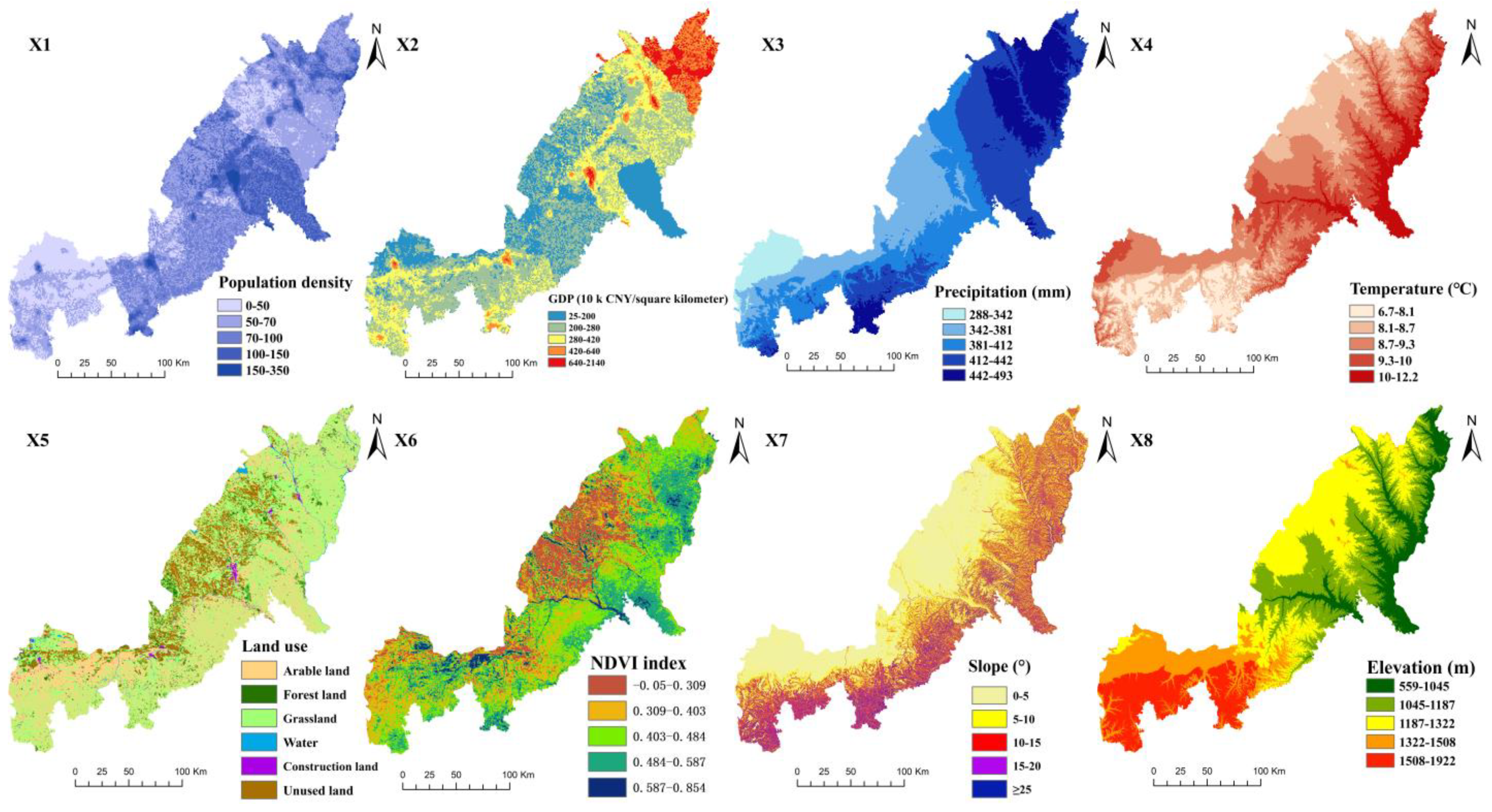
2.2. Data Source
2.3. Methods
2.3.1. Analysis of the Landscape Pattern Index
2.3.2. Assessment of Habitat Quality
2.3.3. Global Moran’s I
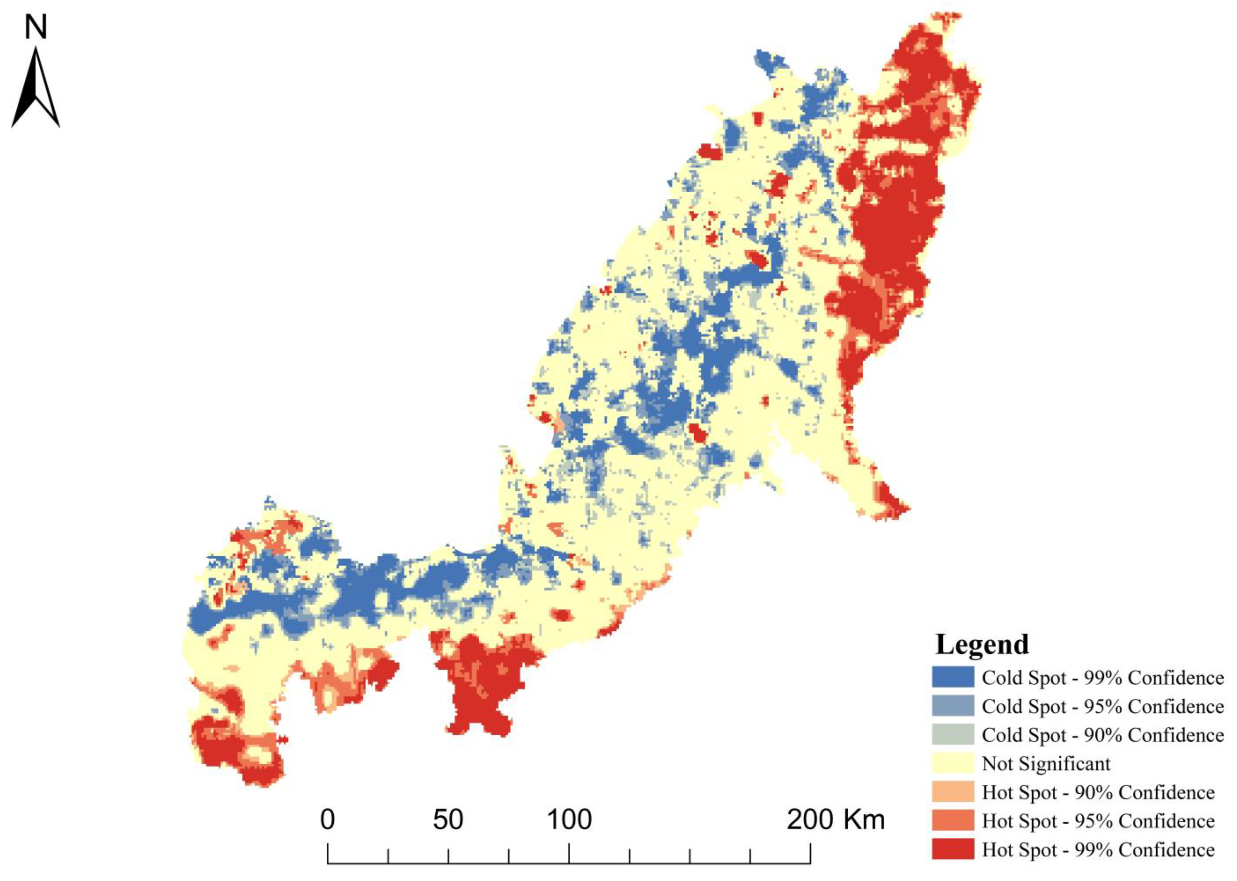
2.3.4. Hot-Spot Analysis (Getis-Ord Gi*)
2.3.5. Geo-Detector
3. Results
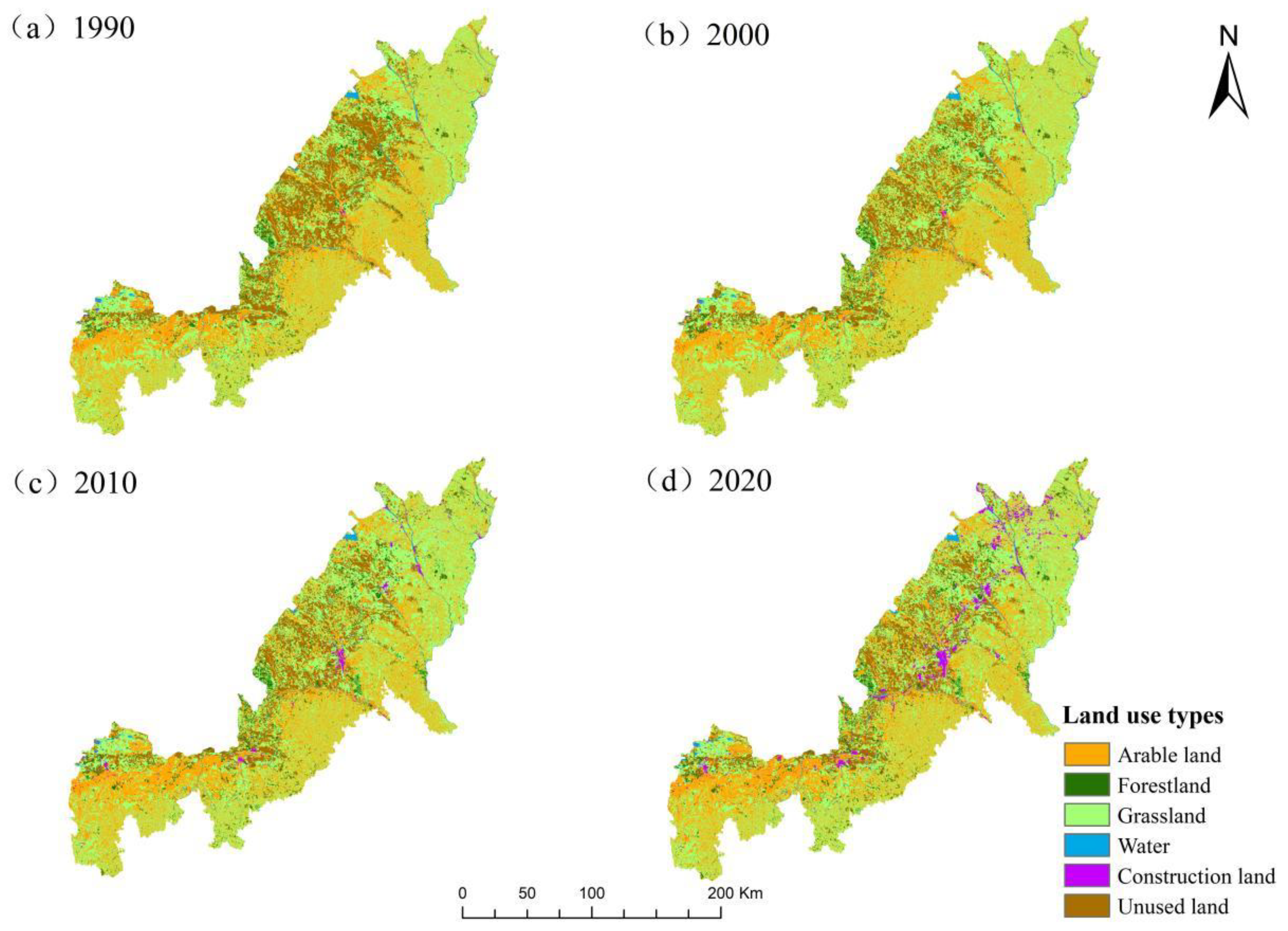
3.1. Land-Use Change in the Agro-Pastoral Ecotone of Northern Shaanxi
3.2. Analysis of Landscape Pattern Index in the Agro-Pastoral Ecotone of Northern Shaanxi
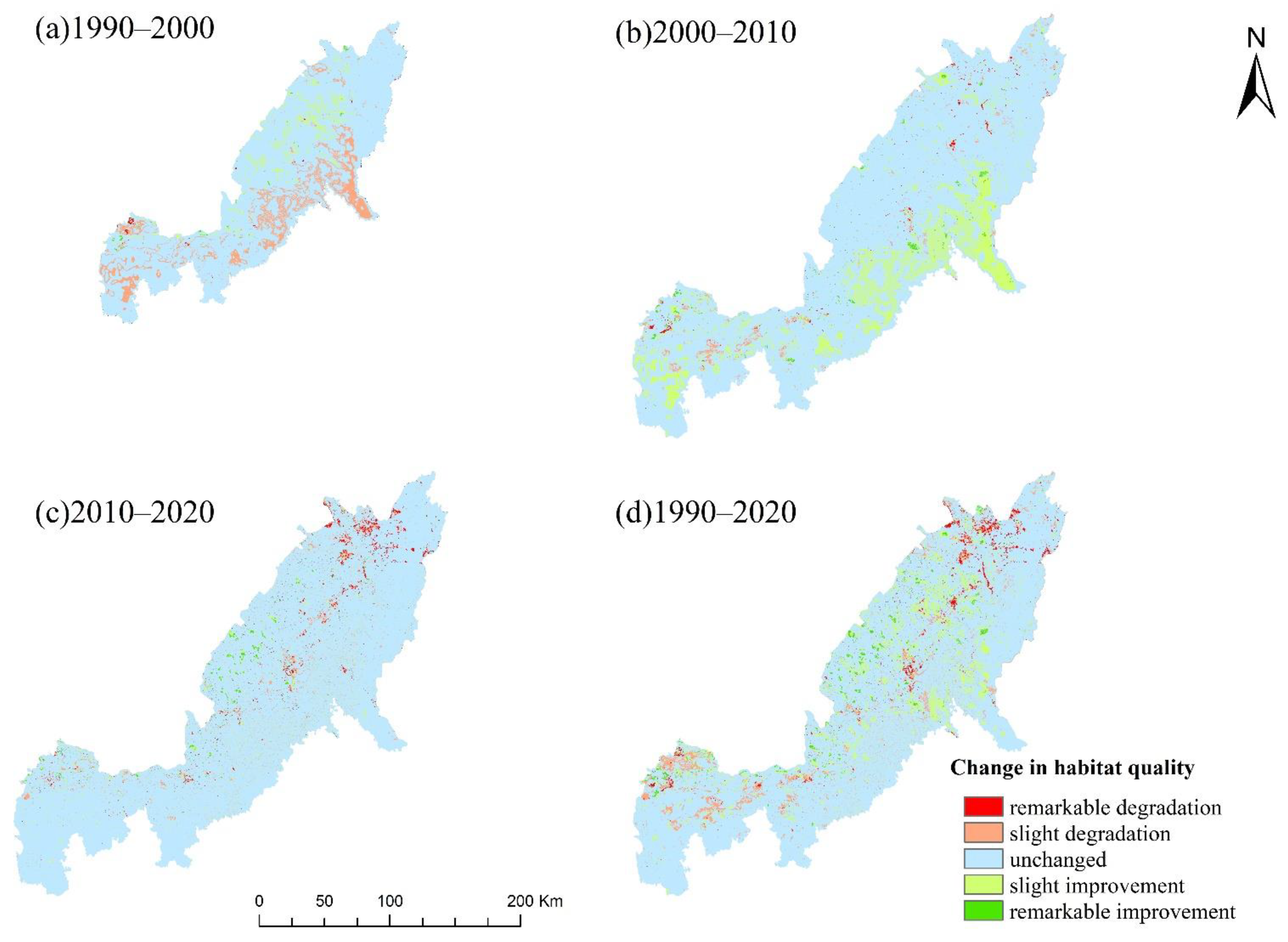
3.3. Spatiotemporal Change in Habitat Quality
3.4. Changes in Habitat Quality Characteristics of Different Land Types
3.5. Analysis of the Driving Force of Habitat Quality Changes Based on the Geo-Detector
4. Discussion
4.1. The Relationship of Land-Use Change and Habitat Quality
4.2. Driving Factors of Habitat Quality
4.3. Implication for Habitat-Quality Conservation
4.4. Limitations and Prospective
5. Conclusions
Author Contributions
Funding
Institutional Review Board Statement
Informed Consent Statement
Data Availability Statement
Acknowledgments
Conflicts of Interest
References
- Costanza, R.; D’Arge, R.; de Groot, R.; Farber, S.; Grasso, M.; Hannon, B.; Limburg, K.; Naeem, S.; O’Neill, R.V.; Paruelo, J.; et al. The value of the world’s ecosystem services and natural capital. Nature 1997, 387, 253–260. [Google Scholar] [CrossRef]
- Moreira, M.; Fonseca, C.; Vergílio, M.; Calado, H.; Gil, A. Spatial assessment of habitat conservation status in a Macaronesian island based on the InVEST model: A case study of Pico Island (Azores, Portugal). Land Use Policy 2018, 78, 637–649. [Google Scholar] [CrossRef]
- Di Febbraro, M.; Sallustio, L.; Vizzarri, M.; De Rosa, D.; De Lisio, L.; Loy, A.; Eichelberger, B.A.; Marchetti, M. Expert-based and correlative models to map habitat quality: Which gives better support to conservation planning? Glob. Ecol. Conserv. 2018, 16, e513. [Google Scholar] [CrossRef]
- Tang, L.; Ke, X.; Chen, Y.; Wang, L.; Zhou, Q.; Zheng, W.; Xiao, B. Which impacts more seriously on natural habitat loss and degradation? Cropland expansion or urban expansion? Land Degrad. Dev. 2021, 32, 946–964. [Google Scholar] [CrossRef]
- Sun, X.; Jiang, Z.; Liu, F.; Zhang, D. Monitoring spatial-temporal dynamics of habitat quality in Nansihu Lake basin, eastern China, from 1980 to 2015. Ecol. Indic. 2019, 102, 716–723. [Google Scholar] [CrossRef]
- Caro, C.; Marques, J.C.; Cunha, P.P.; Teixeira, Z. Ecosystem services as a resilience descriptor in habitat risk assessment using the InVEST model. Ecol. Indic. 2020, 115, 106426. [Google Scholar] [CrossRef]
- Yang, H.; Huang, Q.; Zhang, J.; Songer, M.; Liu, J. Range-wide assessment of the impact of China’s nature reserves on giant panda habitat quality. Sci. Total Environ. 2021, 769, 145081. [Google Scholar] [CrossRef]
- Wynne, S.P.; Côté, I.M. Effects of habitat quality and fishing on Caribbean spotted spiny lobster populations. J. Appl. Ecol. 2007, 44, 488–494. [Google Scholar] [CrossRef]
- Zhu, Z.; Huai, W.; Yang, Z.; Li, D.; Wang, Y. Assessing habitat suitability and habitat fragmentation for endangered Siberian cranes in Poyang Lake region, China. Ecol. Indic. 2021, 125, 107594. [Google Scholar] [CrossRef]
- Brown, G.; Brabyn, L. The extrapolation of social landscape values to a national level in New Zealand using landscape character classification. Appl. Geogr. 2012, 35, 84–94. [Google Scholar] [CrossRef]
- Bai, L.; Xiu, C.; Feng, X.; Liu, D. Influence of urbanization on regional habitat quality: A case study of Changchun City. Habitat Int. 2019, 93, 102042. [Google Scholar] [CrossRef]
- Zhang, X.; Zhou, J.; Li, G.; Chen, C.; Li, M.; Luo, J. Spatial pattern reconstruction of regional habitat quality based on the simulation of land use changes from 1975 to 2010. J. Geogr. Sci. 2020, 30, 601–620. [Google Scholar] [CrossRef]
- Li, M.; Zhou, Y.; Xiao, P.; Tian, Y.; Huang, H.; Xiao, L. Evolution of Habitat Quality and Its Topographic Gradient Effect in Northwest Hubei Province from 2000 to 2020 Based on the InVEST Model. Land 2021, 10, 857. [Google Scholar] [CrossRef]
- Wang, Y.; Dai, E. Spatial-temporal changes in ecosystem services and the trade-off relationship in mountain regions: A case study of Hengduan Mountain region in Southwest China. J. Clean. Prod. 2020, 264, 121573. [Google Scholar] [CrossRef]
- Yang, Y. Evolution of habitat quality and association with land-use changes in mountainous areas: A case study of the Taihang Mountains in Hebei Province, China. Ecol. Indic. 2021, 129, 107967. [Google Scholar] [CrossRef]
- Yohannes, H.; Soromessa, T.; Argaw, M.; Dewan, A. Spatio-temporal changes in habitat quality and linkage with landscape characteristics in the Beressa watershed, Blue Nile basin of Ethiopian highlands. J. Environ. Manag. 2021, 281, 111885. [Google Scholar] [CrossRef]
- Upadhaya, S.; Dwivedi, P. Conversion of forestlands to blueberries: Assessing implications for habitat quality in Alabaha river watershed in Southeastern Georgia, United States. Land Use Policy 2019, 89, 104229. [Google Scholar] [CrossRef]
- Zhu, C.; Zhang, X.; Zhou, M.; He, S.; Gan, M.; Yang, L.; Wang, K. Impacts of urbanization and landscape pattern on habitat quality using OLS and GWR models in Hangzhou, China. Ecol. Indic. 2020, 117, 106654. [Google Scholar] [CrossRef]
- Li, Y.; Liu, W.; Feng, Q.; Zhu, M.; Yang, L.; Zhang, J. Quantitative Assessment for the Spatiotemporal Changes of Ecosystem Services, Tradeoff–Synergy Relationships and Drivers in the Semi-Arid Regions of China. Remote Sens. 2022, 14, 239. [Google Scholar] [CrossRef]
- Fu, B.J.; Stafford-Smith, M.; Wang, Y.F.; Wu, B.F.; Yu, X.B.; Lv, N.; Ojima, D.S.; Lv, Y.H.; Fu, C.; Liu, Y.; et al. The Global-DEP conceptual framework—Research on dryland ecosystems to promote sustainability. Curr. Opin. Environ. Sust. 2021, 48, 17–28. [Google Scholar] [CrossRef]
- Peng, Y.; Fu, B.J.; Zhang, L.X.; Yu, X.B.; Fu, C.; Diop, S.; Hirwa, H.; Guisse, A.; Li, F.D. Global Dryland Ecosystem Programme (G-DEP): Africa consultative meeting report. J. Arid Land 2020, 12, 538–544. [Google Scholar] [CrossRef]
- Feng, X.M.; Stafford-Smith, M.; Zhang, L.; Lyu, N.; Lyu, Y.H.; Fu, B.J.; Xu, Z.H. Global Dryland Ecosystem Programme (Global-DEP): Australasian consultation report. J. Soil. Sediment. 2020, 20, 1807–1810. [Google Scholar] [CrossRef] [Green Version]
- Wang, Y.; Dong, Y.; Su, Z.; Mudd, S.M.; Zheng, Q.; Hu, G.; Yan, D. Spatial distribution of water and wind erosion and their influence on the soil quality at the agropastoral ecotone of North China. Int. Soil Water Conserv. Res. 2020, 8, 253–265. [Google Scholar] [CrossRef]
- Pei, H.; Liu, M.; Jia, Y.; Zhang, H.; Li, Y.; Xiao, Y. The trend of vegetation greening and its drivers in the Agro-pastoral ecotone of northern China, 2000–2020. Ecol. Indic. 2021, 129, 108004. [Google Scholar] [CrossRef]
- Yang, Y.; Wang, K.; Liu, D.; Zhao, X.; Fan, J. Effects of land-use conversions on the ecosystem services in the agro-pastoral ecotone of northern China. J. Clean. Prod. 2020, 249, 119360. [Google Scholar] [CrossRef]
- Qi, Y.; Chang, Q.; Jia, K.; Liu, M.; Liu, J.; Chen, T. Temporal-spatial variability of desertification in an agro-pastoral transitional zone of northern Shaanxi Province, China. Catena 2012, 88, 37–45. [Google Scholar] [CrossRef]
- Shehab, Z.N.; Jamil, N.R.; Aris, A.Z.; Shafie, N.S. Spatial variation impact of landscape patterns and land use on water quality across an urbanized watershed in Bentong, Malaysia. Ecol. Indic. 2021, 122, 107254. [Google Scholar] [CrossRef]
- Chiang, L.; Lin, Y.; Huang, T.; Schmeller, D.S.; Verburg, P.H.; Liu, Y.; Ding, T. Simulation of ecosystem service responses to multiple disturbances from an earthquake and several typhoons. Landsc. Urban Plan. 2014, 122, 41–55. [Google Scholar] [CrossRef]
- Sharp, R.; Douglass, J.; Wolny, S.; Arkema, K.; Bernhardt, J.; Bierbower, W.; Chaumont, N.; Denu, D.; Fisher, D.; Glowinski, K.; et al. InVEST 3.8.7. User’s Guide; Collaborative Publication by the Natural Capital Project, Stanford University, University of Minnesota, the Nature Conservancy, World Wildlife Fund; Stanford University: Stanford, CA, USA, 2020. [Google Scholar]
- Li, Y.; Duo, L.; Zhang, M.; Wu, Z.; Guan, Y. Assessment and Estimation of the Spatial and Temporal Evolution of Landscape Patterns and Their Impact on Habitat Quality in Nanchang, China. Land 2021, 10, 1073. [Google Scholar] [CrossRef]
- Yang, Z.; Wang, S.; Guo, M.; Tian, J.; Zhang, Y. Spatiotemporal Differentiation of Territorial Space Development Intensity and Its Habitat Quality Response in Northeast China. Land 2021, 10, 573. [Google Scholar] [CrossRef]
- Khosravi Mashizi, A.; Escobedo, F.J. Socio-ecological assessment of threats to semi-arid rangeland habitat in Iran using spatial models and actor group opinions. J. Arid Environ. 2020, 177, 104136. [Google Scholar] [CrossRef]
- Raji, S.A.; Odunuga, S.; Fasona, M. Quantifying ecosystem service interactions to support environmental restoration in a tropical semi-arid basin. Acta Geophys. 2021, 69, 1813–1841. [Google Scholar] [CrossRef]
- Fan, X.; Gu, X.; Yu, H.; Long, A.; Tiando, D.S.; Ou, S.; Li, J.; Rong, Y.; Tang, G.; Zheng, Y.; et al. The Spatial and Temporal Evolution and Drivers of Habitat Quality in the Hung River Valley. Land 2021, 10, 1369. [Google Scholar] [CrossRef]
- Liu, C.; Wang, C. Spatio-temporal evolution characteristics of habitat quality in the Loess Hilly Region based on land use change: A case study in Yuzhong County. Acta Ecol. Sin. 2018, 38, 7300–7311. (In Chinese) [Google Scholar]
- Wang, J.; Xu, C. Geodetectors: Principles and prospective. Acta Geogr. Sin. 2017, 72, 116–134. (In Chinese) [Google Scholar]
- Chen, M.; Bai, Z.; Wang, Q.; Shi, Z. Habitat Quality Effect and Driving Mechanism of Land Use Transitions: A Case Study of Henan Water Source Area of the Middle Route of the South-to-North Water Transfer Project. Land 2021, 10, 796. [Google Scholar] [CrossRef]
- Wan, H.W.; Li, H.X.; Wu, J.H.; Liu, Y.P. Spatial distribution pattern in mammal and bird richness and their relationship with ecosystem services in Sanjiangyuan National Park, China. J. Mt. Sci.-Engl. 2021, 18, 1662–1677. [Google Scholar] [CrossRef]
- Liu, Q.; Yang, Z.; Han, F.; Shi, H.; Wang, Z.; Chen, X. Ecological Environment Assessment in World Natural Heritage Site Based on Remote-Sensing Data. A Case Study from the Bayinbuluke. Sustainability 2019, 11, 6385. [Google Scholar] [CrossRef] [Green Version]
- Xu, J.; Liu, S.; Zhao, S.; Wu, X.; Hou, X.; An, Y.; Shen, Z. Spatiotemporal Dynamics of Water Yield Service and Its Response to Urbanisation in the Beiyun River Basin, Beijing. Sustainability 2019, 11, 4361. [Google Scholar] [CrossRef] [Green Version]
- Yuan, X.; Shao, Y.; Li, Y.; Liu, Y.; Wang, Y.; Wei, X.; Wang, X.; Zhao, Y. Cultivated land quality improvement to promote revitalization of sandy rural areas along the Great Wall in northern Shaanxi Province, China. J. Rur. Stud. 2019; in press. [Google Scholar] [CrossRef]
- Yang, J.; Xie, B.; Zhang, D.G. Spatial-temporal evolution of habitat quality and its influencing factors in the Yellow River Basin based on InVEST model and GeoDetector. J. Desert Res. 2021, 41, 12–22. (In Chinese) [Google Scholar]
- Zhang, X.; Song, W.; Lang, Y.; Feng, X.; Yuan, Q.; Wang, J. Land use changes in the coastal zone of China’s Hebei Province and the corresponding impacts on habitat quality. Land Use Policy 2020, 99, 104957. [Google Scholar] [CrossRef]
- He, J.; Huang, J.; Li, C. The evaluation for the impact of land use change on habitat quality: A joint contribution of cellular automata scenario simulation and habitat quality assessment model. Ecol. Model. 2017, 366, 58–67. [Google Scholar] [CrossRef]
- Burel, F.; Baudry, J. Habitat quality and connectivity in agricultural landscapes: The role of land use systems at various scales in time. Ecol. Indic. 2005, 5, 305–313. [Google Scholar] [CrossRef]
- Dutta, S.; Jhala, Y. Planning agriculture based on landuse responses of threatened semiarid grassland species in India. Biol. Conserv. 2014, 175, 129–139. [Google Scholar] [CrossRef]
- Zhang, X.; Lyu, C.; Fan, X.; Bi, R.; Xia, L.; Xu, C.; Sun, B.; Li, T.; Jiang, C. Spatiotemporal Variation and Influence Factors of Habitat Quality in Loess Hilly and Gully Area of Yellow River Basin: A Case Study of Liulin County, China. Land 2022, 11, 127. [Google Scholar] [CrossRef]
- Berta Aneseyee, A.; Noszczyk, T.; Soromessa, T.; Elias, E. The InVEST Habitat Quality Model Associated with Land Use/Cover Changes: A Qualitative Case Study of the Winike Watershed in the Omo-Gibe Basin, Southwest Ethiopia. Remote Sens. 2020, 12, 1103. [Google Scholar] [CrossRef] [Green Version]
- Han, X.; Lv, P.; Zhao, S.; Sun, Y.; Yan, S.; Wang, M.; Han, X.; Wang, X. The Effect of the Gully Land Consolidation Project on Soil Erosion and Crop Production on a Typical Watershed in the Loess Plateau. Land 2018, 7, 113. [Google Scholar] [CrossRef] [Green Version]
- Rasool, M.A.; Hassan, M.A.; Zhang, X.; Zeng, Q.; Jia, Y.; Wen, L.; Lei, G. Habitat Quality and Social Behavioral Association Network in a Wintering Waterbirds Community. Sustainability 2021, 13, 6044. [Google Scholar] [CrossRef]
- Heredia-R, M.; Torres, B.; Cabrera-Torres, F.; Torres, E.; Díaz-Ambrona, C.G.H.; Pappalardo, S.E. Land Use and Land Cover Changes in the Diversity and Life Zone for Uncontacted Indigenous People: Deforestation Hotspots in the Yasuní Biosphere Reserve, Ecuadorian Amazon. Forests 2021, 12, 1539. [Google Scholar] [CrossRef]
- Zhang, Y.-Z.; Jiang, Z.-Y.; Li, Y.-Y.; Yang, Z.-G.; Wang, X.-H.; Li, X.-B. Construction and Optimization of an Urban Ecological Security Pattern Based on Habitat Quality Assessment and the Minimum Cumulative Resistance Model in Shenzhen City, China. Forests 2021, 12, 847. [Google Scholar] [CrossRef]
- Su, X.; Zhou, Y.; Li, Q. Designing Ecological Security Patterns Based on the Framework of Ecological Quality and Ecological Sensitivity: A Case Study of Jianghan Plain, China. Int. J. Environ. Res. Public Health 2021, 18, 8383. [Google Scholar] [CrossRef] [PubMed]
- Zhao, Y.; Liu, L.; Kang, S.; Ao, Y.; Han, L.; Ma, C. Quantitative Analysis of Factors Influencing Spatial Distribution of Soil Erosion Based on Geo-Detector Model under Diverse Geomorphological Types. Land 2021, 10, 604. [Google Scholar] [CrossRef]


| Primary Land-Use Type | Secondary Land-Use Type |
|---|---|
| Arable land | Paddy field, Dry land |
| Forestland | Forest, Shrub, Sparse Forest, Other forest |
| Grassland | High-coverage grassland, Moderate-coverage grassland, Low-coverage grassland |
| Water | River/Canal, Lake, Reservoir/Pond, Mudflat, Wetland |
| Construction land | Urban, Residents, Other construction |
| Unused land | Sand land, Salinity land, Bare land |
| Metric | Acronym | Scale | Description |
|---|---|---|---|
| Patch Density | PD | Class/ Landscape | This index represents the number of patches per 100 ha. It reflects the degree of fragmentation of the landscape. The larger that the PD value is, the more fragmented that the landscape is. |
| Mean of Patch Area | AREA_MN | Class/ Landscape | This index indicates the extent of landscape fragmentation. The smaller that the value is, the more broken that it is. |
| Edge Density, | ED | Class/ Landscape | Edge density includes both landscape edge density and the type of edge density. Landscape edge density refers to the edge length between landscape patches per unit of area within the landscape range. The type of edge density refers to the edge length of a type of landscape patch with an adjacent patch. |
| Largest Patch Index | LPI | Class/ Landscape | The Largest Patch Index is used to determine the dominant patch type in the landscape. |
| Landscape Shape Index | LSI | Class/ Landscape | Landscape Shape Index indicates the shape index of patches in a landscape pattern. |
| Area-Weighted Mean Fractal Dimension Index | FRAC_AM | Class/ Landscape | This index reflects the degree of irregularity and fragmentation of the landscape type. The more irregular that the shape of the landscape is, the higher that the value of the fractal dimension is. Values range from 1 to 2, and values closer to 1 indicate areas of relatively simple shapes, such as a square or a circle. Values close to 2 indicate both complex and irregular shapes. |
| Shannon’s Diversity Index | SHDI | Class/ Landscape | This index can reflect landscape heterogeneity and is particularly sensitive to uneven distributions of different patchwork types in a landscape. SHDI is also a sensitive indicator when comparing and analyzing the diversity and heterogeneity of different landscapes or of the same landscape in different periods. |
| Shannon’s Evenness Index | SHEI | Class/ Landscape | SHEI equals the Shannon Diversity Index divided by the maximum possible diversity at a given landscape abundance (equal distribution across patch types). |
| Interspersion and Juxtaposition Index | IJI | Class/ Landscape | IJI is one of the most important indicators to describe the spatial pattern of a landscape. IJI has a significant response to the distribution of characteristics of ecosystems that are severely constrained by certain natural conditions. |
| Contagion Index, | CONTAG | Landscape | This index describes the degree of non-randomness or clustering of different patch types in the landscape. High values indicate good connectivity of a dominant patch type in the landscape; low values indicate a dense pattern with multiple elements and a high degree of landscape fragmentation. |
| Aggregation Index | AI | Class/ Landscape | AI represents connectivity between patches of each landscape type. |
| Threat Source | Weight | Maximum Impact Distance (Km) | Decay Type |
|---|---|---|---|
| Arable land | 0.6 | 3 | linear |
| Urban | 1 | 10 | exponential |
| Residents | 0.7 | 2 | exponential |
| Other construction land | 0.5 | 1 | exponential |
| Highway | 0.6 | 3 | linear |
| National road | 0.6 | 3 | linear |
| Provincial road | 0.5 | 2 | linear |
| County road | 0.4 | 1 | linear |
| Railway | 1 | 5 | linear |
| Land-Use Type | Habitat Suitability | Threats | |||||||||
|---|---|---|---|---|---|---|---|---|---|---|---|
| Primary Land-Use Types | Secondary Land-Use Type | Arable Land | Urban | Rural Residents | Construction Land | Highway | National Road | Provincial Road | County Road | Rail-Way | |
| Arable Land | Paddy field | 0.5 | 0.3 | 0.4 | 0.3 | 0.4 | 0.7 | 0.6 | 0.4 | 0.3 | 0.7 |
| Dry land | 0.5 | 0.3 | 0.4 | 0.3 | 0.4 | 0.7 | 0.6 | 0.4 | 0.3 | 0.7 | |
| Forestland | Woodland | 1 | 0.5 | 0.8 | 0.7 | 0.8 | 0.7 | 0.6 | 0.5 | 0.4 | 0.8 |
| Shrub | 0.8 | 0.5 | 0.7 | 0.6 | 0.7 | 0.7 | 0.6 | 0.5 | 0.4 | 0.8 | |
| Sparse forest | 0.5 | 0.4 | 0.5 | 0.4 | 0.55 | 0.7 | 0.6 | 0.5 | 0.4 | 0.8 | |
| Other forest | 0.3 | 0.2 | 0.2 | 0.2 | 0.45 | 0.7 | 0.6 | 0.5 | 0.4 | 0.8 | |
| Grassland | High-coverage grassland | 0.8 | 0.4 | 0.65 | 0.6 | 0.75 | 0.5 | 0.4 | 0.3 | 0.2 | 0.55 |
| Moderate-coverage grassland | 0.5 | 0.3 | 0.55 | 0.5 | 0.6 | 0.5 | 0.4 | 0.3 | 0.2 | 0.55 | |
| Low-coverage grassland | 0.3 | 0.2 | 0.5 | 0.4 | 0.55 | 0.5 | 0.4 | 0.3 | 0.2 | 0.55 | |
| Water | River | 0.8 | 0.65 | 0.8 | 0.7 | 0.9 | 0.65 | 0.6 | 0.5 | 0.3 | 0.7 |
| Lake | 0.9 | 0.65 | 0.8 | 0.7 | 0.9 | 0.65 | 0.6 | 0.5 | 0.3 | 0.7 | |
| Pond | 0.8 | 0.65 | 0.8 | 0.7 | 0.9 | 0.65 | 0.6 | 0.5 | 0.3 | 0.7 | |
| Beach | 0.5 | 0.2 | 0.3 | 0.2 | 0.3 | 0.65 | 0.6 | 0.5 | 0.3 | 0.7 | |
| Marsh | 0.9 | 0.65 | 0.7 | 0.6 | 0.7 | 0.65 | 0.6 | 0.5 | 0.3 | 0.7 | |
| Construction Land | Urban | 0 | 0 | 0 | 0 | 0 | 0 | 0 | 0 | 0 | 0 |
| Rural residents | 0 | 0 | 0 | 0 | 0 | 0 | 0 | 0 | 0 | 0 | |
| Other construction land | 0 | 0 | 0 | 0 | 0 | 0 | 0 | 0 | 0 | 0 | |
| Unused Land | Sand land | 0.1 | 0 | 0 | 0 | 0 | 0.2 | 0.1 | 0.1 | 0.1 | 0.2 |
| Salinity land | 0.2 | 0.1 | 0.3 | 0.2 | 0.3 | 0.1 | 0.2 | 0.1 | 0.1 | 0.2 | |
| Bare land | 0 | 0 | 0 | 0 | 0 | 0 | 0 | 0 | 0 | 0 | |
| Criterion | Interactive Forms |
|---|---|
| P (X1 ∩ X2) < Min[P(X1), P(X2)] | Weakened, nonlinear |
| Min[P(X1), P(X2)] < P (X1 ∩ X2) < Max[P(X1), P(X2)] | Weakened, single-factor nonlinear |
| P (X1 ∩ X2) > Max[P(X1), P(X2)] | Enhanced, double factors |
| P (X1 ∩ X2) > P(X1) + P(X2) | Enhanced, nonlinear |
| P(X1 ∩ X2) = P(X1) + P(X2) | Independent |
| Time Interval | Land-Use Type | Arable Land | Forestland | Grassland | Water | Construction Land | Unused Land |
|---|---|---|---|---|---|---|---|
| 1990–2000 | Arable land | 12,727.38 | 13.83 | 25.09 | 1.52 | 10.99 | 34.84 |
| Forestland | 3.21 | 1125.36 | 24.19 | 0.00 | 0.24 | 1.95 | |
| Grassland | 39.52 | 27.62 | 14,966.03 | 2.21 | 2.08 | 76.76 | |
| Water | 4.66 | 0.31 | 7.68 | 446.32 | 0.00 | 2.81 | |
| Construction land | 0.01 | 0.00 | 0.00 | 0.00 | 127.98 | 0.00 | |
| Unused land | 30.91 | 36.09 | 1294.49 | 0.12 | 2.79 | 4459.26 | |
| 2000–2010 | Arable land | 11,612.49 | 207.36 | 890.23 | 8.90 | 78.55 | 9.64 |
| Forestland | 21.2 | 1138.85 | 15.53 | 0.49 | 8.29 | 19.16 | |
| Grassland | 590.79 | 114.11 | 15,438.16 | 8.79 | 96.31 | 73.49 | |
| Water | 20.97 | 1.1 | 21.65 | 401.44 | 5.85 | 0.94 | |
| Construction land | 25.88 | 0.3 | 3.76 | 0.99 | 113.13 | 0.04 | |
| Unused land | 65.13 | 5.08 | 187.11 | 4.84 | 59.47 | 4255.7 | |
| 2010–2020 | Arable land | 11,231.8 | 43.53 | 789.42 | 29.71 | 191.81 | 48.88 |
| Forestland | 52.33 | 1310.95 | 58.22 | 2.13 | 31.22 | 11.55 | |
| Grassland | 841.16 | 57.74 | 15,063.44 | 29.45 | 375.98 | 184.49 | |
| Water | 22.64 | 0.89 | 28.09 | 351.62 | 16.56 | 3.81 | |
| Construction land | 28.12 | 2.03 | 19.56 | 8.37 | 297.03 | 6.43 | |
| Unused land | 162.88 | 11.13 | 123.13 | 6.47 | 145.44 | 3908.27 |
| Year | PD | LPI | ED | AREA_MN | FRAC_MN | IJI | LSI | AI | SHDI | SHEI | CONTAG |
|---|---|---|---|---|---|---|---|---|---|---|---|
| 1990 | 0.52 | 5.22 | 45.47 | 192.27 | 1.1130 | 38.64 | 217.95 | 93.15 | 1.22 | 0.68 | 58.04 |
| 2000 | 0.52 | 5.28 | 45.71 | 191.89 | 1.1125 | 37.55 | 218.74 | 93.12 | 1.18 | 0.66 | 58.99 |
| 2010 | 0.53 | 5.56 | 45.20 | 189.40 | 1.1141 | 41.52 | 216.35 | 93.2 | 1.21 | 0.68 | 58.09 |
| 2020 | 0.65 | 4.73 | 47.20 | 152.96 | 1.1095 | 47.42 | 226.09 | 92.89 | 1.26 | 0.71 | 56.16 |
| Year | Class | PD | LPI | ED | LSI | AEREA_MN | FEAC_MN | IJI | AI |
|---|---|---|---|---|---|---|---|---|---|
| 1990 | Arable land | 0.23 | 4.14 | 37.32 | 294.10 | 156.07 | 1.125 | 28.59 | 92.23 |
| Forestland | 0.07 | 0.18 | 3.38 | 88.83 | 48.96 | 1.088 | 66.22 | 92.24 | |
| Grassland | 0.13 | 5.22 | 40.99 | 298.48 | 331.43 | 1.126 | 38.95 | 92.74 | |
| Water | 0.01 | 0.29 | 1.24 | 56.80 | 90.9 | 1.111 | 67.48 | 92.20 | |
| Construction land | 0.03 | 0.01 | 0.56 | 43.65 | 11.2 | 1.052 | 54.62 | 88.65 | |
| Unused land | 0.05 | 2.86 | 7.46 | 87.67 | 346.23 | 1.099 | 50.54 | 96.59 | |
| 2000 | Arable land | 0.23 | 3.86 | 37.39 | 294.7 | 155.46 | 1.125 | 26.12 | 93.15 |
| Forestland | 0.07 | 0.18 | 3.49 | 89.95 | 49.39 | 1.088 | 63.54 | 92.21 | |
| Grassland | 0.12 | 5.28 | 41.78 | 292.66 | 387.50 | 1.126 | 39.52 | 95.95 | |
| Water | 0.01 | 0.29 | 1.21 | 54.86 | 96.37 | 1.113 | 68.41 | 92.30 | |
| Construction land | 0.03 | 0.02 | 0.58 | 43.20 | 12.47 | 1.053 | 55.38 | 92.38 | |
| Unused land | 0.06 | 1.14 | 6.96 | 92.19 | 229.10 | 1.099 | 44.37 | 89.42 | |
| 2010 | Arable land | 0.23 | 4.58 | 35.80 | 287.54 | 148.20 | 1.128 | 27.66 | 92.26 |
| Forestland | 0.08 | 0.18 | 4.49 | 104.59 | 48.65 | 1.093 | 60.98 | 91.88 | |
| Grassland | 0.11 | 5.56 | 41.00 | 285.24 | 441.86 | 1.123 | 44.77 | 93.37 | |
| Water | 0.01 | 0.14 | 1.21 | 56.30 | 91.30 | 1.12 | 72.88 | 91.94 | |
| Construction land | 0.03 | 0.06 | 0.58 | 46.30 | 30.62 | 1.066 | 77.36 | 92.84 | |
| Unused land | 0.06 | 1.14 | 6.96 | 93.81 | 215.68 | 1.100 | 47.47 | 95.78 | |
| 2020 | Arable land | 0.26 | 4.45 | 36.48 | 292.97 | 134.62 | 1.125 | 32.33 | 93.06 |
| Forestland | 0.09 | 0.08 | 4.51 | 106.71 | 43.87 | 1.092 | 65.43 | 92.11 | |
| Grassland | 0.15 | 4.73 | 41.68 | 294.27 | 301.95 | 1.115 | 49.49 | 91.59 | |
| Water | 0.02 | 0.13 | 1.30 | 61.08 | 60.59 | 1.108 | 75.18 | 92.08 | |
| Construction land | 0.06 | 0.47 | 3.16 | 86.72 | 52.66 | 1.074 | 77.19 | 91.27 | |
| Unused land | 0.08 | 0.75 | 7.25 | 100.69 | 151.40 | 1.095 | 58.33 | 95.36 |
| HQ Level | Value Interval | 1990 | 2000 | 2010 | 2020 | ||||
|---|---|---|---|---|---|---|---|---|---|
| Km2 | % | Km2 | % | Km2 | % | Km2 | % | ||
| Low | 0–0.2 | 6092.62 | 17 | 4828.64 | 13 | 4765.88 | 13 | 5274.82 | 14 |
| Moderate | 0.2–0.4 | 9579.31 | 27 | 14,564.06 | 41 | 10,924.88 | 31 | 10,658.70 | 30 |
| Good | 0.4–0.6 | 19,168.11 | 54 | 15,542.94 | 44 | 18,913.10 | 53 | 18,732.28 | 53 |
| High | 0.6–1 | 789.19 | 2 | 693.59 | 2 | 1024.47 | 3 | 963.43 | 3 |
| Mean | 0.358 | 0.347 | 0.365 | 0.357 | |||||
| Land-Use Type | Year | Low | Moderate | Good | High |
|---|---|---|---|---|---|
| Arable Land | 1990 | 0% | 19% | 81% | 0% |
| 2000 | 0% | 42% | 58% | 0% | |
| 2010 | 0% | 19% | 81% | 0% | |
| 2020 | 0% | 19% | 81% | 0% | |
| Forestland | 1990 | 0% | 10% | 46% | 44% |
| 2000 | 0% | 16% | 47% | 37% | |
| 2010 | 0% | 27% | 36% | 37% | |
| 2020 | 0% | 27% | 38% | 35% | |
| Grassland | 1990 | 0% | 46% | 53% | 1% |
| 2000 | 0% | 55% | 45% | 0% | |
| 2010 | 0% | 49% | 49% | 2% | |
| 2020 | 0% | 48% | 50% | 2% | |
| Water | 1990 | 1% | 10% | 52% | 37% |
| 2000 | 4% | 13% | 51% | 32% | |
| 2010 | 2% | 8% | 60% | 30% | |
| 2020 | 1% | 11% | 57% | 31% | |
| Construction Land | 1990 | 100% | 0% | 0% | 0% |
| 2000 | 100% | 0% | 0% | 0% | |
| 2010 | 100% | 0% | 0% | 0% | |
| 2020 | 100% | 0% | 0% | 0% | |
| Unused Land | 1990 | 100% | 0% | 0% | 0% |
| 2000 | 99% | 1% | 0% | 0% | |
| 2010 | 98% | 2% | 0% | 0% | |
| 2020 | 98% | 2% | 0% | 0% |
| Driving Factors. | X1 | X2 | X3 | X4 | X5 | X6 | X7 | X8 |
|---|---|---|---|---|---|---|---|---|
| Driving Force (q) | 0.003 | 0.075 | 0.114 | 0.020 | 0.579 | 0.182 | 0.098 | 0.046 |
| p-value | 0.039 | 0 | 0 | 0 | 0 | 0 | 0 | 0 |
| Interaction | Influence | Interaction | Influence |
|---|---|---|---|
| X1 ∩ X2 (0.10) | Nonlinear Enhancement | X3 ∩ X5 (0.67) | Double-Factor Enhancement |
| X1 ∩ X3 (0.12) | Double-Factor Enhancement | X3 ∩ X6 (0.24) | Double-Factor Enhancement |
| X1 ∩ X4 (0.02) | Nonlinear Enhancement | X3 ∩ X7 (0.15) | Double-Factor Enhancement |
| X1 ∩ X5 (0.58) | Nonlinear Enhancement | X3 ∩ X8 (0.16) | Double-Factor Enhancement |
| X1 ∩ X6 (0.19) | Nonlinear Enhancement | X4 ∩ X5 (0.59) | Double-Factor Enhancement |
| X1 ∩ X7 (0.05) | Nonlinear Enhancement | X4 ∩ X6 (0.20) | Double-Factor Enhancement |
| X1 ∩ X8 (0.10) | Nonlinear Enhancement- | X4 ∩ X7 (0.06) | Double-Factor Enhancement |
| X2 ∩ X3 (0.15) | Nonlinear Enhancement | X4 ∩ X8 (0.11) | Double-Factor Enhancement |
| X2 ∩ X4 (0.10) | Double-Factor Enhancement | X5 ∩ X6 (0.60) | Double-Factor Enhancement |
| X2 ∩ X5 (0.63) | Double-Factor Enhancement | X5 ∩ X7 (0.61) | Double-Factor Enhancement |
| X2 ∩ X6 (0.23) | Double-Factor Enhancement | X5 ∩ X8 (0.60) | Double-Factor Enhancement |
| X2 ∩ X7 (0.12) | Nonlinear Enhancement | X6 ∩ X7 (0.05) | Double-Factor Enhancement |
| X2 ∩ X8 (0.15) | Double-Factor Enhancement | X6 ∩ X8 (0.12) | Double-Factor Enhancement |
| X3 ∩ X4 (0.12) | Nonlinear Enhancement | X7 ∩ X8 (0.10) | Double-Factor Enhancement |
Publisher’s Note: MDPI stays neutral with regard to jurisdictional claims in published maps and institutional affiliations. |
© 2022 by the authors. Licensee MDPI, Basel, Switzerland. This article is an open access article distributed under the terms and conditions of the Creative Commons Attribution (CC BY) license (https://creativecommons.org/licenses/by/4.0/).
Share and Cite
Cui, G.; Zhang, Y.; Shi, F.; Jia, W.; Pan, B.; Han, C.; Liu, Z.; Li, M.; Zhou, H. Study of Spatiotemporal Changes and Driving Factors of Habitat Quality: A Case Study of the Agro-Pastoral Ecotone in Northern Shaanxi, China. Sustainability 2022, 14, 5141. https://doi.org/10.3390/su14095141
Cui G, Zhang Y, Shi F, Jia W, Pan B, Han C, Liu Z, Li M, Zhou H. Study of Spatiotemporal Changes and Driving Factors of Habitat Quality: A Case Study of the Agro-Pastoral Ecotone in Northern Shaanxi, China. Sustainability. 2022; 14(9):5141. https://doi.org/10.3390/su14095141
Chicago/Turabian StyleCui, Guoyi, Yan Zhang, Feihang Shi, Wenxia Jia, Bohua Pan, Changkun Han, Zhengze Liu, Min Li, and Haohao Zhou. 2022. "Study of Spatiotemporal Changes and Driving Factors of Habitat Quality: A Case Study of the Agro-Pastoral Ecotone in Northern Shaanxi, China" Sustainability 14, no. 9: 5141. https://doi.org/10.3390/su14095141