
Optimization of Ecological and Economic Aspects of the Construction Schedule with the Use of Metaheuristic Algorithms and Artificial Intelligence

Civil Engineering Faculty, Warsaw University of Technology, Armii Ludowej 16, 00-637 Warszawa, Poland
*
Author to whom correspondence should be addressed.
Sustainability 2023, 15(1), 890; https://doi.org/10.3390/su15010890
Submission received: 15 December 2022
/
Revised: 28 December 2022
/
Accepted: 29 December 2022
/
Published: 3 January 2023
(This article belongs to the Special Issue Sustainable Building Design, Technological Innovation and Green Project Management)
Abstract
:Construction projects play a vital role in shaping the built environment and have a significant impact on the natural environment and economies around the world. The decisions made during the planning and execution stages of a project can have long-lasting implications for its environmental and economic performance. It is, therefore, essential to consider these factors carefully and make informed decisions that align with sustainable development goals. One way to achieve this is by using metaheuristic algorithms and artificial intelligence tools to optimize and reconcile sustainable development and economic parameters in construction project scheduling. By doing so, one can improve the overall efficiency and effectiveness of the construction process, while also contributing to the well-being of the communities in which these projects are located. In this article, authors propose a new ecological indicator that can be used to evaluate the sustainability of construction projects and provide a case study to illustrate its application. The authors’ findings and conclusions highlight the importance of using advanced analytical techniques to optimize the sustainability and economic performance of construction projects and suggest potential avenues for future research.
1. Introduction
Construction projects are very often complex, and their lifespan is exceptionally long compared to the projects of most other industries [1,2,3,4,5,6,7]. If one adds to this the amount of resources they consume and the CO2 they produce [8], a picture emerges of a project type which has a huge impact on its stakeholders (including clients). Moreover, this influence will be exerted for decades. That is why it is so important to meet the conditions of sustainable development when designing construction processes.
Decisions made at the stage of planning construction projects are very important because it is at this stage that there are the greatest opportunities to introduce savings and carry out optimization processes. Such actions can either significantly reduce costs or construction time or increase the functional potential or value of the facility. There are several key parameters that must be considered during the lifecycle of a construction project, including structural safety, fire safety, usability, acoustic comfort, visual comfort, durability, energy efficiency, and sustainability. All of these factors are important in ensuring the overall success and performance of the project [9,10,11]. Yet, they are not considered in most studies.
One of the crucial tools that helps in building a construction project optimization model is a construction schedule. It serves not only the purpose of planning and controlling the construction process (by presenting the relationships between activities and their durations) but also allows for balancing resources, cash flow analysis, or preparation of various variants subject to optimization [12,13,14].
Optimizing construction schedules can be challenging due to the complexity of the problem, which belongs to the class of NP-difficult problems. This means that the time required to find a solution increases exponentially as the size of the problem increases [12,14,15,16]. In the face of such a problem, many scientific works and analyzes focus on researching and proposing methods for solving such tasks. Most of these articles state that metaheuristic algorithms are the most suitable tools for dealing with scheduling problems. However, in order to use such methods, it is necessary to build a correct model that represents real-life projects in the best possible way. The most common scheduling problems include RCPSP (Resource-Constrained Project Scheduling Problem) and its variations [14,16,17,18,19]. However, there are not enough solutions that take into account aspects such as value, functionality, or other requirements expected by clients. This article presents an approach to eliminate the above shortcomings.
The presented research addresses the issue of optimizing construction schedules while considering multiple factors that are crucial for the success and performance of a construction project. These factors are often not considered in traditional optimization methods, but the proposed approach in the study incorporates them in order to create a more comprehensive and realistic model of construction projects. The new approach—the use of metaheuristic algorithms and artificial intelligence tools—also allows for a more efficient and effective solution to the complex problem of scheduling construction projects, which can significantly improve the outcomes of these projects. Additionally, the proposed approach includes a novel sustainable ecological indicator that allows for the selection of a schedule that meets both the requirements of clients and the requirements of sustainable development. The flexibility of the proposed solution also allows for the potential use of various algorithms and calculation tools in the future, further expanding its scope and applicability. Overall, this study is important as it offers a new and improved approach to optimizing construction schedules that can lead to better and more sustainable outcomes for these projects.
2. Materials and Methods
2.1. Schedule Optimization Models
In the literature, authors often use a descriptive scheme classifying scheduling problems. They are divided according to the type of constraints taken into account and the scope of decisions made. One can distinguish here [14,16]:
- the problem of project scheduling without taking into account resource constraints (Unconstrained Project Scheduling Problem, UPSP),
- problem of project scheduling taking into account resource constraints (Resource- Constrained Project Scheduling Problem, RCPSP),
- the problem of project scheduling, taking into account resource constraints and different modes (variants/ways) of performing activities (Multi-Mode Resource Constrained Project Scheduling Problem, MMRCPSP, or MRCPSP).
According to the studies on RCPSP [20], it was noted that in the 216 papers devoted to this type of problem, as many as 33% of them focused on minimizing the duration. The detailed percentage of the optimization criteria is shown in Figure 1.
According to the analysis carried out by the authors (106 articles dated from 1982 to 2019), this distribution for MRCPSP looks as follows—Figure 2. The dominance of the project duration criterion is even more visible—57% of works.
As can be seen in Figure 1 and Figure 2, most of the articles are focused on the approach of optimizing the duration of projects. However, according to the authors, such an approach does not reflect the needs of construction companies. This phenomenon may be related to the fact that a relatively small percentage of research is focused on the construction industry—only about 16% of the examined papers (however, it should be noted that efforts were made to find as many works related to construction as possible, so if one would analyze all the works on the subject of MRCPSP, this result would be much lower; additionally, it is worth emphasizing that some of these works refer to construction only in the title or a laconic statement that their results can be used in the construction industry).
2.2. Sustainability Value Index
Sustainable indicators in the construction industry refer to metrics and measures that are used to assess the environmental, social, and economic impacts of a construction project. These indicators help to ensure that the project is aligned with principles of sustainable development, which prioritize meeting the needs of the present without compromising the ability of future generations to meet their own needs. Sustainable indicators in the construction industry can include metrics such as energy and water efficiency, greenhouse gas emissions, materials reuse and recycling, and impacts on local communities. The use of sustainable indicators can help construction companies to make more informed decisions about the design and execution of their projects and can also help to improve the overall sustainability performance of the industry as a whole [23,24,25].
There are many sustainability indices and indicators. State of the art articles on this topic include [26,27], but none of them have been used so far in creating construction schedules. The combination of the value profile methodology [15,28] with the focus on ecological issues allows for a new approach to construction project scheduling.
The Sustainability Value Index (SVI) is a proprietary indicator developed by the authors based on previous research [15,28]. It is based on the concept of value management [29] and popular factors proposed by renowned organizations (i.e., the European Economic Community (EEC), Conseil International du Bâtiment (CIB), the International Organization for Standardization (ISO), and the United Nations (UN)) [28] with the emphasis put on the sustainability factors of the construction objects’ elements/actions/works. Unlike the previously used sets of factors, SVI puts emphasis on aspects strictly related to sustainability (e.g., energy saving, greenhouse gas emissions, the economics of operating costs, and recycling potential), and users’ health and comfort. The basic SVI factors and sub-factors are listed below in Table 1. However, the list can be modified by users in order to best satisfy their needs.
SVI values can be obtained based on experts’ opinions, and almost any method of multi-criteria assessment of variants. In this case, the authors used previously proposed method described in [15].
According to the method, in the first step, experts evaluate individual criteria or factors. The results of the analysis are normalized by ensuring that the sum of the weights is equal to 1. It is worth emphasizing that not every element/activity must be assessed in terms of each sub-factor. For example, structural elements covered with plaster and paint at a later stage of construction should not be assessed in terms of appearance because they are not visible after the completion of the works. However, for the validity of the method, all sub-factors within the sustainability factors category must be assessed.
The normalization results in creation of a vector Q (the weights of the individual factors used in the calculation of the SVI) (Equation (1)) [15]:
All criteria rated above 0 are then evaluated by experts. It is crucial to properly quantify the results (if there is such a need). The matrix P is formed, which is later normalized according to the equation (19) [15]:
where the number of criteria (sub-factors) is represented by n, and the number of evaluated variants of construction solutions is represented by m.
In order to proceed, a normalized SVI rating matrix is calculated. This step ensures that the importance of individual sub-factors is taken into account [15]:
The sustainability value index score of the individual variants is calculated by summing up components in each row of the matrix:
The linear maximum standardization is used to calculate the SVI values for all variants of all analyzed activities in the schedule. This means that the value for the best variant of a given activity is equal to 1. The procedure for this is described in more detail in the case study, which can be found in Section 3 of this paper.
2.3. Optimization Model
As described in the previous sections, for a construction project to be successful, appropriate analyzes must be undertaken. The authors believe that it is important to analyze all of the factors that contribute to the success of a project at the same time. Such factors include, among others, the uniqueness of the construction market, the method of organization and management of works, contractual issues, local conditions, technological and organizational dependencies, materials and solutions used, etc.
The authors have already presented the appropriate models and tools in their previous works [12,15,28]. In this article, the tools and models used for construction project analysis have been modified to incorporate sustainable development requirements and the needs of construction companies. The modified model uses tried-and-tested indicators for evaluating construction projects: Net Present Value (NPV), limiting maximum monthly cash flow (CF) [4,12,14,28].
The model used for optimization is common for the MRCPS problems (Multi-Mode Resource-Constrained Project Scheduling Problem) [28,30,31,32]. However, in this article, authors introduce some changes in order to better suit the sustainable construction projects. The and are sets of (respectively) renewable, and non-renewable resource types. And their availability is defined as , and , . If used, each activity of the construction schedule j consumes renewable resources and non-renewable resources on every working day t.
What is characteristic of MRCPS are modes (alternative variants of scheduled activities) in which an activity j, can be performed. The duration of activity j performed in the mode is equal to . Each of the m variants requires renewable and non-renewable resources. The model also includes a binary variable , taking the value 1, if the activity j performed in the mode is finished at the end of the t period of time. Otherwise . and are respectively the earliest (early) and late dates for completing the activity j [28].
The proprietary, modified objective function (OF) includes daily penalties for delay of construction works and is designed to maximize parameters such as Net Present Value (NPV) and Sustainability Value Index (SVI)—Equation (5). With serving as an objective part of the function and −CF p1 − R p2 − T p3 − dur p4 as constraints (penalties). , while values (penalty weights) are set significantly higher to ensure that any solution that does not meet the restrictions is eliminated. As NPV and SVI values are hard to compare, both were normalized using weights and the calculation of relative values.
where:
- Equation (6)—this part of the objective function is focused on optimizing the relative NPV value, with and being (respectively) the maximum and minimum NPV values found during UPS phase. The NPV is a measure of the profitability of the project, taking into account the time value of money. By optimizing this value, the objective function aims to improve the financial performance of the project.
- represents the profits for the period ending on h, h = 1, 2, …, H.
- represents the indirect costs for the same period h, h = 1, 2, …, H.
- TI is a fixed time interval, in this case, one working month expressed in days.
- is a variable used to model payment delays expressed in working days , and calculated as .
- is cash flow of activity when performed in mode .
- is the interest rate (used for NPV calculation).
- represents a date after which contractual penalties are being charged.
- Equation (7)—this part of the objective function is focused on optimizing the relative SVI value, with and being (respectively) the maximum and minimum SVI values found during the UPS phase. The SVI is a measure of the sustainability of a construction project, taking into account various factors such as energy efficiency, durability, and environmental impact.
- is the SVI value for activity performed in mode .
- Equation (8) is the penalty component ensuring that each month the cash flow does not exceed the set limit .
- Equation (9) is the penalty component corresponding to the limits of renewable and non-renewable (and also doubly constrained) resources.
- Equation (10) introduces a binary variable, T, which ensures that the construction is carried out in a technologically consistent manner. This means that the selection of a particular mode for some activities may exclude certain modes for other activities.
- Equation (11) introduces a deadline for construction completion , .
- Equation (12) requires that each activity is completed only once and in a single defined mode.
- Equation (13) describes the relations between tasks.
- Equation (14) models binary decision variables.
2.4. Optimization Procedure
The optimization procedure uses a metaheuristic algorithm (tabu search) and artificial intelligence (AI). The AMTANN (Approach for MRCPSP Transformation with the use of Artificial Neural Networks) procedure [16,28] has been adapted and modified in order to get the best results in terms of NPV and SVI. The modified procedure for optimizing construction schedules is presented in a visual diagram, known as a block diagram. This diagram, referred to as Figure 3, illustrates the various steps involved in the process, including the input of data, the application of algorithms and models, and the output of the optimized schedule. By following this procedure, it is possible to identify the most efficient and sustainable options for completing a construction project, taking into account various factors such as profitability, environmental impact, and technological constraints. The AMTANN principles are described in the authors’ previous papers [16,28].
In the first step of the procedure, the input construction schedule is introduced. Then, the original versions of the activities and the schedule are analyzed in terms of SVI. At this stage, alternative variants of activities in the schedule are created, which are then examined and assessed by experts in order to determine the duration, costs, and SVI grades.
After introducing additional variants to the model along with their parameters, the multi-mode version of the schedule is prepared. This version is optimized without restrictions (UPS—Unconstrained Project Scheduling). The extreme values of NPV and SVI parameters (min and max) are examined. This step is crucial to determine the relative values of these parameters (Equations (6) and (7)).
After meeting all the above requirements, MRCPS optimization is performed. It is recommended to explore solutions using the AMTANN procedure for different sets of weights. The obtained solutions are later analyzed.
If the calculated results do not meet the requirements of the decision makers, it is possible to relax the requirements and repeat the MRCPS optimization. In extreme cases, a decision should be made to completely reject the project, as it may not meet the requirements of sustainable development or the economic needs of the client. By following this approach, it is possible to minimize losses for the enterprise that may result from the implementation of a wrong project [28].
If the results of the optimization are satisfactory, the final variant of the schedule can be selected. If acceptable solutions are obtained for different configurations of weights, it is necessary to choose only one of these solutions. One way to do this is to consider only Pareto optimal solutions, which are solutions that cannot be improved in one aspect without worsening another aspect. The final decision can be supported by using a multi-criteria decision-making method such as AHP (Analytic Hierarchy Process), ELECTRE (ELimination Et Choix Traduisant la REalité), or TOPSIS (Technique for Order of Preference by Similarity to Ideal Solution) [33].
The detailed steps of the procedure are demonstrated with a real-life example in Section 3.
3. Results
3.1. Case Study
3.1.1. Basic Information
The example shows a simple project. The analyzed object is a typical single-family house. It is based on the model object 1110-103 (1155) (including variants) published in the Bulletins of Building Prices (BCO) in Poland [34]. It is a detached single-family house with the following approximate parameters:
- building area: 160.60 m2,
- usable area: 153.20 m2,
- area of the garage and utility part: 38.80 m2,
- net area: 220.00 m2,
- gross volume: 650.00 m3,
- number of above-ground levels: 1 + usable attic,
- basement: none,
- heating: local,
- the groundwater level below the foundations.
Utility program: single-family residential building with an attic: 5 rooms + kitchen with dining room + garage + boiler room + terrace.
The initial schedule is presented in Figure 4.
3.1.2. SVI Analysis
To optimize the construction schedule, a table of variants was created that outlines the different methods that were evaluated. This table (referred to as Table 2) was based on the original schedule and the specific parameters of the house being constructed. The planners used historical data to estimate the duration of each activity and the required technological breaks. By comparing the various methods, it is possible to identify the most efficient and sustainable options for completing the construction project. The table of variants provides a clear overview of the different options that were considered and allows for the easy comparison of their performance. It was assumed that the contractor was able to engage one working brigade for the whole period of construction, and subcontractors would be hired for specialist works (gas, electrical installations, etc.). The direct costs related to the implementation of individual activities were determined based on publicly available price catalogs and historical data of the company implementing the project. The SVI values were determined based on the procedure proposed above (below, the value assessment is presented on the example of a floor). The assessment of individual variants is presented in Table 3.
The assessment of the SVI for activity 7 assumed the comparison of the Teriva ceiling (variant 1—V1), Smart (variant 2—V2), Ackerman (variant 3—V3), YTONG (variant 4—V4), and Filigran (variant 5—V5). The SVI calculations along with the assessment of the significance of individual criteria is presented below (Table 4).
Expert teams assessed each variant taking into account each criterion. Some of the criteria could not be assessed (e.g., ceilings will be covered and cannot be assessed in terms of visual comfort). After analyzing and comparing the different variants, the values were normalized to create a vector of weights Q (Table 5). Normalization is a mathematical process that scales the values to a specific range, in this case, ensuring that the sum of the weights is equal to 1. The vector of weights, Q, represents the relative importance of each variant and is used in the optimization process to identify the most efficient and sustainable options for completing the construction project.
In the next step a normalized evaluation matrix with scores is calculated—Table 6.
A matrix of normalized SVI ratings is calculated, taking into account the relative importance of the individual factors that contribute to the value of the construction project (Table 7).
The final evaluation of each variant in terms of SVI (sustainability value index) was obtained by summing and standardizing the values. The results are presented in Table 8.
3.1.3. Updating the Schedule
After performing an SVI analysis, the original schedule was updated with additional details such as the durations of each activity, the resources required, and the technological constraints (T). In addition, calculated SVI values were introduced, and the links between tasks were updated so that, depending on the selected mode, the successor starts with the appropriate delay. It was necessary to take into account the appropriate technological breaks, e.g., the execution of block-ribbed ceilings forced a break before commencing the works above them, while the YTONG ceiling did not require such a break. The schedule was also updated with data on the contractual deadline—155 days. The model includes indirect costs. Indirect costs are expenses that are not directly related to the production of goods or services but are still necessary for the operation of a business. In the context of a construction project, indirect costs may include things like rent, insurance, utilities, and administrative expenses. These costs are typically not directly associated with any specific activity or task but are still important to consider when evaluating the overall profitability of the project. By including indirect costs in the analysis, it is possible to get a more accurate picture of the financial performance of the project and make informed decisions about its success [16].
3.1.4. UPS Optimization
The UPS optimization was performed with the use of a metaheuristic algorithm included in commercial software (OptQuest® Engine, OptTek Systems, Inc.’s). Maximum and minimum values of NPV and SVI were calculated: NPVmax, NPVmin, SVImax, and SVImin. The results of the analysis are presented in Table 9. The variables analyzed in this table are the different modes of execution of the works (ranging from 1 to 5 possible options), additional links between tasks (binary variables), allowing for a different ordering of tasks, and delays for subcontracted works (from 104 to 110 possible options, depending on activities).
3.1.5. MRCPS Optimization and AMTANN Procedure
Multi-Objective Resource-Constrained Project Scheduling (MRCPS) optimization was carried out using five different sets of weights: and , and , and , and , and and . The best scores for each set of weights were recorded for comparison with the scores obtained using the AMTANN algorithm (Microsoft® Excel macro-enabled workbook with Office Visual Basic for Applications was used for calculations in this case study). These results, together with random suboptimal solutions, were used as a sample for training, validation, and testing of the artificial neural network (2000 records). As part of the AMTANN procedure, the possibility of reducing the range of variables related to delays in subcontracted works was analyzed; they had from 104 to 110 variants.
The method of selecting variables for possible range reduction is illustrated with an example of activities 25—non-reduced variables (electric installations) and 26—reduced variables (technical and ICT installations). After processing the data through a neural network and determining the weights for each variable, the relationships between the predictors (variables) and outcomes (outputs) were analyzed by examining solution profiles. Another aspect analyzed was interactions between predictors. The impact of each variable on the predicted result was analyzed (for 3 fixed predictor values: minimum, intermediate, and maximum). The solution profiles of the objective function values for the variable modeling the possible delay of activity 25: electric installations (in three variants) are shown in Figure 5, Figure 6 and Figure 7.
After examining the solution profiles, it was determined that there was inconsistency in the results. As a result, it was decided not to narrow the range of the variable related to the delay of activity 25 (electric installations).
A similar analysis was carried out for the variable corresponding to the delay in the activity: technical and ICT installations (task 26). As one can see in Figure 8, Figure 9 and Figure 10, the analyzed variable has a consistent impact on the expected result, regardless of the values of the other variables. According to the proposed procedure, such variables should be subjected to a reduction in its range. It was decided to remove the lower half of the variable range.
As a result of the procedure, ranges of 3 out of 4 analyzed variables were reduced. This procedure narrowed the range of the solution space. The results calculated before and following the use of AMTANN are presented below in Table 10 and Figure 11.
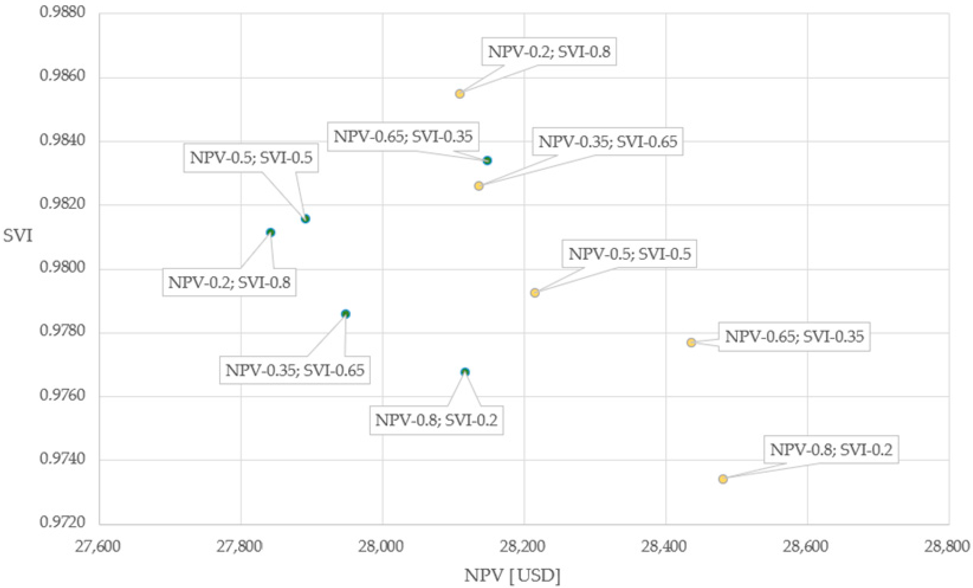
As shown in Figure 11, the results obtained after using artificial neural networks (AMTANN) showed less variation and generally had better performance (greater average distance from the center of the coordinate system). It is worth noting that the AMTANN procedure preserves the original results for later comparison with the final results. As a result, the solution with the highest NPV value (obtained for NPV-0.65; SVI-0.35 weights—green in Figure 11) was not lost. The results obtained after applying the ANN form a Pareto front, and the location of individual solutions on the graph (Figure 12) corresponds to the values of weights assumed in the objective function (the same cannot be said about the original solutions). This is typical for common trade-off problems [18].
3.1.6. Project Selection
In the last step of the procedure, the primary and ANN-modified results were selected in order to form a Pareto front (Figure 13). These results represent a range of possible versions of the project. The decision maker must choose one of these options or decide to abandon the project altogether.
As previously mentioned, a multi-criteria decision-making method can be used to make the final selection. In this case, the authors chose the most sustainable variant with the highest SVI (accepting the associated NPV value). The schedule for the selected variant is shown in Figure 14, and the selected variants of works are listed in Table 11.
3.2. Additional Tests
The effectiveness of the AMTANN procedure has been confirmed many times [16,28]. Nevertheless, for the example examined in this article, authors decided to perform additional tests. The averaged results are shown in Figure 15. On average, the results obtained after using artificial neural networks (ANNs) have higher values for NPV (Net Present Value) and SVI (Sustainability Value Index). In addition, they are more systematic, creating a Pareto front consistent with the assigned weights.
4. Discussion
The case study presented in the article shows how metaheuristic algorithms can be combined with ANNs in order to effectively optimize a construction schedule. What is more, the schedule adheres to the sustainable requirements thanks to the inclusion of the Sustainability Value Index (SVI). According to the summary of results in Table 12, the initial solution (not feasible) was improved twice. First, by the use of metaheuristic algorithm, and then further (by almost 11%) thanks to the AMTANN procedure.
Importantly, the presented methodology gives decision makers the ability to choose from among the multiple solutions that make up the Pareto front (Figure 13).
The initial solution was not feasible ( According to equations (5) and (8), the initial CF value (179,177 USD) led to the activation of penalty and a negative OF value.
Not only was there a significant improvement in the objective function and SVI parameter (dominant in the analyzed case), the NPV indicator (crucial from the client’s economical point of view) was also improved. This fact shows that environmental and economic aspects can be successfully combined. Furthermore, meeting the conditions for sustainable development does not always have to involve a compromise, sometimes it can also be economically viable.
The presented method is flexible and allows for changes in the list of criteria. Additionally, it can be applied to projects of various sizes. A slight disadvantage may be the fact that the method requires the careful construction of a model. As a result, an experienced consultant/manager must be involved in its use. However, such practices should be common for major projects.
5. Conclusions
The sustainable ecological indicator proposed in the article (SVI) allowed for the selection of a schedule that best meets the requirements of decision makers/clients. At the same time, the economic requirements were met. It is crucial as they have a great influence on decisions made by large construction companies. This was possible thanks to the use of a mix of metaheuristic algorithms and artificial intelligence.
The tests carried out previously, and for the purposes of this article, using the AMTANN procedure, showed its effectiveness. The key to the success of the method is the fact that the algorithm does not cross out the initial solutions but uses them to compare and improve the following solutions. According to the authors, the proposed model reflects the level of complexity of construction processes to a good extent. At the same time, it allows users to be flexible and adapt the model to their own needs.
Based on the research and analyses conducted by the authors, the following conclusions were drawn:
- It is possible to improve the sustainable parameters of a construction object by using appropriate methods and algorithms.
- It is possible to model the construction schedule and to select the mode of the project most adequate to the formulated expectations of decision makers.
- It is possible to reconcile the ecological and economical aspects of construction project optimization with the use of artificial intelligence tools.
- Artificial neural networks can be effectively utilized to enhance the performance of metaheuristic algorithms and improve the outcomes of construction projects.
It is important that the flexibility of the solution proposed by the authors allows the use of various algorithms and calculation tools.
There are several limitations to the work presented in the article. One limitation is that the proposed model relies on the availability of accurate data and estimates for various parameters, such as durations, resource requirements, and technological constraints. Inaccurate or incomplete data can lead to less reliable results.
There are also limitations to the use of artificial intelligence tools, such as the possibility of bias in the data used to train the models and the need for significant computational resources.
Despite these limitations, the proposed model and its use of artificial intelligence tools offer a promising approach to optimizing construction schedules while considering both sustainable and economic parameters. There is potential for further development and refinement of the model, including the incorporation of additional factors that may impact the success of a construction project. The authors also suggest testing and comparing the performance of different optimization algorithms and AI tools in future work.
Author Contributions
Conceptualization, J.K. and J.R.; methodology, J.K. and J.R.; software, J.K. and J.R.; validation, J.K. and J.R.; formal analysis, J.K. and J.R.; investigation, J.K. and J.R.; resources, J.K. and J.R.; data curation, J.K. and J.R.; writing—original draft preparation, J.R.; writing—review and editing, J.K. and J.R.; visualization, J.R.; supervision, J.K. All authors have read and agreed to the published version of the manuscript.
Funding
This research received no external funding.
Institutional Review Board Statement
Not applicable.
Informed Consent Statement
Not applicable.
Data Availability Statement
The example presented in the article is based on the model object 1110-103 (1155) (including variants) published in the Bulletins of Building Prices (BCO) in Poland. Sekocenbud. Biuletyn cen obiektów budowlanych BCO, część I—obiekty kubaturowe, II kwartał 2018 r; Ośrodek Wdrożeń Ekonomiczno-Organizacyjnych Budownictwa „PROMOCJA” Sp. z o.o.: Otwock, Poland, 2018.
Conflicts of Interest
The author declares no conflict of interest.
Abbreviations
| List of abbreviations used in the article (in alphabetical order). | |
| AMTANN | Approach for MRCPSP Transformation with the use of Artificial Neural Networks |
| ANN | Artificial Neural Networks |
| CIB | Conseil International du Bâtiment, ang. International Council for Building |
| CIOB | Chartered Institute of Building |
| ICC | International Code Council |
| ISO | International Organization for Standardization |
| LCC | Life Cycle Cost |
| MRCPSP/MMRCPSP | Multi-Mode Resource-Constrained Project Scheduling Problem |
| MRCPSPDCF | MRCPSP with Discounted Cash Flows |
| MRC-TCT/RC-TCT/TCT | Multi-Mode Resource-Constrained Time—Cost Trade-off |
| NPV | Net Present Value |
| RCPS | Resource-Constrained Project Scheduling |
| RCPSP | Resource-Constrained Project Scheduling Problem |
| SVI | Sustainable Value Index |
| TCT | Time—Cost Trade-off |
| TS | Tabu Search |
| UPS | Unconstrained Project Scheduling |
| UPSP | Unconstrained Project Scheduling Problem |
| VE | Value Engineering |
| VM | Value Management |
References
- Böde, K.; Różycka, A.; Nowak, P. Development of a Pragmatic IT Concept for a Construction Company. Sustainability 2020, 12, 7142. [Google Scholar] [CrossRef]
- Hostetler, M. Beyond design: The importance of construction and post-construction phases in green developments. Sustainability 2010, 2, 1128–1137. [Google Scholar] [CrossRef] [Green Version]
- Ibadov, N.; Kulejewski, J.; Krzemiński, M. Fuzzy ordering of the factors affecting the implementation of construction projects in Poland. In AIP Conference Proceedings; American Institute of Physics: College Park, MD, USA, 2013; Volume 1558, pp. 1298–1301. [Google Scholar]
- Rosłon, J.; Książek-Nowak, M.; Nowak, P.; Zawistowski, J. Cash-flow schedules optimization within life cycle costing (LCC). Sustainability 2020, 12, 8201. [Google Scholar] [CrossRef]
- Sobieraj, J.; Metelski, D.; Nowak, P. PMBoK vs. PRINCE2 in the context of Polish construction projects: Structural Equation Modelling approach. Arch. Civ. Eng. 2021, 67, 551–579. [Google Scholar]
- Sobieraj, J.; Metelski, D. Project Risk in the Context of Construction Schedules—Combined Monte Carlo Simulation and Time at Risk (TaR) Approach: Insights from the Fort Bema Housing Estate Complex. Appl. Sci. 2022, 12, 1044. [Google Scholar] [CrossRef]
- Yepes, V.; García-Segura, T. (Eds.) Sustainable Construction; MDPI: Basel, Switzerland, 2021; ISBN 978-3-0365-0483-4. [Google Scholar]
- Kim, J.; Koo, C.; Kim, C.J.; Hong, T.; Park, H.S. Integrated CO2, cost, and schedule management system for building construction projects using the earned value management theory. J. Clean. Prod. 2015, 103, 275–285. [Google Scholar] [CrossRef]
- Leśniak, A.; Zima, K. Cost calculation of construction projects including sustainability factors using the Case Based Reasoning (CBR) method. Sustainability 2018, 10, 1608. [Google Scholar] [CrossRef] [Green Version]
- Nicał, A.; Anysz, H. The quality management in precast concrete production and delivery processes supported by association analysis. Int. J. Environ. Sci. Technol. 2020, 17, 577–590. [Google Scholar] [CrossRef]
- Sobieraj, J. Impact of spatial planning on the pre-investment phase of the development process in the residential construction field. Arch. Civ. Eng. 2017, 63, 113–130. [Google Scholar] [CrossRef] [Green Version]
- Kulejewski, J. Construction project scheduling with imprecisely defined constraints. In Proceedings of the Management and Innovation for a Sustainable Built Environment MISBE 2011, Amsterdam, The Netherlands, 20–23 June 2011; CIB, Working Commissions W55, W65, W89, W112; ENHR and AESP. CIB: Amsterdam, Netherlands, 2011. [Google Scholar]
- Meredith, J.R.; Shafer, S.M.; Mantel, S.J., Jr. Project Management: A Strategic Managerial Approach; John Wiley & Sons: Hoboken, NJ, USA, 2017. [Google Scholar]
- Rosłon, J.; Zawistowski, J. Construction projects’ indicators improvement using selected metaheuristic algorithms. Procedia Eng. 2016, 153, 595–598. [Google Scholar] [CrossRef] [Green Version]
- Rosłon, J.; Książek-Nowak, M.; Nowak, P. Schedules Optimization with the Use of Value Engineering and NPV Maximization. Sustainability 2020, 12, 7454. [Google Scholar] [CrossRef]
- Rosłon, J.H.; Kulejewski, J.E. A hybrid approach for solving multi-mode resource-constrained project scheduling problem in construction. Open Eng. 2019, 9, 7–13. [Google Scholar] [CrossRef]
- Krzemiński, M. Conctruction scheduling and stability of the resulting schedules. Arch. Civ. Eng. 2016, 62, 89–100. [Google Scholar] [CrossRef] [Green Version]
- Podolski, M.; Rosłon, J.; Sroka, B. The Impact of the Learning and Forgetting Effect on the Cost of a Multi-Unit Construction Project with the Use of the Simulated Annealing Algorithm. Appl. Sci. 2022, 12, 12667. [Google Scholar] [CrossRef]
- Sroka, B.; Rosłon, J.; Podolski, M.; Bożejko, W.; Burduk, A.; Wodecki, M. Profit optimization for multi-mode repetitive construction project with cash flows using metaheuristics. Arch. Civ. Mech. Eng. 2021, 21, 1–17. [Google Scholar] [CrossRef]
- Habibi, F.; Barzinpour, F.; Sadjadi, S. Resource-constrained project scheduling problem: Review of past and recent developments. J. Proj. Manag. 2018, 3, 55–88. [Google Scholar] [CrossRef]
- Kolisch, R.; Sprecher, A. PSPLIB-a project scheduling problem library: OR software-ORSEP operations research software exchange program. Eur. J. Oper. Res. 1997, 96, 205–216. [Google Scholar] [CrossRef] [Green Version]
- Van Peteghem, V.; Vanhoucke, M. An experimental investigation of metaheuristics for the multi-mode resource-constrained project scheduling problem on new dataset instances. Eur. J. Oper. Res. 2014, 235, 62–72. [Google Scholar] [CrossRef]
- Giunta, M. Assessment of the Impact of CO, NOx and PM10 on Air Quality during Road Construction and Operation Phases. Sustainability 2020, 12, 10549. [Google Scholar] [CrossRef]
- Giunta, M.; Lo Bosco, D.; Leonardi, G.; Scopelliti, F. Estimation of Gas and Dust Emissions in Construction Sites of a Motorway Project. Sustainability 2019, 11, 7218. [Google Scholar] [CrossRef] [Green Version]
- Hime, N.J.; Marks, G.B.; Cowie, C.T. A Comparison of the Health Effects of Ambient Particulate Matter Air Pollution from Five Emission Sources. Int. J. Environ. Res. Public Health 2018, 15, 1206. [Google Scholar] [CrossRef] [PubMed]
- Böhringer, C.; Jochem, P.E. Measuring the immeasurable—A survey of sustainability indices. Ecol. Econ. 2007, 63, 1–8. [Google Scholar] [CrossRef] [Green Version]
- Batista, A.A.D.S.; Francisco, A.C.D. Organizational sustainability practices: A study of the firms listed by the corporate sustainability index. Sustainability 2018, 10, 226. [Google Scholar] [CrossRef] [Green Version]
- Rosłon, J. Materials and Technology Selection for Construction Projects Supported with the Use of Artificial Intelligence. Materials 2022, 15, 1282. [Google Scholar] [CrossRef]
- Lin, G.; Shen, Q. Measuring the performance of value management studies in construction: Critical review. J. Manag. Eng. 2007, 23, 2–9. [Google Scholar] [CrossRef]
- Pritsker, A.A.B.; Waiters, L.J.; Wolfe, P.M. Multiproject scheduling with limited resources: A zero-one programming approach. Manag. Sci. 1969, 16, 93–108. [Google Scholar] [CrossRef] [Green Version]
- Ratajczak-Ropel, E. Multi-mode Resource-Constrained Project Scheduling. In Population-Based Approaches to the Resource-Constrained and Discrete-Continuous Scheduling; Springer: Cham, Switzerland, 2018; pp. 69–97. [Google Scholar]
- Talbot, F.B. Resource-constrained project scheduling with time-resource tradeoffs: The nonpreemptive case. Manag. Sci. 1982, 28, 1197–1210. [Google Scholar] [CrossRef]
- Książek, M.V.; Nowak, P.O.; Kivrak, S.; Rosłon, J.H.; Ustinovichius, L. Computer-aided decision-making in construction project development. J. Civ. Eng. Manag. 2015, 21, 248–259. [Google Scholar] [CrossRef]
- Sekocenbud. Biuletyn cen obiektów budowlanych BCO, część I—obiekty kubaturowe, II kwartał 2018 r; Ośrodek Wdrożeń Ekonomiczno-Organizacyjnych Budownictwa „PROMOCJA” Sp. z o.o.: Otwock, Poland, 2018. [Google Scholar]
Figure 1.
Approximate frequency of schedule optimization according to criteria—RCPSP—modified on a base of [20].
Figure 1.
Approximate frequency of schedule optimization according to criteria—RCPSP—modified on a base of [20].
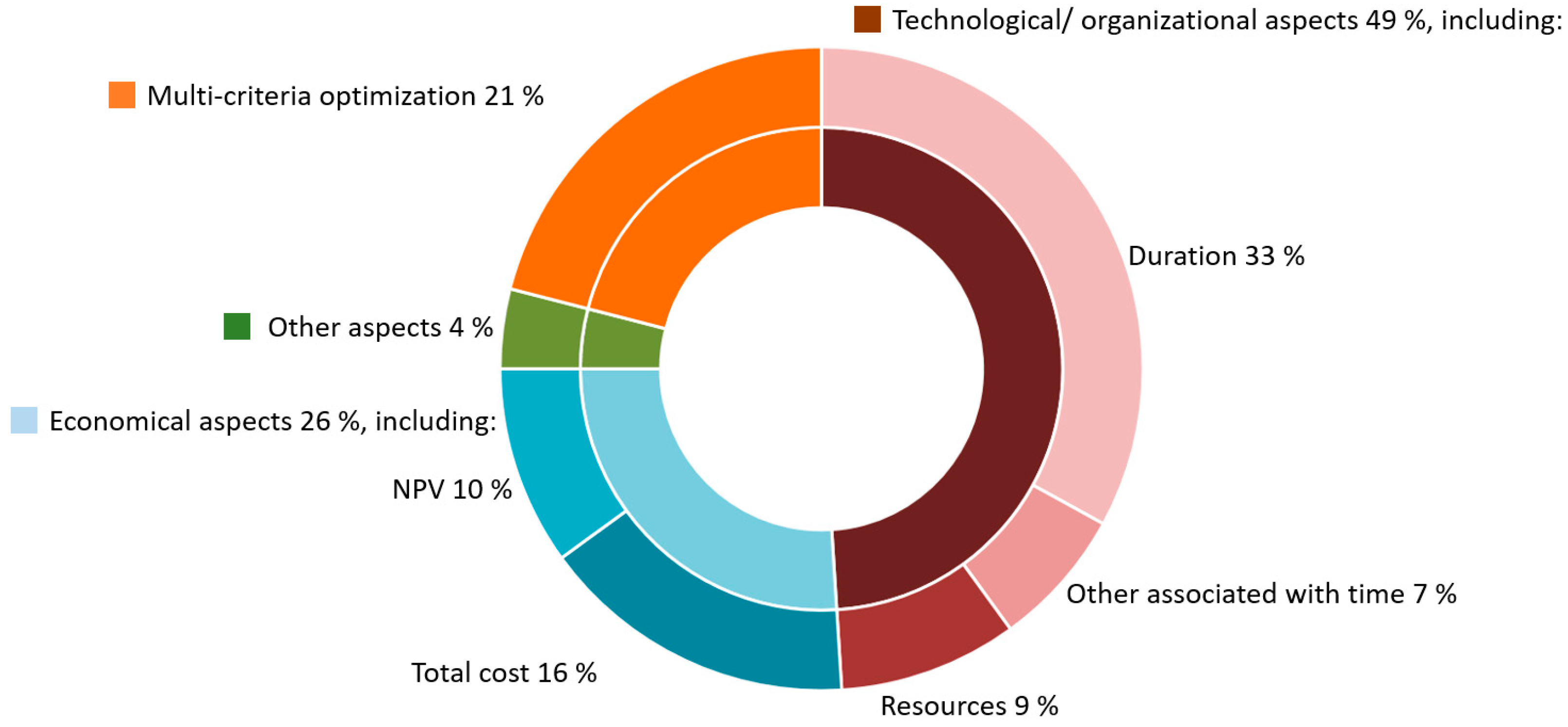
Figure 2.
Approximate frequency of schedule optimization according to criteria—MRCPSP.

Figure 3.
A diagram illustrating the steps involved in the optimization procedure.

Figure 4.
Construction project—initial schedule (presented in MS Project).
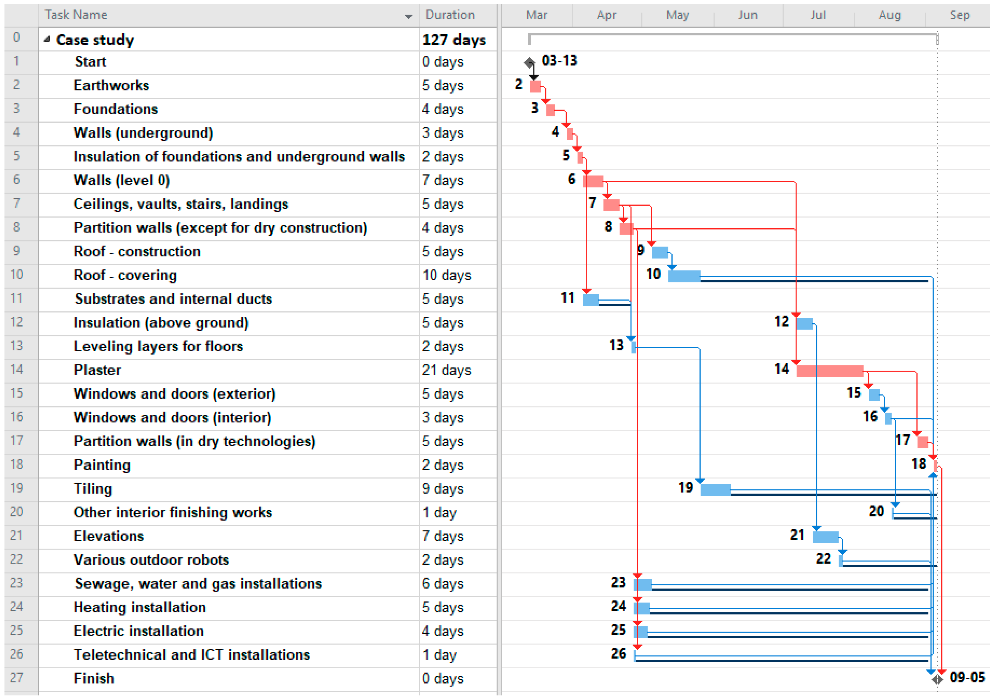
Figure 5.
The expected value of the objective function (OF) plotted as a function of the value of the decision variable being analyzed (activity 25), with the maximum values of the other variables held constant.
Figure 5.
The expected value of the objective function (OF) plotted as a function of the value of the decision variable being analyzed (activity 25), with the maximum values of the other variables held constant.
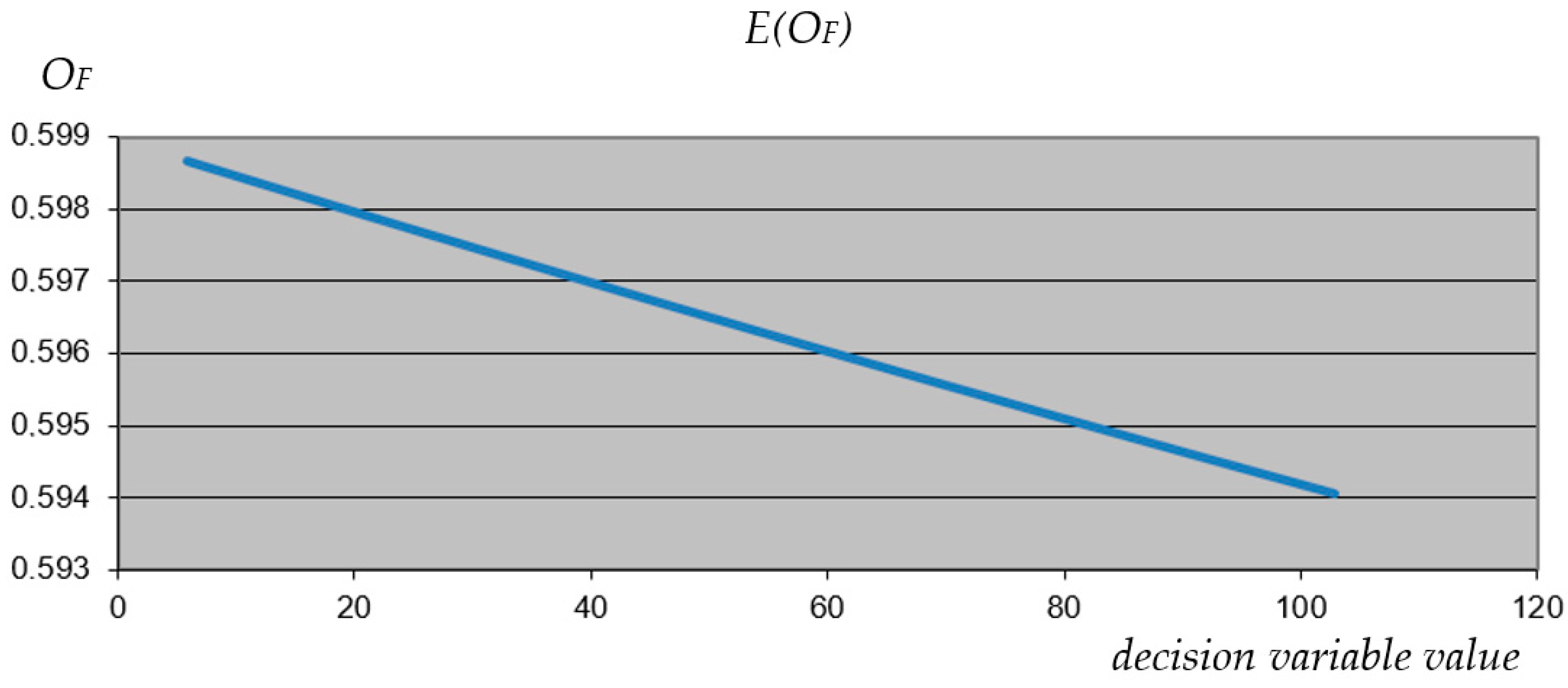
Figure 6.
The expected value of the objective function (OF) plotted as a function of the value of the decision variable being analyzed (activity 25), with the minimum values of the other variables held constant.
Figure 6.
The expected value of the objective function (OF) plotted as a function of the value of the decision variable being analyzed (activity 25), with the minimum values of the other variables held constant.
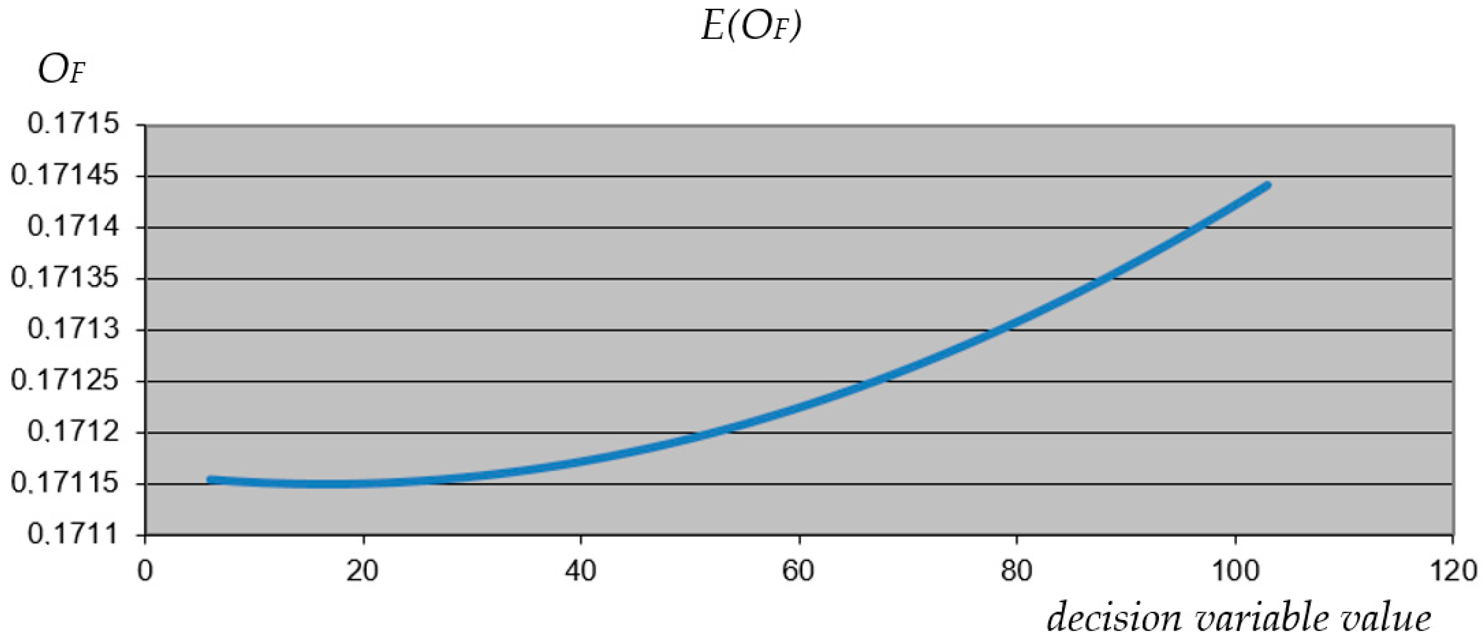
Figure 7.
The expected value of the objective function (OF) plotted as a function of the value of the decision variable being analyzed (activity 25), with the intermediate values of the other variables held constant.
Figure 7.
The expected value of the objective function (OF) plotted as a function of the value of the decision variable being analyzed (activity 25), with the intermediate values of the other variables held constant.

Figure 8.
The expected value of the objective function (OF) plotted as a function of the value of the decision variable being analyzed (activity 26), with the maximum values of the other variables held constant.
Figure 8.
The expected value of the objective function (OF) plotted as a function of the value of the decision variable being analyzed (activity 26), with the maximum values of the other variables held constant.

Figure 9.
The expected value of the objective function (OF) plotted as a function of the value of the decision variable being analyzed (activity 26), with the minimum values of the other variables held constant.
Figure 9.
The expected value of the objective function (OF) plotted as a function of the value of the decision variable being analyzed (activity 26), with the minimum values of the other variables held constant.
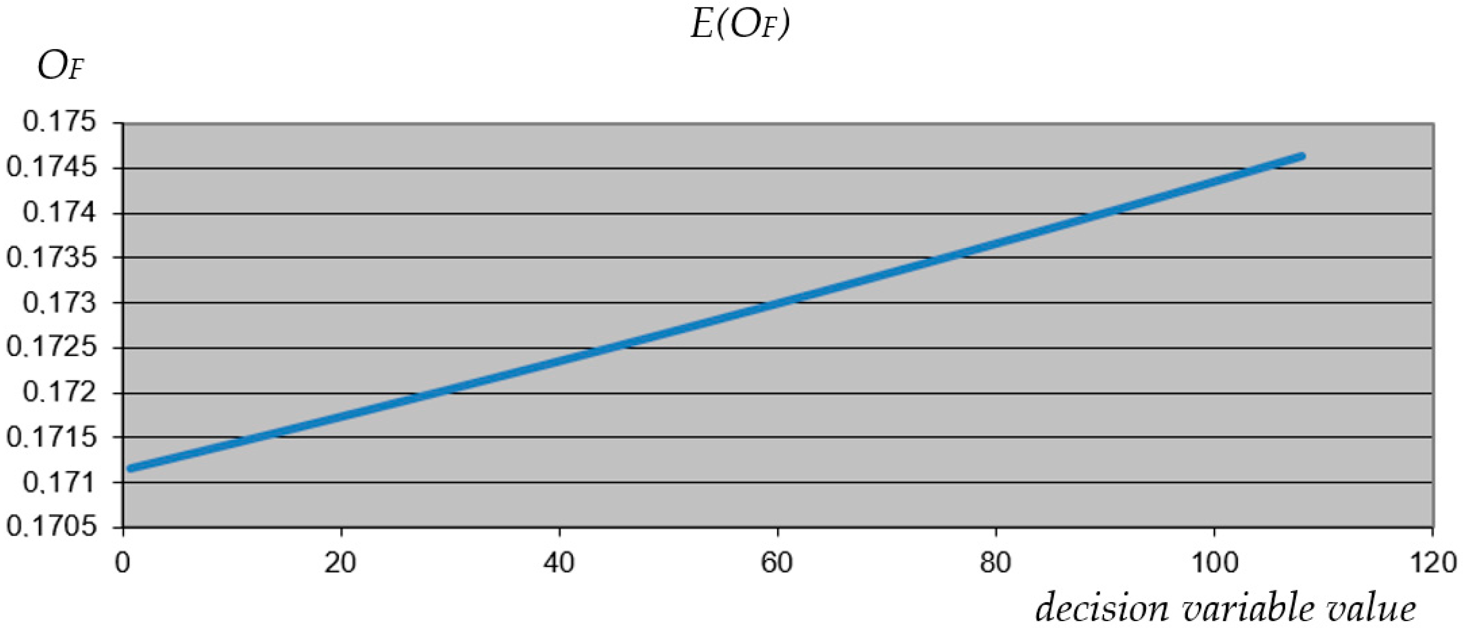
Figure 10.
The expected value of the objective function (OF) plotted as a function of the value of the decision variable being analyzed (activity 26), with the intermediate values of the other variables held constant.
Figure 10.
The expected value of the objective function (OF) plotted as a function of the value of the decision variable being analyzed (activity 26), with the intermediate values of the other variables held constant.
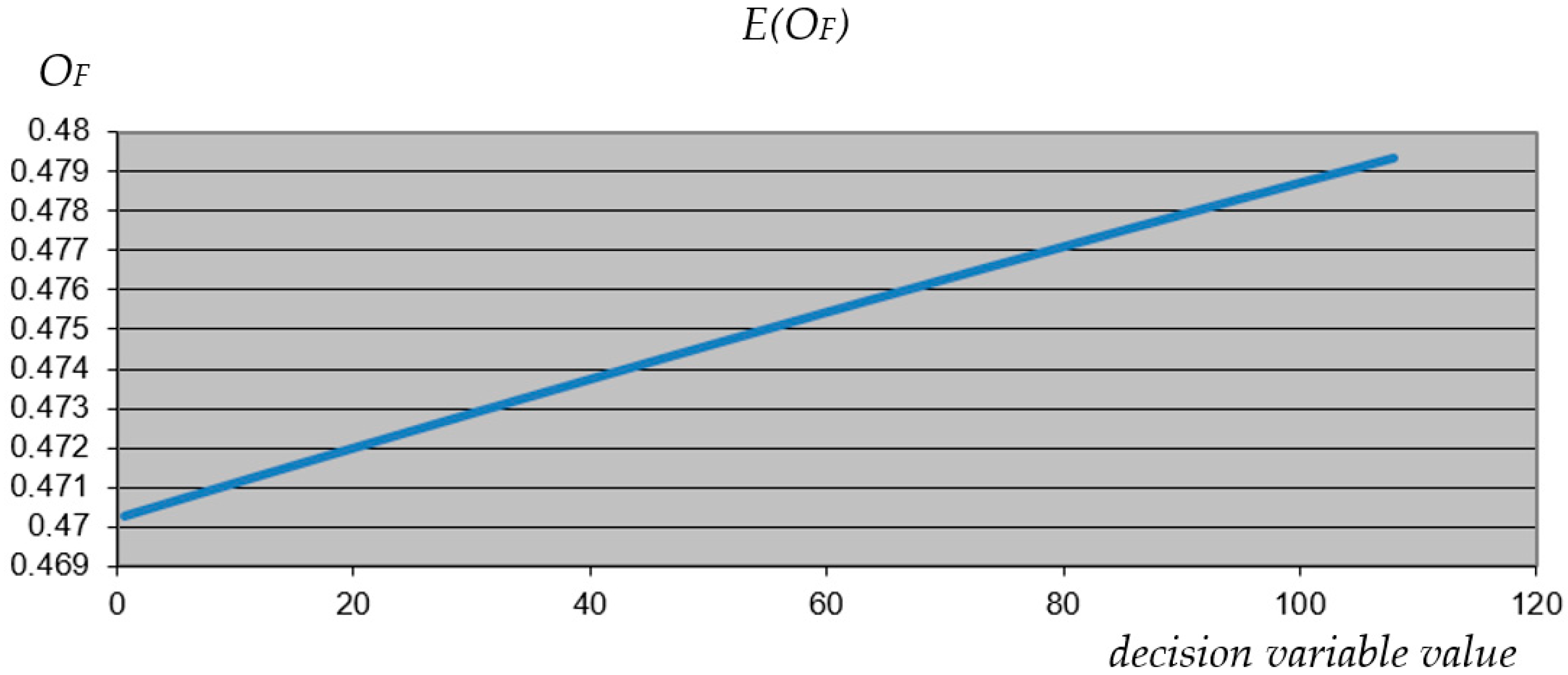
Figure 11.
Results before (green) and after (yellow) application of the AMTANN for various configurations of weights of the objective function (NPV and SVI).
Figure 11.
Results before (green) and after (yellow) application of the AMTANN for various configurations of weights of the objective function (NPV and SVI).
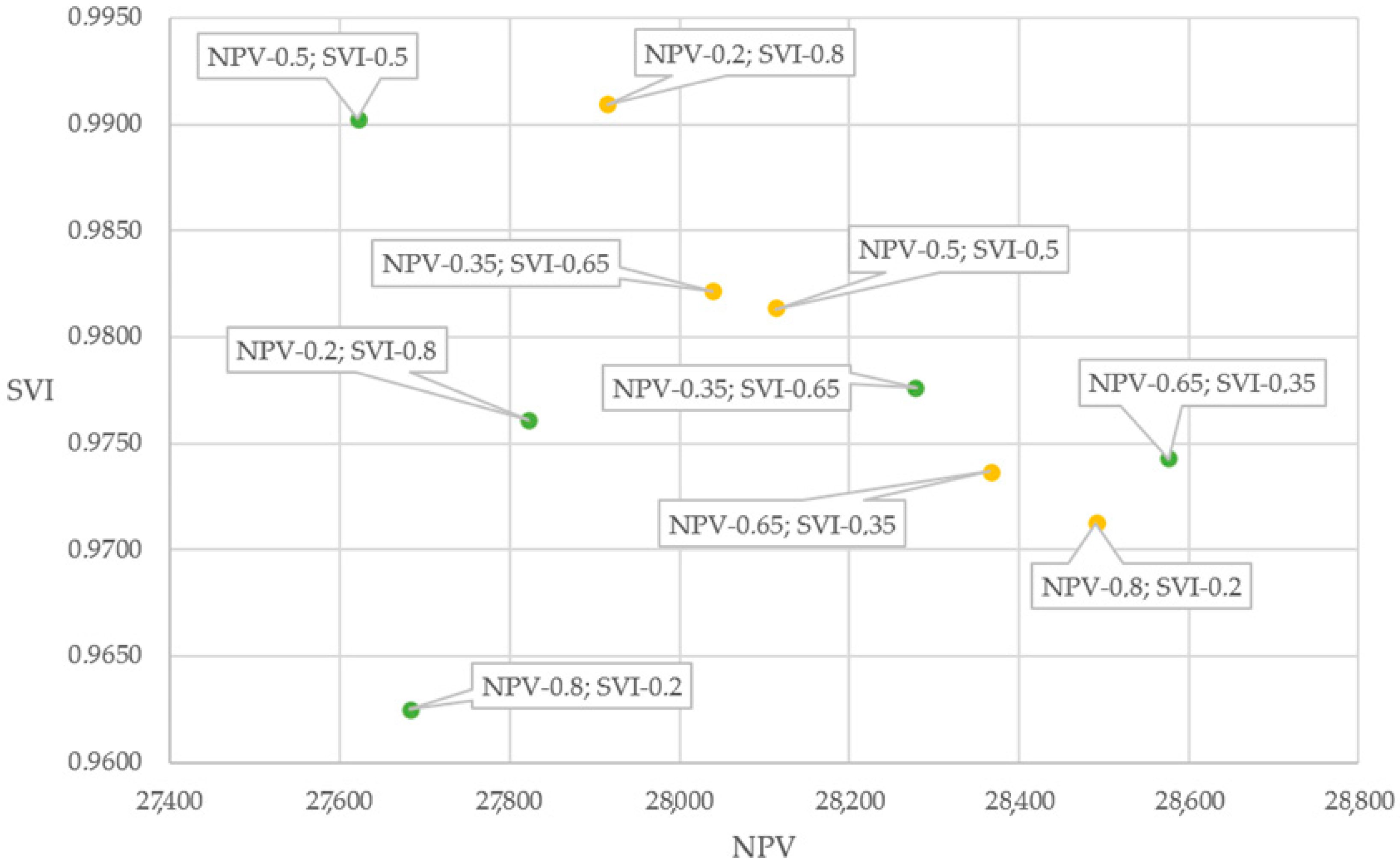
Figure 12.
The dominance area of solutions for different configurations of the weights in the objective function (NPV and SVI)—after the use of AMTANN procedure.
Figure 12.
The dominance area of solutions for different configurations of the weights in the objective function (NPV and SVI)—after the use of AMTANN procedure.

Figure 13.
The dominance area of solutions, the Pareto front—results before and after the use of AMTANN.
Figure 13.
The dominance area of solutions, the Pareto front—results before and after the use of AMTANN.
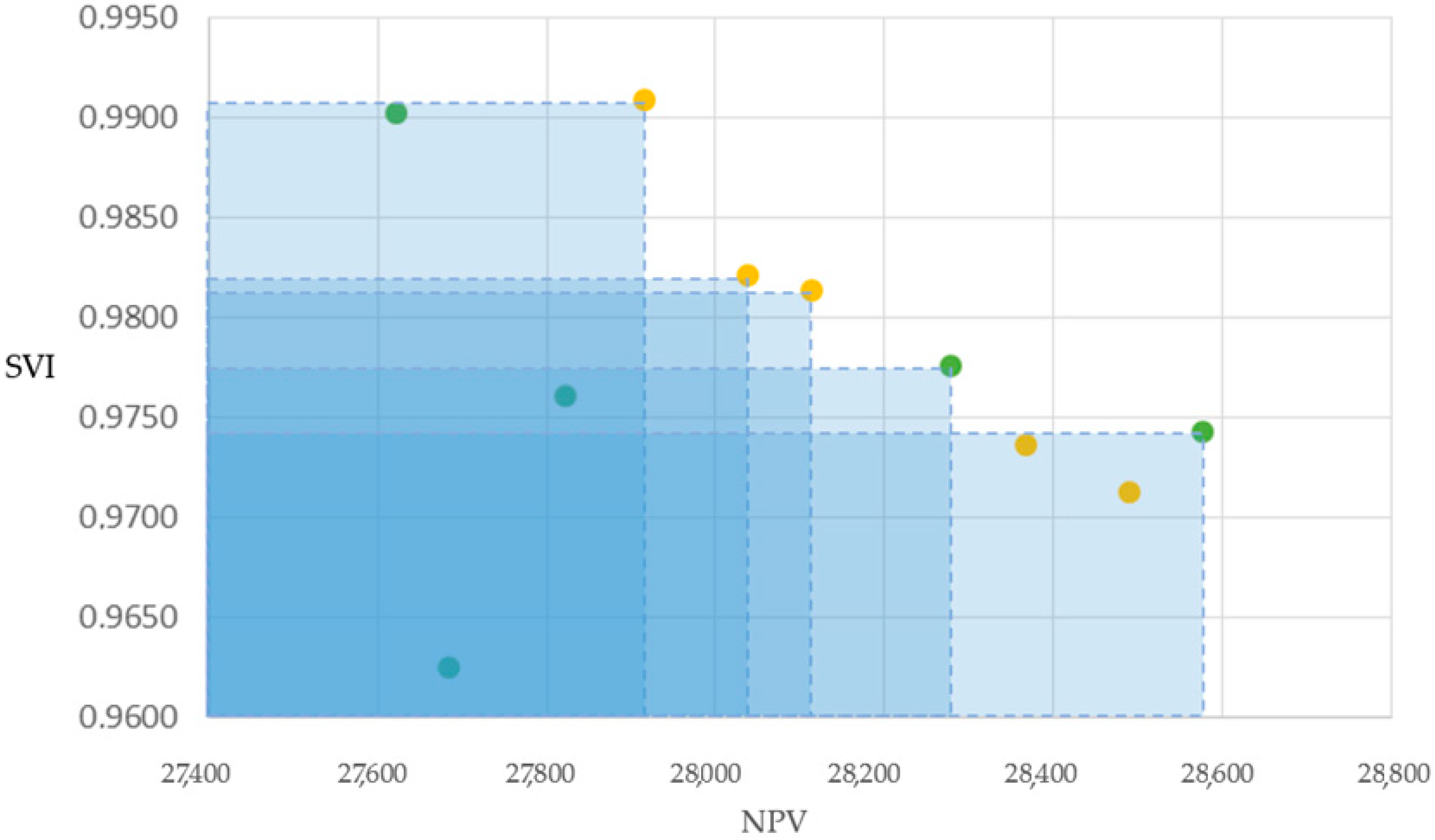
Figure 14.
Construction project—the final schedule (presented in MS Project).
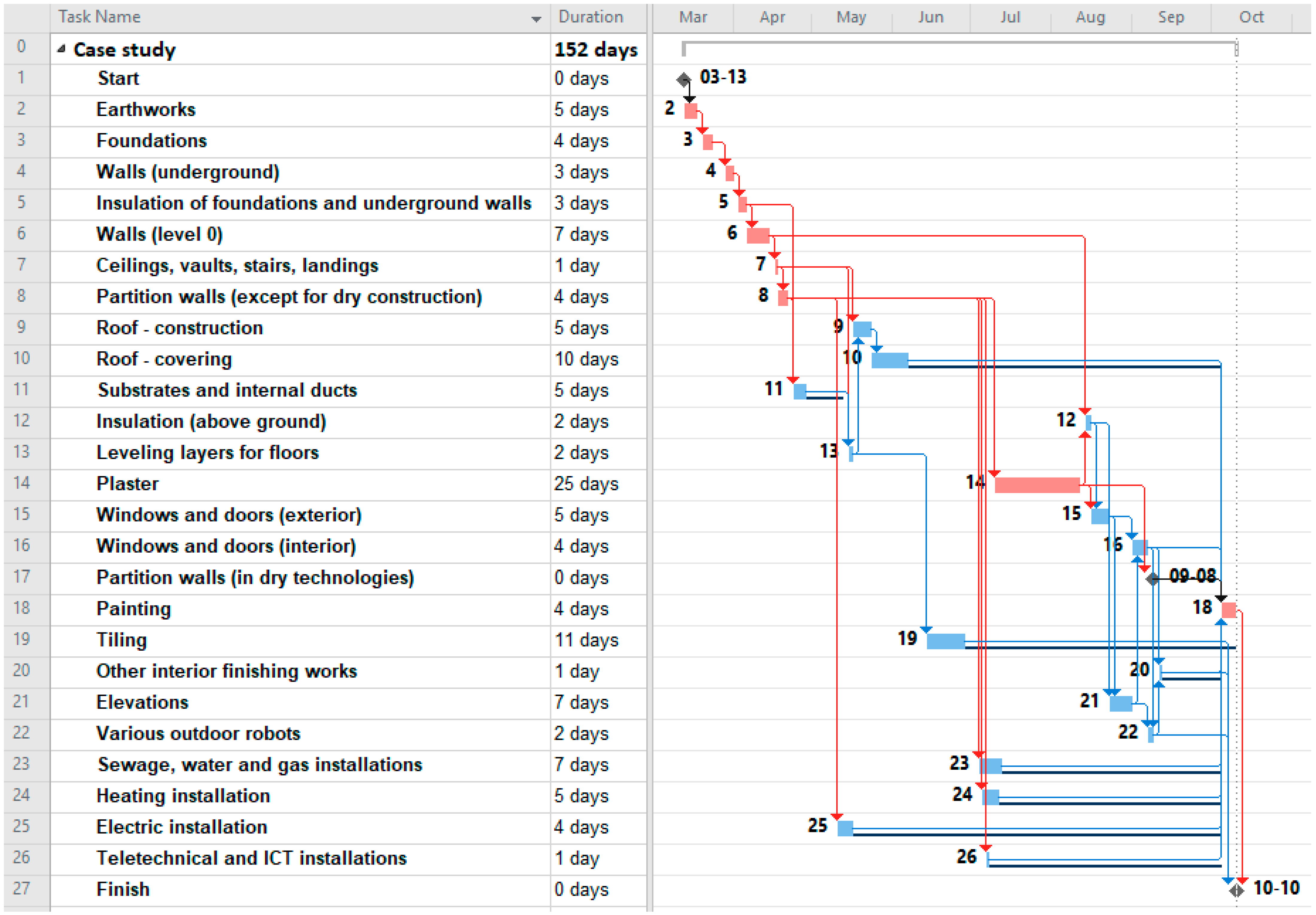
Figure 15.
Average results before (green) and after (yellow) application of AMTANN for different configurations of objective function weights (NPV and SVI).
Figure 15.
Average results before (green) and after (yellow) application of AMTANN for different configurations of objective function weights (NPV and SVI).

Table 1.
Sustainability value index—factors and sub-factors.
| 1. Sustainability | 1.1. Recycling and utilization |
| 1.2. Greenhouse gas emissions | |
| 1.3. Economics (operational costs) | |
| 1.4. Energy saving | |
| 1.5. Durability | |
| 2. User health and safety | 2.1. Air quality |
| 2.2. Water supply and other utilities | |
| 2.3. Waste disposal | |
| 3. User comfort | 3.1. Acoustic comfort |
| 3.2. Lighting (visual comfort) | |
| 3.3. Hygrothermal comfort | |
| 3.4. Serviceability |
Table 2.
A summary of the characteristics of the different variants being evaluated.
| Task | Variant 1 | Variant 2 | Variant 3 | Variant 4 | Variant 5 | |
|---|---|---|---|---|---|---|
| ID | Name | Description | Description | Description | Description | Description |
| 1 | Start | - | - | - | - | - |
| 2 | Earthworks | excavation (soil category III, groundwater level below the foundation level) | - | - | - | - |
| 3 | Foundations | monolithic, reinforced concrete | concrete blocks | brick | - | - |
| 4 | Walls (underground) | concrete blocks panels in layers and solid bricks with polystyrene thermal insulation | concrete blocks panels in layers and solid bricks with polystyrene thermal insulation; from the ground level, a pressure layer made of full clinker brick * | lime-sand blocks with thermal insulation made of mineral wool | - | - |
| 5 | Insulation of foundations and underground walls | anti-moisture (bitumen) | foil | - | - | - |
| 6 | Walls (level 0) | external: layered with checkered and cellular concrete and polystyrene tiles, internal structural: solid brick; binders and columns: monolithic—reinforced concrete | external: layered with checkerboard and polystyrene, with saturated wood filled with full construction brick (“timber framing”); internal structural: full brick; binders and columns: monolithic—reinforced concrete ** | external: layered with concrete blocks and polystyrene, with saturated wood filled with full construction brick, (“timber framing”); internal structural: full brick; binders and columns: monolithic—reinforced concrete * | external: SILKA and Styrofoam internal structural: SILKA; binders and columns: monolithic—reinforced concrete | external: Porotherm I Styrofoam internal structural: Porotherm; binders and columns: monolithic—reinforced concrete |
| 7 | Ceilings, vaults, stairs, landings | Teriva ceilings; monolithic reinforced concrete stairs | Smart ceilings; monolithic reinforced concrete stairs | ACKERMAN ceilings; monolithic reinforced concrete stairs | YTONG ceilings; monolithic reinforced concrete stairs | Filigran ceilings; monolithic reinforced concrete stairs |
| 8 | Partition walls (except for dry construction) | perforated brick *** | Silka *** | Porotherm *** | solbet (all) **** | ytong (all) **** |
| 9 | Roof—construction | wooden truss | - | - | - | - |
| 10 | Roof—covering | galvanized trapezoidal sheet; insulation: mineral wool | ceramic tile; insulation: mineral wool | bitumen tile; insulation: mineral wool; sheet metal finishes | - | - |
| 11 | Substrates and internal ducts | standard technology | - | - | - | - |
| 12 | Insulation (above ground) | Styrofoam | mineral wool | plate polyurethane | - | - |
| 13 | Leveling layers for floors | lean concrete | - | - | - | - |
| 14 | Plaster | plasters: cat. II (30%) and III (70%); glazed tiles | as in variant 1, but higher standard of materials | - | - | - |
| 15 | Windows and doors (exterior) | double-glazed PVC windows, type VEKA (71%); solid board exterior doors (14%); wooden garage doors (15%) | as in variant 1, but higher standard of materials | - | - | - |
| 16 | Windows and doors (interior) | full or glazed | as in variant 1, but higher standard of materials | - | - | - |
| 17 | Partition walls (in dry technologies) | gypsum boards on a wooden grid *** | none **** | - | - | - |
| 18 | Painting | emulsion paint | as in variant 1, but higher standard of materials | as in variant 2, but higher standard of materials | - | - |
| 19 | Tiling | ground floor: on a concrete base with terracotta tiles (31%) and oak slats (18%); utility rooms: terrazzo (15%); attic: wooden, varnished (36%) | as in variant 1, but higher standard of materials | - | - | - |
| 20 | Other interior finishing works | locksmith and blacksmith elements; balustrades | as in variant 1, but higher standard of materials | - | - | - |
| 21 | Elevations | speckled stucco, plinth faced with clinker tiles | stucco, plinth faced with clinker tiles + wooden structure painted with varnish (“timber framing”) ** | wooden structure painted with varnish (“timber framing”) (here only the painting of the facade and the execution of external balustrades are included * | - | - |
| 22 | Various outdoor robots | a band around the building made of concrete paving slabs | as in variant 1, but higher standard of materials | - | - | - |
| 23 | Sewage, water and gas installations | plastic water supply and sewage system (polypropylene and PVC) with fittings, accessories and devices. Gas installation made of steel pipes with gas cooker and oven | as in variant 1, but higher standard of materials | - | - | - |
| 24 | Heating installation | central heating installation gas boiler, convector heaters | central heating installation local gas boiler, underfloor radiators | - | - | - |
| 25 | Electric installation | switchgear with accessories, incandescent luminaires, non-tensioned lightning protection system, earthing system, TN-S electric shock protection (surface-mounted) | - | - | - | - |
| 26 | Technical and ICT installations | bell, internet, and telephone installation | as in variant 1, but higher standard of materials | - | - | - |
| 27 | Finish | - | - | - | - | - |
* Marked variants are consistent (condition T)—“timber framing” with clinker brick, i.e., if a variant marked with * is selected for any of the activities, other variants with the * symbol have to be selected in every other activity (if there is such possibility). ** Marked variants are consistent (condition T)—“timber framing” with full brick. *** Marked variants are consistent (condition T)—partial implementation of the partition walls in dry technologies was assumed. **** Marked variants are consistent (condition T)—construction of partition walls without the use of dry technologies was assumed.
Table 3.
Assessment of variants.
| Variant 1 | Variant 2 | Variant 3 | Variant 4 | Variant 5 | ||||||||||||||||
|---|---|---|---|---|---|---|---|---|---|---|---|---|---|---|---|---|---|---|---|---|
| ID | Cost [1000 USD] | Duration [Days] | SVI | Resources [Working Brigades] | Cost | Dur | SVI | Res | Cost | Dur | SVI | Res | Cost | Dur | SVI | Res | Cost | Dur | SVI | Res |
| 1 | 0.0 | 0 | 1.00 | 0 | - | - | - | - | - | - | - | - | - | - | - | - | - | - | - | - |
| 2 | 13.4 | 5 | 1.00 | 1 | - | - | - | - | - | - | - | - | - | - | - | - | - | - | - | - |
| 3 | 9.4 | 4 | 1.00 | 1 | 13.0 | 3 | 0.95 | 1 | 13.7 | 3 | 0.86 | 1 | - | - | - | - | - | - | - | - |
| 4 | 25.5 | 3 | 1.00 | 1 | 37.6 | 4 | 0.95 | 1 | 23.6 | 4 | 0.95 | 1 | - | - | - | - | - | - | - | - |
| 5 | 5.2 | 2 | 0.98 | 1 | 7.9 | 3 | 1.00 | 1 | - | - | - | - | - | - | - | - | - | - | - | - |
| 6 | 58.3 | 7 | 1.00 | 1 | 75.9 | 9 | 0.72 | 1 | 117.1 | 10 | 0.70 | 1 | 39 | 5 | 1.00 | 1 | 39 | 5 | 0.89 | 1 |
| 7 | 28.2 | 5 | 0.80 | 1 | 33.0 | 1 | 0.98 | 1 | 36.9 | 8 | 0.82 | 1 | 49.3 | 1 | 1.00 | 1 | 30.9 | 2 | 0.97 | 1 |
| 8 | 10.8 | 4 | 0.55 | 1 | 11.6 | 3 | 0.60 | 1 | 9.6 | 2 | 0.62 | 1 | 11.9 | 4 | 0.89 | 1 | 14.4 | 4 | 1.00 | 1 |
| 9 | 30.7 | 5 | 1.00 | 1 | - | - | - | - | - | - | - | - | - | - | - | - | - | - | - | - |
| 10 | 42.2 | 10 | 1.00 | 1 | 31.4 | 6 | 0.86 | 1 | 22.2 | 4 | 0.58 | 1 | - | - | - | - | - | - | - | - |
| 11 | 8.1 | 5 | 1.00 | 1 | - | - | - | - | - | - | - | - | - | - | - | - | - | - | - | - |
| 12 | 28.7 | 5 | 0.74 | 1 | 31.3 | 2 | 0.98 | 1 | 28.7 | 6 | 1.00 | 1 | - | - | - | - | - | - | - | - |
| 13 | 4.6 | 2 | 1.00 | 1 | - | - | - | - | - | - | - | - | - | - | - | - | - | - | - | - |
| 14 | 26.3 | 21 | 0.87 | 1 | 38.3 | 25 | 1.00 | 1 | - | - | - | - | - | - | - | - | - | - | - | - |
| 15 | 23.6 | 5 | 0.92 | 1 | 31.6 | 5 | 1.00 | 1 | - | - | - | - | - | - | - | - | - | - | - | - |
| 16 | 5.9 | 3 | 0.86 | 1 | 8.1 | 4 | 1.00 | 1 | - | - | - | - | - | - | - | - | - | - | - | - |
| 17 | 7.7 | 5 | 1.00 * | 1 | 0.0 | 0 | 1.00 * | 0 | - | - | - | - | - | - | - | - | - | - | - | - |
| 18 | 3.4 | 2 | 0.89 | 1 | 5.3 | 3 | 0.93 | 1 | 8.5 | 4 | 1.00 | 1 | - | - | - | - | - | - | - | - |
| 19 | 31.8 | 9 | 0.84 | 1 | 46.7 | 11 | 1.00 | 1 | - | - | - | - | - | - | - | - | - | |||
| 20 | 1.5 | 1 | 0.97 | 1 | 2.3 | 1 | 1.00 | 1 | - | - | - | - | - | - | - | - | ||||
| 21 | 15.3 | 7 | 0.95 | 1 | 16.2 | 8 | 0.76 | 1 | 2.5 | 1 | 1.00 | 1 | - | - | - | - | - | - | - | - |
| 22 | 4.0 | 2 | 0.94 | 1 | 5.3 | 2 | 1.00 | 1 | - | - | - | - | - | - | - | - | - | - | - | - |
| 23 | 21.0 | 6 | 0.72 | 0 | 30.0 | 7 | 1.00 | 0 | - | - | - | - | - | - | - | - | - | - | - | - |
| 24 | 39.9 | 5 | 0.56 | 0 | 71.1 | 5 | 1.00 | 0 | - | - | - | - | - | - | - | - | - | - | - | - |
| 25 | 20.1 | 4 | 1.00 | 0 | - | - | - | - | - | - | - | - | - | - | - | - | - | - | - | - |
| 26 | 0.4 | 1 | 0.93 | 0 | 0.9 | 1 | 1.00 | 0 | - | - | - | - | - | - | - | - | - | - | - | - |
| 27 | 0.0 | 0 | 1.00 | 0 | - | - | - | - | - | - | - | - | - | - | - | - | - | - | - | - |
* The evaluation of the SVI was carried out for task 8, therefore for task 17 the value of SVI = 1 is used for both cases.
Table 4.
Assessment of criteria and variants (evaluation matrix P)—task 7-ceilings.
| Criteria Score | V1 | V2 | V3 | V4 | V5 | ||
|---|---|---|---|---|---|---|---|
| 1. Sustainability | 1.1. Recycling and utilization | 2 | 4 | 5 | 4 | 5 | 3 |
| 1.2. Greenhouse gas emissions | 5 | 4 | 5 | 4 | 5 | 5 | |
| 1.3. Economics (operational costs) | 10 | 4 | 5 | 4 | 5 | 5 | |
| 1.4. Energy saving | 8 | 3 | 3 | 3 | 5 | 3 | |
| 1.5. Durability | 10 | 4 | 5 | 4 | 5 | 5 | |
| 2. User health and safety | 2.1. Air quality | 2 | 3 | 5 | 3 | 5 | 5 |
| 2.2. Water supply and other utilities | n/a | n/a | n/a | n/a | n/a | n/a | |
| 2.3. Waste disposal | n/a | n/a | n/a | n/a | n/a | n/a | |
| 3. User comfort | 3.1. Acoustic comfort—Rw (dB) | 3 | 48 | 54 | 49 | 40 | 53 |
| 3.2. Lighting (visual comfort) | n/a | n/a | n/a | n/a | n/a | n/a | |
| 3.3. Hygrothermal comfort | 2 | 3 | 4 | 3 | 3 | 5 | |
| 3.4. Serviceability | 2 | 3 | 4 | 5 | 2 | 4 |
Table 5.
Vector of weights Q—illustrative representation.
| Criterion | Weight |
|---|---|
| 1.1 Recycling and utilization | 0.045455 |
| 1.2 Greenhouse gas emissions | 0.113636 |
| 1.3 Economics (operational costs) | 0.227273 |
| 1.4 Energy saving | 0.181818 |
| 1.5 Durability | 0.227273 |
| 2.1 Air quality | 0.045455 |
| 2.2 Water supply and other utilities | 0 |
| 2.3 Waste disposal | 0 |
| 3.1 Acoustic comfort | 0.068182 |
| 3.2 Visual comfort (lighting) | 0 |
| 3.3 Hygrothermal comfort | 0.045455 |
| 3.4 Serviceability | 0.045455 |
Table 6.
Normalized evaluation matrix —illustrative representation.
| 1.1 | 1.2 | 1.3 | 1.4 | 1.5 | 2.1 | 2.2 | 2.3 | 3.1 | 3.2 | 3.3 | 3.4 | |
|---|---|---|---|---|---|---|---|---|---|---|---|---|
| V1 | 0.419 | 0.387 | 0.387 | 0.384 | 0.387 | 0.311 | 0.447 | 0.447 | 0.431 | 0.447 | 0.364 | 0.359 |
| V2 | 0.524 | 0.483 | 0.483 | 0.384 | 0.483 | 0.518 | 0.447 | 0.447 | 0.539 | 0.447 | 0.485 | 0.478 |
| V3 | 0.419 | 0.387 | 0.387 | 0.384 | 0.387 | 0.311 | 0.447 | 0.447 | 0.431 | 0.447 | 0.364 | 0.598 |
| V4 | 0.524 | 0.483 | 0.483 | 0.64 | 0.483 | 0.518 | 0.447 | 0.447 | 0.216 | 0.447 | 0.364 | 0.239 |
| V5 | 0.314 | 0.483 | 0.483 | 0.384 | 0.483 | 0.518 | 0.447 | 0.447 | 0.539 | 0.447 | 0.606 | 0.478 |
Table 7.
Assessment matrix SVI—illustrative representation.
| 1.1 | 1.2 | 1.3 | 1.4 | 1.5 | 2.1 | 2.2 | 2.3 | 3.1 | 3.2 | 3.3 | 3.4 | |
|---|---|---|---|---|---|---|---|---|---|---|---|---|
| V1 | 0.839 | 1.933 | 3.867 | 3.073 | 3.867 | 0.622 | 0 | 0 | 1.294 | 0 | 0.728 | 0.717 |
| V2 | 1.048 | 2.417 | 4.834 | 3.073 | 4.834 | 1.037 | 0 | 0 | 1.617 | 0 | 0.97 | 0.956 |
| V3 | 0.839 | 1.933 | 3.867 | 3.073 | 3.867 | 0.622 | 0 | 0 | 1.294 | 0 | 0.728 | 1.195 |
| V4 | 1.048 | 2.417 | 4.834 | 5.121 | 4.834 | 1.037 | 0 | 0 | 0.647 | 0 | 0.728 | 0.478 |
| V5 | 0.629 | 2.417 | 4.834 | 3.073 | 4.834 | 1.037 | 0 | 0 | 1.617 | 0 | 1.213 | 0.956 |
Table 8.
SVI assessment of ceiling variants for activity 7 of the schedule.
| Variant | SVI Score |
|---|---|
| V1—Teriva | 0.801 |
| V2—Smart | 0.983 |
| V3—ACKERMAN | 0.824 |
| V4—YTONG | 1.000 |
| V5—Filigran | 0.975 |
Table 9.
UPS optimization—extreme values of NPV, and SVI.
| Indicator | Value |
|---|---|
| 32 308 USD | |
| 20 925 USD | |
| 1.000 | |
| 0.858 |
Table 10.
The results of the analysis for different configurations of weights, both before and after using the AMTANN procedure.
Table 10.
The results of the analysis for different configurations of weights, both before and after using the AMTANN procedure.
| (NPV) | 0.8 | 0.2 | 0.65 | 0.35 | 0.5 |
| (SVI) | 0.2 | 0.8 | 0.35 | 0.65 | 0.5 |
| Before use of AMTANN | |||||
| NPVr | 0.6019 | 0.6138 | 0.6788 | 0.6531 | 0.5966 |
| SVIr | 0.7353 | 0.8311 | 0.8187 | 0.8421 | 0.9313 |
| CFr | 0.0684 | 0.0652 | 0.0667 | 0.0672 | 0.0579 |
| OF | 0.6286 | 0.7877 | 0.7277 | 0.7760 | 0.7639 |
| Duration [d] | 148 | 144 | 154 | 142 | 149 |
| NPV [USD] | 27,683 | 27,822 | 28,576 | 28,278 | 27,621 |
| SVI | 0.9625 | 0.9761 | 0.9743 | 0.9776 | 0.9903 |
| CF [USD] | 99,250 | 98,344 | 98,782 | 98,917 | 96,273 |
| After use of AMTANN | |||||
| NPVr | 0.6714 | 0.6218 | 0.6608 | 0.6325 | 0.6389 |
| SVIr | 0.7971 | 0.9362 | 0.8139 | 0.8742 | 0.8684 |
| CFr | 0.0670 | 0.0704 | 0.0600 | 0.0565 | 0.0634 |
| OF | 0.6966 | 0.8733 | 0.7143 | 0.7896 | 0.7536 |
| Duration [d] | 149 | 152 | 149 | 144 | 144 |
| NPV [USD] | 28,491 | 27,915 | 28,367 | 28,038 | 28,113 |
| SVI | 0.9713 | 0.9910 | 0.9736 | 0.9822 | 0.9814 |
| CF [USD] | 98,846 | 99,821 | 96,852 | 95,864 | 97,826 |
Table 11.
Final selection of variants.
| ID | Task Name | Selected Variant (Mode) |
|---|---|---|
| 1 | Start | 1 |
| 2 | Earthworks | 1 |
| 3 | Foundations | 1 |
| 4 | Walls (underground) | 1 |
| 5 | Insulation of foundations and underground walls | 2 |
| 6 | Walls (level 0) | 1 |
| 7 | Ceilings, vaults, stairs, landings | 2 |
| 8 | Partition walls (except for dry construction) | 5 |
| 9 | Roof—construction | 1 |
| 10 | Roof—covering | 1 |
| 11 | Substrates and internal ducts | 1 |
| 12 | Insulation (above ground) | 2 |
| 13 | Leveling layers for floors | 1 |
| 14 | Plaster | 2 |
| 15 | Windows and doors (exterior) | 1 |
| 16 | Windows and doors (interior) | 2 |
| 17 | Partition walls (in dry technologies) | 2 |
| 18 | Painting | 3 |
| 19 | Tiling | 2 |
| 20 | Other interior finishing works | 2 |
| 21 | Elevations | 1 |
| 22 | Various outdoor robots | 1 |
| 23 | Sewage, water, and gas installations | 2 |
| 24 | Heating installation | 2 |
| 25 | Electric installation | 1 |
| 26 | Technical and ICT installations | 2 |
| 27 | Finish | 1 |
Table 12.
Results summary—comparison.
| Metaheuristic Optimization Results | Initial Solution | ||
|---|---|---|---|
| After AMTANN | Before AMTANN | ||
| OF | 0.8733 | 0.7877 | not feasible |
| NPV [USD] | 27,915 | 27,822 | 23,892 |
| SVI | 0.9910 | 0.9761 | 0.896 |
| CF [USD] | 99,821 | 98,344 | 179,177 |
Disclaimer/Publisher’s Note: The statements, opinions and data contained in all publications are solely those of the individual author(s) and contributor(s) and not of MDPI and/or the editor(s). MDPI and/or the editor(s) disclaim responsibility for any injury to people or property resulting from any ideas, methods, instructions or products referred to in the content. |
© 2023 by the authors. Licensee MDPI, Basel, Switzerland. This article is an open access article distributed under the terms and conditions of the Creative Commons Attribution (CC BY) license (https://creativecommons.org/licenses/by/4.0/).
Share and Cite
MDPI and ACS Style
Kulejewski, J.; Rosłon, J. Optimization of Ecological and Economic Aspects of the Construction Schedule with the Use of Metaheuristic Algorithms and Artificial Intelligence. Sustainability 2023, 15, 890. https://doi.org/10.3390/su15010890
AMA Style
Kulejewski J, Rosłon J. Optimization of Ecological and Economic Aspects of the Construction Schedule with the Use of Metaheuristic Algorithms and Artificial Intelligence. Sustainability. 2023; 15(1):890. https://doi.org/10.3390/su15010890
Chicago/Turabian StyleKulejewski, Janusz, and Jerzy Rosłon. 2023. "Optimization of Ecological and Economic Aspects of the Construction Schedule with the Use of Metaheuristic Algorithms and Artificial Intelligence" Sustainability 15, no. 1: 890. https://doi.org/10.3390/su15010890
Note that from the first issue of 2016, this journal uses article numbers instead of page numbers. See further details here.