An Integrated Location–Scheduling–Routing Framework for a Smart Municipal Solid Waste System

Abstract

In recent decades, the explosion of the waste generation rate and corresponding environmental impacts worldwide have turned waste management into one of the most vital services in urban areas to alleviate the waste-related issues. In this study, a novel integrated model is developed to improve the municipal solid waste system by considering the facility location, shift scheduling, and vehicle routing decisions. The problem is formulated as a tri-objective mixed-integer linear programming model, striving to optimize the sustainable development goals in the waste system. These objectives encompass the total profit, air pollution emissions, citizen satisfaction, and social risk factors. The findings from this study illustrate that the proposed integrated framework empowers decision makers to maintain the resilience of the municipal solid waste system by concurrently addressing three critical sustainability aspects.

1. Introduction

The rate of global trash generation has significantly increased as a result of the tremendous development in population and manufacturing industries over the past few decades. According to projections, the amount of garbage produced annually will rise from 2 billion tons in 2016 to over 3.4 billion tons in 2050 [1]. A complicated challenge, managing this enormous volume of waste calls for careful consideration of issues including transportation planning, crew scheduling, public health, and social issues [2]. Inadequate waste management can have negative effects, including risks to public health, the depletion of natural resources, and environmental deterioration [3]. Therefore, it becomes crucial to develop an effective and sustainable waste system that considers pragmatic factors like public health principles and garbage collection hurdles. This study focuses on municipal solid waste (MSW) management to reduce the consequences of solid waste generation issues.

Numerous research addressing various waste systems, including waste container collection, the distribution of sorted materials, and facility location has been undertaken and published in the literature on waste management (WM). However, the majority of these studies have dealt with facility location, shift scheduling, or vehicle routing independently rather than combining them into a single framework. To improve the route and scheduling of waste collection, for instance, Tung and Pinnoi (2000) suggested a mixed integer programming (MIP) model, focusing on the overall cost and the number of trucks [4]. Hemmelmayr et al. (2013) investigated vehicle routing problem (VRP) models for periodic multi-depot garbage collection time optimization [5]. These research studies prioritized the various elements, leaving room for an integrated approach.

Smart waste systems can now be developed by utilizing sensor-based and data transmission technologies due to the rapid expansion of information and communication technologies (ICT) and the Internet of Things (IoT) technologies [6]. As an illustration, Fan et al. (2010) suggested a routing model that incorporates intelligent sensors and a Geographic Information System (GIS) to monitor garbage containers with an emphasis on vehicle energy utilization [7]. Using a capacitated VRP model, Akhtar et al. (2017) developed the smart bins’ garbage collection path [8]. These studies highlight the crucial part that cutting-edge technologies play in trash management. However, they also stress the necessity for a more thorough strategy that incorporates several waste management system components.

Table 1. Summary of the literature on municipal solid waste.

Refs.	Problem			Modeling Approach	Objectives	IoT	Sustainability			Solution Methodology
	VRP	Shift Scheduling	Facility Location				Economic	Environmental	Social
[4]	✓	✓		MIP	O2-O5		✓			Heuristic
[5]	✓			MIP	O3		✓			Hybrid VNS and Dynamic programming
[7]	✓			MINLP	O4-O10	✓				Hybrid GA-SA
[8]	✓			MILP	O4-O8	✓	✓			Modified BSA
[9]	✓			MILP	O3-O5					Heuristic
[10]	✓			$-$	O4-O5					Simulation
[11]	✓			MILP	O4-O6-O11		✓	✓	✓	Exact
[12]	✓		✓	MILP	O1-O8		✓			Heuristic
[13]			✓	MILP	O1-O11		✓	✓	✓	Exact
[14]	✓	✓		$-$	O2		✓			Simheuristic approach
[15]	✓			MILP	O2-O4		✓			Hybrid heuristic approach
[16]	✓			MILP	O9					Exact
[17]			✓	RO	O2-O11		✓	✓		Exact
[18]	✓			NLP	O2-O7-O9		✓	✓	✓	MOSAEA algorithm
[19]	✓			$-$	O3-O4-O8-O9	✓				Heuristics
[20]	✓			MINLP	O1-O2-O4-O5-O11	✓	✓	✓	✓	Metaheuristic and hybrid algorithms
Current study	✓	✓	✓	MILP	O1-O7-O10-O11	✓	✓	✓	✓	Exact

O1: Profit or recovery value; O2: Total cost; O3: Time; O4: Route distance; O5: Number of vehicles; O6: Workload balance of vehicles or facilities; O7: Risk; O8: Quantity of collected waste; O9: Fuel or energy consumption; O10: Energy generation; O11: Emissions, pollutants, and/or potential harm.

summarizes the recent literature on the municipal solid waste. This study aims to bridge the gap in the literature by proposing an integrated location–scheduling–routing framework for a smart municipal solid waste system. The research questions that guide this study are: Can we develop an integrated model that simultaneously considers facility location, shift scheduling, and vehicle routing decisions in the municipal solid waste system? How would such an integrated model affect the total profit, air pollution emissions, social risk factors, and citizens’ satisfaction?

Our objective is to develop a multi-echelon multi-objective optimization model to optimize the total network profit, air pollution emissions, social risk factors, and the satisfaction of citizens. In other words, this research aims to provide an integrated framework that enables managers and decision makers to evaluate the impact of main decisions within different planning horizons on each other in order to administer the operations of a waste network efficiently while considering the sustainable development goals. This research contributes to the body of knowledge by providing an integrated model for waste management, thereby bringing a new perspective to tackling the challenges associated with waste management.

The rest of this study is organized as follows. Section 2 describes the problem under study and illustrates the main assumptions of the problem. The formulation of the multi-objective model and the required linearization and transformation techniques are explained in Section 3. The proposed solution approach for addressing the multi-objectiveness of the mathematical model is presented in Section 4. In Section 5, the applicability of the optimization model and validation of the solution approach are examined using real-world examples. Then, the sensitivity analysis of the influential parameters is discussed. Ultimately, the main findings of this study are summarized, and some future research avenues are provided in Section 6.

2. Problem Description and Assumptions

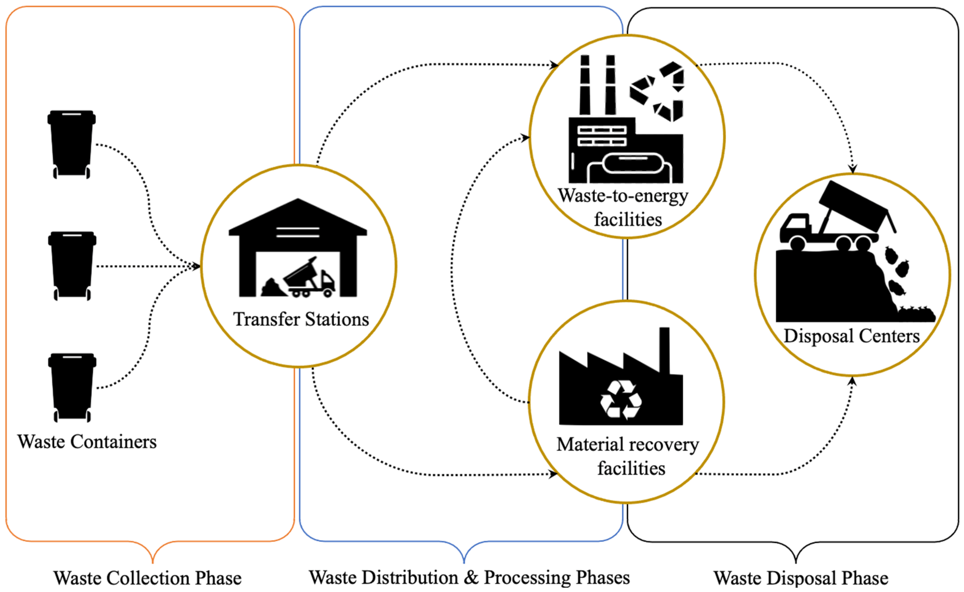
In this study, to address some of the research gaps that exist in the MSW literature, an integrated optimization model is developed that incorporates facility location, shift scheduling, and vehicle routing (LSR) problems, which aims to boost the performance of the current waste systems using IoT technologies. The elements of the proposed multi-echelon MSW network comprise waste generation points, collection centers, transfer stations, MRFs, WTEFs, and disposal centers. In some previous studies, the waste network was divided into smaller zones, and it was assumed that all waste generation points are assigned to the corresponding collection center in a specific region (e.g., [21]). This study assumes that there is no pre-assignment of waste generation nodes to a specific transfer station, which leads to a more static collection plan. This assumption makes the problem more realistic and enables decision makers (DMs) to provide more dynamic scheduling and routing plans considering the available workforce, facilities, and vehicles. The framework of the multi-echelon MSW network is shown in Figure 1.

The first two levels of the network relate to the waste collection phase, in which the collected waste materials from the generation nodes are transported and stored in a transfer station. In the waste network, transfer stations are connected with MRFs and WTEFs applied, respectively, in sorting/recovering recyclable items (e.g., paper, plastic, glass) and generating energy from waste residues. Finally, the remaining portion of non-recyclable and non-recoverable waste residues at MRFs and WTEFs are transferred to the disposal centers. In the proposed network, to find the optimal collection and allocation decisions in the municipal area, a VRP considering time window constraints and heterogeneous fleets of vehicles is formulated to determine the optimal flow of waste throughout the network. In the LSR model, the main components in the operational planning scale include the allocation, routing, and shift scheduling decisions which are made at the lower level of the decision-making hierarchy. The waste materials generated throughout the municipal area should be handled using these components to improve the economic, environmental, and social impacts within the short-term planning horizon. In addition to these decisions, the other key component of the waste system in this study is the facility location decision which determines the best possible locations of MRFs and WTEFs. Contrary to the first group of components, the facility location decision is made within the strategic planning horizon which is considered as a long-term or even one-time type of decision. Due to the high construction, establishment, and installation costs of processing facilities in practice, these strategic decisions occur at a corporate level and must be taken at the upper level of the decision-making hierarchy to ensure the sustainability of the waste system. These two groups of decisions are generally taken in different time scales and by different levels of DMs; however, they have a major impact on each other. The goal of this study is to incorporate operational and strategic decisions in an integrated model to analyze the influence of these decisions on each other and reveal how sustainability can be improved. The remaining main assumptions of the proposed LSR problem are briefly illustrated as follows:

• A certain number of potential locations for the MRFs and WTEFs are identified in the MSW network, and a limited number of them can be established at the beginning of the planning horizon.
• A waste container is collected if its fill-level exceeds a predefined TWL, which avoids the unnecessary collection of containers.
• In the collection phase, each container must be served by only one vehicle and on a single visit.
• Each vehicle completes only one trip in a working shift; however, it might be employed in multiple shifts during the planning horizon.
• A preferred time window is determined for the collection of waste containers, and any earliness or tardiness in service provision is penalized by a constant rate which shows the dissatisfaction of customers.
• All collection trucks must return to the same center that they started their trips from, when all allocated points are served, or the vehicle’s load capacity is reached.
• All the parameters of the optimization model are deterministic and assumed to be known to DMs.
• Each waste container is equipped with IoT technologies, including weight and volume sensors, automatic actuator, RFID tag, and GPRS. The provided equipment enables the waste system to monitor the weight and fill-level of waste bins and prevent the disposal of waste when a container is full.

3. Mathematical Model

The mathematical model of the LSR problem is demonstrated in this section, aiming to optimize the management of municipal solid waste and related operations in line with the assumptions stated in Section 2. The mathematical notations of the model are introduced in

Table 2. Sets and indices in the mathematical model.

Index	Definition
i	Waste generation nodes (containers); $\mathrm{i}\in \mathrm{I}$
j	Transfer stations; $\mathrm{j}\in \mathrm{J}$
$\mathrm{d}$	Disposal centers; $\mathrm{d}\in \mathrm{D}$
$\mathrm{r}$	Candidate sites for establishment of MRFs; $\mathrm{r}\in \mathrm{R}$
$\mathrm{q}$	Candidate sites for establishment of WTEFs; $\mathrm{q}\in \mathrm{Q}$
$\mathrm{u}$	Nodes in the set of processing facilities; $\mathrm{u}\in \mathrm{U}=\{\mathrm{R}\cup \mathrm{Q}\}$
n1, n2	Nodes in the set of points including transfer stations and waste containers; ${\mathrm{n}}_1,{\mathrm{n}}_2$ $\in \mathrm{N}=\{\mathrm{I}\cup \mathrm{J}\}$
$\mathrm{w}$	Recyclable waste types; 𝑤∈𝑊
$\mathrm{p}$	Products produced in the recovery processes at WTEF; $\mathrm{p}\in \mathrm{P}$
$\mathrm{v}$	Waste trucks at a transfer station; $\mathrm{v}\in {\mathrm{V}}_{\mathrm{j}}=\{1,\dots ,{\mathrm{n}\mathrm{v}}_{\mathrm{j}}\}$
$\mathrm{e}$	Types of air pollutant emission; $\mathrm{e}\in \mathrm{E}$
$\mathrm{s}$	Shift types of waste trucks; $\mathrm{s}\in \mathrm{S}$

,

Table 3. Parameters in the mathematical model.

Parameter	Definition
${\mathrm{n}\mathrm{v}}_{\mathrm{j}}$	Number of waste trucks at transfer station $\mathrm{j}$
${\mathrm{c}\mathrm{c}\mathrm{a}\mathrm{p}}_{\mathrm{i}}$	Capacity of container $\mathrm{i}$ ($\mathrm{t}\mathrm{o}\mathrm{n}$)
${\mathrm{w}\mathrm{t}\mathrm{c}\mathrm{a}\mathrm{p}}_{\mathrm{v},\mathrm{j}}$	Capacity of waste truck $\mathrm{v}$ at transfer station $\mathrm{j}$ ($\mathrm{t}\mathrm{o}\mathrm{n}$)
$\mathrm{w}\mathrm{l}\mathrm{t}$	Weight of an empty waste truck
$\mathrm{w}\mathrm{h}\mathrm{t}$	Weight of an empty high-capacity trailer
$\mathrm{t}\mathrm{r}{\mathrm{c}\mathrm{a}\mathrm{p}}_{\mathrm{j}}$	Capacity of transfer station $\mathrm{j}$ ($\mathrm{t}\mathrm{o}\mathrm{n}$)
${\mathrm{m}\mathrm{r}\mathrm{f}\mathrm{c}\mathrm{a}\mathrm{p}}_{\mathrm{r}}$	Capacity of MRF $\mathrm{r}$ to separate recyclables ($\mathrm{t}\mathrm{o}\mathrm{n}$)
$\mathrm{w}\mathrm{t}\mathrm{e}{\mathrm{c}\mathrm{a}\mathrm{p}}_{\mathrm{q}}$	Capacity of WTEF $\mathrm{q}$ in processing non-recyclable waste ($\mathrm{t}\mathrm{o}\mathrm{n}$)
${\mathrm{d}\mathrm{c}\mathrm{a}\mathrm{p}}_{\mathrm{d}}$	Capacity of disposal center $\mathrm{d}$ ($\mathrm{t}\mathrm{o}\mathrm{n}$)
${\mathrm{c}\mathrm{w}}_{\mathrm{i}}$	Weight information for container $\mathrm{i}$ reported by its weight sensor ($\mathrm{t}\mathrm{o}\mathrm{n}$)
${\mathsf{\gamma }}_{\mathrm{i}}$	TWL for waste container $\mathrm{i}$ (percent)
$[{\mathrm{l}\mathrm{t}\mathrm{w}}_{\mathrm{i}},{\mathrm{u}\mathrm{t}\mathrm{w}}_{\mathrm{i}}]$	Time window for serving container $\mathrm{i}$
${\mathrm{s}\mathrm{v}\mathrm{t}}_{\mathrm{i}}$	Service time for container $\mathrm{i}$ ($\mathrm{s}\mathrm{e}\mathrm{c}\mathrm{o}\mathrm{n}\mathrm{d}$)
${\mathrm{d}\mathrm{s}\mathrm{t}}_{{\mathrm{n}}_1,{\mathrm{n}}_2}^{\mathrm{N}}$	Distance between nodes ${\mathrm{n}}_1$ and ${\mathrm{n}}_2$ in a set including transfer stations and waste containers ($\mathrm{k}\mathrm{m}$)
${\mathrm{d}\mathrm{s}\mathrm{t}}_{{\mathrm{u}}_1,{\mathrm{u}}_2}^{\mathrm{U}}$	Distance between nodes ${\mathrm{u}}_1$ and ${\mathrm{u}}_2$ in a set including transfer stations and potential processing facilities ($\mathrm{k}\mathrm{m}$)
${\mathrm{d}\mathrm{s}\mathrm{t}}_{{\mathrm{l}}_1,{\mathrm{l}}_2}^{\mathrm{D}}$	Distance between nodes ${\mathrm{l}}_1$ and ${\mathrm{l}}_2$ in a set including potential processing facilities and disposal centers ($\mathrm{k}\mathrm{m}$)
$\mathrm{s}\mathrm{p}$	Average speed of waste trucks ($\mathrm{k}\mathrm{m}/\mathrm{h}\mathrm{o}\mathrm{u}\mathrm{r}$)
${\mathrm{t}\mathrm{n}}_{{\mathrm{n}}_1,{\mathrm{n}}_2}$	Travel time between set of points including transfer stations and waste containers $\left({\mathrm{t}\mathrm{n}}_{{\mathrm{n}}_1,{\mathrm{n}}_2}={\mathrm{d}\mathrm{s}\mathrm{t}}_{{\mathrm{n}}_1,{\mathrm{n}}_2}^{\mathrm{N}}/\mathrm{s}\mathrm{p}\right)$
${\mathrm{a}\mathrm{v}}_{\mathrm{v},\mathrm{j},\mathrm{s}}$	1: If waste truck $\mathrm{v}$ at transfer station $\mathrm{j}$ is available in shift $\mathrm{s}$; 0: Otherwise
$[{\mathrm{s}\mathrm{t}\mathrm{s}}_{\mathrm{s}},{\mathrm{e}\mathrm{n}\mathrm{s}}_{\mathrm{s}}]$	Starting and ending times in the working shift $\mathrm{s}$
$\mathrm{s}\mathrm{m}\mathrm{a}\mathrm{x}$	Maximum allowable number of shifts for waste trucks
$\mathrm{m}\mathrm{m}\mathrm{a}\mathrm{x}$	Maximum allowable number of MRFs that can be established
$\mathrm{w}\mathrm{m}\mathrm{a}\mathrm{x}$	Maximum allowable number of WTEFs that can be established
$\mathrm{f}\mathrm{c}\mathrm{w}\mathrm{t}$	Fixed cost of employing a waste truck ($\mathrm{U}\mathrm{S}\mathrm{D}$)
$\mathrm{v}\mathrm{c}\mathrm{w}\mathrm{t}$	Variable cost of employing a waste truck ($\mathrm{U}\mathrm{S}\mathrm{D}/(\mathrm{t}\mathrm{o}\mathrm{n}\times \mathrm{k}\mathrm{m})$)
$\mathrm{f}\mathrm{c}\mathrm{h}\mathrm{t}$	Fixed cost of employing a high-capacity trailer to distribute the collected waste ($\mathrm{U}\mathrm{S}\mathrm{D}$)
$\mathrm{v}\mathrm{c}\mathrm{h}\mathrm{t}$	Variable cost of employing a high-capacity trailer to distribute the collected waste ($\mathrm{U}\mathrm{S}\mathrm{D}/(\mathrm{t}\mathrm{o}\mathrm{n}\times \mathrm{k}\mathrm{m})$)
${\mathrm{e}\mathrm{s}\mathrm{c}\mathrm{m}}_{\mathrm{r}}$	Establishment cost for MRF $\mathrm{r}$ ($\mathrm{U}\mathrm{S}\mathrm{D}$)
${\mathrm{e}\mathrm{s}\mathrm{c}\mathrm{w}}_{\mathrm{q}}$	Establishment cost for WTEF $\mathrm{q}$ ($\mathrm{U}\mathrm{S}\mathrm{D}$)
${\mathrm{o}\mathrm{p}\mathrm{c}\mathrm{m}}_{\mathrm{r}}$	Operational cost in MRF $\mathrm{r}$ for separating recyclables ($\mathrm{U}\mathrm{S}\mathrm{D}/\mathrm{t}\mathrm{o}\mathrm{n}$)
${\mathrm{o}\mathrm{p}\mathrm{c}\mathrm{w}}_{\mathrm{q}}$	Operational cost in WTEF $\mathrm{q}$ for processing waste materials ($\mathrm{U}\mathrm{S}\mathrm{D}/\mathrm{t}\mathrm{o}\mathrm{n}$)
${\mathrm{d}\mathrm{c}}_{\mathrm{d}}$	Disposal cost in disposal center $\mathrm{d}$ ($\mathrm{U}\mathrm{S}\mathrm{D}/\mathrm{t}\mathrm{o}\mathrm{n}$)
$[{\mathrm{p}\mathrm{c}\mathrm{e}}_{\mathrm{i}},{\mathrm{p}\mathrm{c}\mathrm{l}}_{\mathrm{i}}]$	Penalty costs for serving container $\mathrm{i}$ earlier and later than the time window
$\mathrm{o}\mathrm{p}\mathrm{f}$	Operations fee for collection and disposal services ($\mathrm{U}\mathrm{S}\mathrm{D}$)
${\mathrm{s}\mathrm{p}\mathrm{m}}_{\mathrm{w}}$	Selling price for sorted waste type $\mathrm{w}$ at MRFs ($\mathrm{U}\mathrm{S}\mathrm{D}/\mathrm{t}\mathrm{o}\mathrm{n}$)
${\mathrm{s}\mathrm{p}\mathrm{w}}_{\mathrm{p}}$	Selling price for product type $\mathrm{p}$ at WTEFs ($\mathrm{U}\mathrm{S}\mathrm{D}/\mathrm{t}\mathrm{o}\mathrm{n}$)
$\mathrm{e}\mathrm{s}\mathrm{b}$	Total establishment budget for opening processing facilities
$\mathsf{\beta }$	Percentage of recyclables in accumulated solid waste at transfer stations (percent)
${\mathsf{\xi }}_{\mathrm{w}}$	Percentage of recyclable waste type $\mathrm{w}$ in accumulated solid waste at MRFs (percent)
${\mathsf{\omega }}_{\mathrm{p}}$	Production rate of product type $\mathrm{p}$ at WTEFs (percent)
$\mathrm{f}\mathrm{c}\mathrm{r}\mathrm{w}\mathrm{t}$	Fuel consumption rate for waste trucks (lit/km)
$\mathrm{f}\mathrm{c}\mathrm{r}\mathrm{h}\mathrm{t}$	Fuel consumption rate for high-capacity trailers (lit/km)
${\mathrm{i}\mathrm{n}\mathrm{t}\mathrm{w}}_{\mathrm{e}}$	Global warming potential intensity weight for emission type $\mathrm{e}$
${\mathrm{q}\mathrm{e}\mathrm{t}}_{\mathrm{e}}$	Quantity of emission type $\mathrm{e}$ from transportation activities (gr/(ton × lit))
${\mathrm{q}\mathrm{e}\mathrm{w}}_{\mathrm{e}}$	Quantity of emission type $\mathrm{e}$ from WTEFs’ operations (gr/ton)
${\mathrm{q}\mathrm{e}\mathrm{d}}_{\mathrm{e}}$	Quantity of emission type $\mathrm{e}$ from disposal centers (gr/ton)
${\mathrm{p}\mathrm{o}\mathrm{p}\mathrm{m}}_{\mathrm{r}}$	Population living near the potential MRF $\mathrm{r}$
${\mathrm{p}\mathrm{o}\mathrm{p}\mathrm{w}}_{\mathrm{q}}$	Population living near the potential WTEF $\mathrm{q}$
${\mathrm{o}\mathrm{d}\mathrm{m}}_{\mathrm{r}}$	Intensity of the unpleasant odor near the potential MRF $\mathrm{r}$
${\mathrm{o}\mathrm{d}\mathrm{w}}_{\mathrm{q}}$	Intensity of the unpleasant odor near the potential WTEF $\mathrm{q}$
$\mathsf{\Psi }$	A large positive number
$\mathsf{\epsilon }$	A small number
$\mathsf{\theta }$	Importance level of social risk factors

and

Table 4. Decision variables in the mathematical model.

Variable	Definition
${\mathrm{S}\mathrm{R}\mathrm{V}}_{\mathrm{i}}$	1: If waste generation node i is served; 0: Otherwise
${\mathrm{X}\mathrm{R}}_{{\mathrm{n}}_1,{\mathrm{n}}_2,\mathrm{v},\mathrm{j},\mathrm{s}}$	1: If route (${\mathrm{n}}_1,{\mathrm{n}}_2$) is selected for waste truck $\mathrm{v}$ in shift $\mathrm{s}$ at transfer station $\mathrm{j}$; 0: Otherwise
${\mathrm{X}\mathrm{S}}_{\mathrm{v},\mathrm{j},\mathrm{s}}$	1: If waste truck $\mathrm{v}$ at transfer station $\mathrm{j}$ is employed in shift $\mathrm{s}$; 0: Otherwise
${\mathrm{L}}_{{\mathrm{n}}_1,\mathrm{v},\mathrm{j},\mathrm{s}}$	Load of waste truck $\mathrm{v}$ at transfer station $\mathrm{j}$ after collecting container ${\mathrm{n}}_1$ in shift $\mathrm{s}$
${\mathrm{A}}_{{\mathrm{n}}_1,\mathrm{v},\mathrm{j},\mathrm{s}}$	Arrival time of waste truck $\mathrm{v}$ to container ${\mathrm{n}}_1$ departing from transfer station $\mathrm{j}$ in shift $\mathrm{s}$
${\mathrm{X}\mathrm{D}}_{\mathrm{j},\mathrm{u}}$	1: If transfer station $\mathrm{j}$ distributes corresponding waste materials to processing facility $\mathrm{u}$; 0: Otherwise
${\mathrm{O}\mathrm{M}}_{\mathrm{r}}$	1: If MRF $\mathrm{r}$ is opened; 0: Otherwise
${\mathrm{O}\mathrm{W}}_{\mathrm{q}}$	1: If WTEF $\mathrm{q}$ is opened; 0: Otherwise
${\mathrm{A}\mathrm{T}}_{\mathrm{j}}$	Amount of waste collected at transfer station $\mathrm{j}$ ($\mathrm{t}\mathrm{o}\mathrm{n}$)
${\mathrm{A}\mathrm{T}\mathrm{U}}_{\mathrm{j},\mathrm{u}}$	Amount of waste transferred from transfer station $\mathrm{j}$ to processing facility $\mathrm{u}$ ($\mathrm{t}\mathrm{o}\mathrm{n}$)
${\mathrm{A}\mathrm{M}\mathrm{R}}_{\mathrm{r},\mathrm{w}}$	Amount of recyclable waste type $\mathrm{w}$ separated at MRF $\mathrm{r}$ ($\mathrm{t}\mathrm{o}\mathrm{n}$)
${\mathrm{A}\mathrm{M}\mathrm{N}}_{\mathrm{r}}$	Amount of non-recyclable waste collected at MRF $\mathrm{r}$ ($\mathrm{t}\mathrm{o}\mathrm{n}$)
${\mathrm{A}\mathrm{M}\mathrm{W}}_{\mathrm{r},\mathrm{q}}$	Amount of non-recyclable waste shipped from MRF $\mathrm{r}$ to WTEF $\mathrm{q}$ ($\mathrm{t}\mathrm{o}\mathrm{n}$)
${\mathrm{A}\mathrm{M}\mathrm{D}}_{\mathrm{r},\mathrm{d}}$	Amount of non-recyclable waste shipped from MRF $\mathrm{r}$ to disposal center $\mathrm{d}$ ($\mathrm{t}\mathrm{o}\mathrm{n}$)
${\mathrm{A}\mathrm{W}\mathrm{P}}_{\mathrm{q},\mathrm{p}}$	Production amount of product type $\mathrm{p}$ at WTEF $\mathrm{q}$ ($\mathrm{t}\mathrm{o}\mathrm{n}$)
${\mathrm{A}\mathrm{W}\mathrm{R}}_{\mathrm{q}}$	Amount of solid waste residuals produced at WTEF $\mathrm{q}$ ($\mathrm{t}\mathrm{o}\mathrm{n}$)
${\mathrm{A}\mathrm{W}\mathrm{D}}_{\mathrm{q},\mathrm{d}}$	Amount of solid waste residuals shipped from WTEF $\mathrm{q}$ to disposal center $\mathrm{d}$ ($\mathrm{t}\mathrm{o}\mathrm{n}$)
${\mathrm{A}\mathrm{D}}_{\mathrm{d}}$	Amount of solid waste residuals accumulated at disposal center $\mathrm{d}$ ($\mathrm{t}\mathrm{o}\mathrm{n}$)
${\mathrm{E}\mathrm{R}}_{\mathrm{i}}$	Earliness in serving waste container $\mathrm{i}$ ($\mathrm{m}\mathrm{i}\mathrm{n}$)
${\mathrm{L}\mathrm{T}}_{\mathrm{i}}$	Lateness in serving waste container $\mathrm{i}$ ($\mathrm{m}\mathrm{i}\mathrm{n}$)
${\mathrm{S}\mathrm{M}}_{\mathrm{r}}$	Social risk factor caused by operating potential MRF $\mathrm{r}$
${\mathrm{S}\mathrm{W}}_{\mathrm{q}}$	Social risk factor caused by operating potential WTEF $\mathrm{q}$
${\mathrm{E}\mathrm{T}}_{\mathrm{e}}$	Emission amount of pollutant type $\mathrm{e}$ emitted from transportation activities ($\mathrm{g}\mathrm{r}$)
${\mathrm{E}\mathrm{W}}_{\mathrm{e},\mathrm{q}}$	Emission amount of pollutant type $\mathrm{e}$ emitted from WTEF $\mathrm{q}$ operations ($\mathrm{g}\mathrm{r}$)
${\mathrm{E}\mathrm{D}}_{\mathrm{e},\mathrm{d}}$	Emission amount of pollutant type $\mathrm{e}$ emitted from disposal center $\mathrm{d}$ ($\mathrm{g}\mathrm{r}$)

. In the mathematical model, decision variables and parameters are represented by UPPERCASE and lowercase letters and names, respectively, that help readers to easily understand the formulation of the proposed model.

3.1. Objective Functions Formulation

In this sub-section, a tri-objective optimization model is proposed for the integrated LSR problem, to improve the sustainability of the waste system from economic, environmental, and social viewpoints. The first objective function aims to maximize the total profit of the waste system in the collection, distribution, and operational activities. This objective function encompasses six terms which compute the revenues and costs of the operations in the waste network. Equation (1a) computes the total revenue obtained from the collection and disposal services, which includes the operation fees paid by customers or citizens. Equation (1b) shows the revenues achieved from the processing facilities, respectively, by selling recyclable wastes separated at material recovery centers and products produced in waste-to-energy facilities. Equation (1c) calculates the overall operational costs, respectively, in separating recyclables in the material recovery facilities, processing waste materials in the waste-to-energy facilities, and disposal of residues in landfills. Equation (1d) considers the total fixed cost for employing waste trucks and high-capacity trailers, respectively, in the collection of waste materials and distribution of collected waste. Finally, the variable costs of employing waste trucks and high-capacity trailers in the waste collection and distribution phases are calculated in Equation (1e,f).

$$\mathrm{M}\mathrm{a}\mathrm{x}{\mathrm{Z}}_1=\sum _{\mathrm{i}\in \mathrm{C}}{\mathrm{S}\mathrm{R}\mathrm{V}}_{\mathrm{i}}\mathrm{o}\mathrm{p}\mathrm{f}+\hspace{1em}\hspace{1em}\hspace{1em}\hspace{1em}\hspace{1em}\hspace{1em}\hspace{1em}\hspace{1em}\hspace{1em}\hspace{1em}\hspace{1em}\hspace{1em}\hspace{1em}\hspace{1em}\hspace{1em}\hspace{1em}\hspace{1em}\hspace{1em}\hspace{1em}\hspace{1em}\hspace{1em}\hspace{1em}\hspace{1em}\hspace{1em}\hspace{1em}\hspace{1em}\hspace{1em}\hspace{1em}$$

(1a)

$$\sum _{\mathrm{r}\in \mathrm{R}}\sum _{\mathrm{w}\in \mathrm{W}}{\mathrm{s}\mathrm{p}\mathrm{m}}_{\mathrm{w}}{\mathrm{A}\mathrm{M}\mathrm{R}}_{\mathrm{r},\mathrm{w}}+\sum _{\mathrm{q}\in \mathrm{Q}}\sum _{\mathrm{p}\in \mathrm{P}}{\mathrm{s}\mathrm{p}\mathrm{w}}_{\mathrm{p}}{\mathrm{A}\mathrm{W}\mathrm{P}}_{\mathrm{q},\mathrm{p}}-\hspace{1em}\hspace{1em}\hspace{1em}\hspace{1em}\hspace{1em}\hspace{1em}\hspace{1em}\hspace{1em}\hspace{1em}\hspace{1em}\hspace{1em}\hspace{1em}$$

(1b)

$$\sum _{\mathrm{r}\in \mathrm{R}}\sum _{\mathrm{j}\in \mathrm{J}}{\mathrm{o}\mathrm{p}\mathrm{c}\mathrm{m}}_{\mathrm{r}}{\mathrm{A}\mathrm{T}\mathrm{U}}_{\mathrm{j},\mathrm{r}}-\sum _{\mathrm{q}\in \mathrm{Q}}{\mathrm{o}\mathrm{p}\mathrm{c}\mathrm{w}}_{\mathrm{q}}\left(\sum _{\mathrm{j}\in \mathrm{J}}{\mathrm{A}\mathrm{T}\mathrm{U}}_{\mathrm{j},\mathrm{q}}+\sum _{\mathrm{r}\in \mathrm{R}}{\mathrm{A}\mathrm{M}\mathrm{W}}_{\mathrm{r},\mathrm{q}}\right)-\sum _{\mathrm{d}\in \mathrm{D}}{\mathrm{d}\mathrm{c}}_{\mathrm{d}}{\mathrm{A}\mathrm{D}}_{\mathrm{d}}-$$

(1c)

$$\sum _{\mathrm{j}\in \mathrm{J}}\sum _{\mathrm{v}\in {\mathrm{V}}_{\mathrm{j}}}\sum _{\mathrm{s}\in \mathrm{S}}{\mathrm{X}\mathrm{S}}_{\mathrm{v},\mathrm{j},\mathrm{s}}\mathrm{f}\mathrm{c}\mathrm{w}\mathrm{t}-\sum _{\mathrm{j}\in \mathrm{J}}\sum _{\mathrm{u}\in \mathrm{U}}{\mathrm{X}\mathrm{D}}_{\mathrm{j},\mathrm{u}} \mathrm{f}\mathrm{c}\mathrm{h}\mathrm{t}-\hspace{1em}\hspace{1em}\hspace{1em}\hspace{1em}\hspace{1em}\hspace{1em}\hspace{1em}\hspace{1em}\hspace{1em}\hspace{1em}\hspace{1em}\hspace{1em}\hspace{1em}$$

(1d)

$$\sum _{{\mathrm{n}}_1\in \mathrm{N}}\sum _{{\mathrm{n}}_2\in \mathrm{N}}\sum _{\mathrm{j}\in \mathrm{J}}\sum _{\mathrm{v}\in {\mathrm{V}}_{\mathrm{j}}}\sum _{\mathrm{s}\in \mathrm{S}}{\mathrm{X}\mathrm{R}}_{{\mathrm{n}}_1,{\mathrm{n}}_2,\mathrm{v},\mathrm{j},\mathrm{s}}{\mathrm{L}}_{{\mathrm{n}}_1,\mathrm{v},\mathrm{j},\mathrm{s}}{\mathrm{d}\mathrm{s}\mathrm{t}}_{{\mathrm{n}}_1,{\mathrm{n}}_2}^{\mathrm{N}}\mathrm{v}\mathrm{c}\mathrm{w}\mathrm{t}-\hspace{1em}\hspace{1em}\hspace{1em}\hspace{1em}\hspace{1em}\hspace{1em}\hspace{1em}\hspace{1em}\hspace{1em}\hspace{1em}\hspace{1em}$$

(1e)

$$\begin{gathered} \sum _{\mathrm{j}\in \mathrm{J}}\sum _{\mathrm{u}\in \mathrm{U}}{\mathrm{A}\mathrm{T}\mathrm{U}}_{\mathrm{j},\mathrm{u}}{\mathrm{d}\mathrm{s}\mathrm{t}}_{\mathrm{j},\mathrm{u}}^{\mathrm{U}}\mathrm{v}\mathrm{c}\mathrm{h}\mathrm{t}-\sum _{\mathrm{r}\in \mathrm{R}}\sum _{\mathrm{q}\in \mathrm{Q}}{\mathrm{A}\mathrm{M}\mathrm{W}}_{\mathrm{r},\mathrm{q}}{\mathrm{d}\mathrm{s}\mathrm{t}}_{\mathrm{r},\mathrm{q}}^{\mathrm{U}}\mathrm{v}\mathrm{c}\mathrm{h}\mathrm{t}-\sum _{\mathrm{r}\in \mathrm{R}}\sum _{\mathrm{d}\in \mathrm{D}}{\mathrm{A}\mathrm{M}\mathrm{D}}_{\mathrm{r},\mathrm{d}}{\mathrm{d}\mathrm{s}\mathrm{t}}_{\mathrm{r},\mathrm{d}}^{\mathrm{D}}\mathrm{v}\mathrm{c}\mathrm{h}\mathrm{t}- \\ \sum _{\mathrm{q}\in \mathrm{Q}}\sum _{\mathrm{d}\in \mathrm{D}}{\mathrm{A}\mathrm{W}\mathrm{D}}_{\mathrm{q},\mathrm{d}}^{\mathrm{R}\mathrm{s}}{\mathrm{d}\mathrm{s}\mathrm{t}}_{\mathrm{q},\mathrm{d}}^{\mathrm{D}}\mathrm{v}\mathrm{c}\mathrm{h}\mathrm{t}\hspace{1em}\hspace{1em}\hspace{1em}\hspace{1em}\hspace{1em}\hspace{1em}\hspace{1em}\hspace{1em}\hspace{1em}\hspace{1em}\hspace{1em}\hspace{1em}\hspace{1em}\hspace{1em}\hspace{1em}\hspace{1em}\hspace{1em}\hspace{1em}\hspace{1em}\hspace{1em}\hspace{1em} \end{gathered}$$

(1f)

The second objective function (Equation (2a)) considers the environmental impacts of the waste system by reducing different types of emissions (e.g., carbon dioxide (CO₂)) from waste-related operations. Three terms of Equation (2a) refer to the emissions released by the transportation sector, WTEFs, and disposal centers, which are measured by Equations (2b)$-$(2d), respectively. Equation (2b) determines the amount of each type of pollutant discharged into the environment from transportation activities, taking into account some main factors including the weight of the vehicle, the distance traveled, the rate of fuel consumption, and the potential weight of the corresponding emission type. Accordingly, the amounts of each kind of pollutant emitted from waste-to-energy and disposal center activities are calculated in Equations (2c) and (2d), respectively.

$$\mathrm{M}\mathrm{i}\mathrm{n}\hspace{1em}{\mathrm{Z}}_2=\sum _{\mathrm{e}\in \mathrm{E}}{\mathrm{E}\mathrm{T}}_{\mathrm{e}}+\sum _{\mathrm{e}\in \mathrm{E}}\sum _{\mathrm{q}\in \mathrm{Q}}{\mathrm{E}\mathrm{W}}_{\mathrm{e},\mathrm{q}}+\sum _{\mathrm{e}\in \mathrm{E}}\sum _{\mathrm{d}\in \mathrm{D}}{\mathrm{E}\mathrm{D}}_{\mathrm{e},\mathrm{d}}$$

(2a)

$$\begin{array}{rr}{\mathrm{E}\mathrm{T}}_{\mathrm{e}}={\mathrm{q}\mathrm{e}\mathrm{t}}_{\mathrm{e}}{\mathrm{i}\mathrm{n}\mathrm{t}\mathrm{w}}_{\mathrm{e}}& ({\displaystyle \sum _{{\mathrm{n}}_1\in \mathrm{N}}}{\displaystyle \sum _{{\mathrm{n}}_2\in \mathrm{N}}}{\displaystyle \sum _{\mathrm{j}\in \mathrm{J}}}{\displaystyle \sum _{\mathrm{v}\in {\mathrm{V}}_{\mathrm{j}}}}{\displaystyle \sum _{\mathrm{s}\in \mathrm{S}}}{\mathrm{X}\mathrm{R}}_{{\mathrm{n}}_1,{\mathrm{n}}_2,\mathrm{v},\mathrm{j},\mathrm{s}}\left({\mathrm{L}}_{{\mathrm{n}}_1,\mathrm{v},\mathrm{j},\mathrm{s}}+\mathrm{w}\mathrm{l}\mathrm{t}\right){\mathrm{d}\mathrm{s}\mathrm{t}}_{{\mathrm{n}}_1,{\mathrm{n}}_2}^{\mathrm{N}}\mathrm{f}\mathrm{c}\mathrm{r}\mathrm{w}\mathrm{t}\hfill \\ & +{\displaystyle \sum _{\mathrm{j}\in \mathrm{J}}}{\displaystyle \sum _{\mathrm{u}\in \mathrm{U}}}\left({\mathrm{A}\mathrm{T}\mathrm{U}}_{\mathrm{j},\mathrm{u}}+\mathrm{w}\mathrm{h}\mathrm{t}\right){\mathrm{d}\mathrm{s}\mathrm{t}}_{\mathrm{j},\mathrm{u}}^{\mathrm{U}}\mathrm{f}\mathrm{c}\mathrm{r}\mathrm{h}\mathrm{t}+{\displaystyle \sum _{\mathrm{r}\in \mathrm{R}}}{\displaystyle \sum _{\mathrm{q}\in \mathrm{Q}}}\left({\mathrm{A}\mathrm{M}\mathrm{W}}_{\mathrm{r},\mathrm{q}}+\mathrm{w}\mathrm{h}\mathrm{t}\right){\mathrm{d}\mathrm{s}\mathrm{t}}_{\mathrm{r},\mathrm{q}}^{\mathrm{U}}\mathrm{f}\mathrm{c}\mathrm{r}\mathrm{h}\mathrm{t}\hfill \\ & +{\displaystyle \sum _{\mathrm{r}\in \mathrm{R}}}{\displaystyle \sum _{\mathrm{d}\in \mathrm{D}}}\left({\mathrm{A}\mathrm{M}\mathrm{D}}_{\mathrm{r},\mathrm{d}}+\mathrm{w}\mathrm{h}\mathrm{t}\right){\mathrm{d}\mathrm{s}\mathrm{t}}_{\mathrm{r},\mathrm{d}}^{\mathrm{D}}\mathrm{f}\mathrm{c}\mathrm{r}\mathrm{h}\mathrm{t}\hfill \\ & +{\displaystyle \sum _{\mathrm{q}\in \mathrm{Q}}}{\displaystyle \sum _{\mathrm{d}\in \mathrm{D}}}\left({\mathrm{A}\mathrm{W}\mathrm{D}}_{\mathrm{q},\mathrm{d}}^{\mathrm{R}\mathrm{s}}+\mathrm{w}\mathrm{h}\mathrm{t}\right){\mathrm{d}\mathrm{s}\mathrm{t}}_{\mathrm{q},\mathrm{d}}^{\mathrm{D}}\mathrm{f}\mathrm{c}\mathrm{r}\mathrm{h}\mathrm{t})\hspace{1em}\hspace{1em}\hspace{1em}\hspace{1em}\hspace{1em}\hspace{1em}\forall \mathrm{e}\in \mathrm{E}\hfill \end{array}$$

(2b)

$${\mathrm{E}\mathrm{W}}_{\mathrm{e},\mathrm{q}}={\mathrm{q}\mathrm{e}\mathrm{w}}_{\mathrm{e}}{\mathrm{i}\mathrm{n}\mathrm{t}\mathrm{w}}_{\mathrm{e}}\left({\sum }_{\mathrm{j}\in \mathrm{J}}{\mathrm{A}\mathrm{T}\mathrm{U}}_{\mathrm{j},\mathrm{q}}+{\sum }_{\mathrm{r}\in \mathrm{R}}{\mathrm{A}\mathrm{M}\mathrm{W}}_{\mathrm{r},\mathrm{q}}\right)\hspace{1em}\hspace{1em}\hspace{1em}\forall \mathrm{e}\in \mathrm{E},\mathrm{q}\in \mathrm{Q}$$

(2c)

$${\mathrm{E}\mathrm{D}}_{\mathrm{e},\mathrm{d}}={\mathrm{q}\mathrm{e}\mathrm{d}}_{\mathrm{e}}{{\mathrm{i}\mathrm{n}\mathrm{t}\mathrm{w}}_{\mathrm{e}}\mathrm{A}\mathrm{D}}_{\mathrm{d}}\hspace{1em}\hspace{1em}\hspace{1em}\hspace{1em}\hspace{1em}\hspace{1em}\hspace{1em}\hspace{1em}\hspace{1em}\hspace{1em}\hspace{1em}\hspace{1em}\hspace{1em}\hspace{1em}\hspace{1em}\forall \mathrm{e}\in \mathrm{E},\mathrm{d}\in \mathrm{D}$$

(2d)

Along with the first two objectives that focus on the economic and environmental aspects of sustainability, the social impacts caused by the waste collection, processing operations, and location of processing plants are assessed in the third objective function, considering the importance level of each risk factor. As shown in Equation (3a), the first two terms refer to the time window violations and the corresponding penalty costs which imply the dissatisfaction of citizens. The next two terms in Equation (3a) reflect the social risk factors that stemmed from the establishment of MRFs and WTEFs in potential locations and their operations. Equation (3b) estimates the social risk factor caused by operating a material recovery facility by considering the amount of transferred waste, the intensity of the unpleasant odor, and the population living near the corresponding facility. Similarly, the social risk factor caused by operating waste-to-energy facilities is estimated by Equation (3c) considering the same factors. These equations denote that the satisfaction of citizens living in the proximity of a recovery or waste-to-energy facility can be directly related to the population at risk, quantity of solid waste, and the odor-related factor in the corresponding facility.

$$\mathrm{M}\mathrm{i}\mathrm{n}\hspace{1em}{\mathrm{Z}}_3=(1-\mathsf{\theta })\left(\sum _{\mathrm{i}\in \mathrm{I}}{\mathrm{p}\mathrm{c}\mathrm{e}}_{\mathrm{i}}{\mathrm{E}\mathrm{R}}_{\mathrm{i}}+\sum _{\mathrm{i}\in \mathrm{I}}{\mathrm{p}\mathrm{c}\mathrm{l}}_{\mathrm{i}}{\mathrm{L}\mathrm{T}}_{\mathrm{i}}\right)+\mathsf{\theta }\left(\sum _{\mathrm{r}\in \mathrm{R}}{\mathrm{S}\mathrm{M}}_{\mathrm{r}}+\sum _{\mathrm{q}\in \mathrm{Q}}{\mathrm{S}\mathrm{W}}_{\mathrm{q}}\right)$$

(3a)

$${\mathrm{S}\mathrm{M}}_{\mathrm{r}}={\mathrm{p}\mathrm{o}\mathrm{p}\mathrm{m}}_{\mathrm{r}}{\mathrm{o}\mathrm{d}\mathrm{m}}_{\mathrm{r}}{\sum }_{\mathrm{j}\in \mathrm{J}}{\mathrm{A}\mathrm{T}\mathrm{U}}_{\mathrm{j},\mathrm{r}}\hspace{1em}\hspace{1em}\hspace{1em}\hspace{1em}\hspace{1em}\hspace{1em}\hspace{1em}\hspace{1em}\hspace{1em}\hspace{1em}\hspace{1em}\hspace{1em}\hspace{1em}\hspace{1em}\forall \mathrm{r}\in \mathrm{R}$$

(3b)

$${\mathrm{S}\mathrm{W}}_{\mathrm{q}}={\mathrm{p}\mathrm{o}\mathrm{p}\mathrm{w}}_{\mathrm{q}}{\mathrm{o}\mathrm{d}\mathrm{w}}_{\mathrm{q}}\left({\sum }_{\mathrm{j}\in \mathrm{J}}{\mathrm{A}\mathrm{T}\mathrm{U}}_{\mathrm{j},\mathrm{q}}+{\sum }_{\mathrm{r}\in \mathrm{R}}{\mathrm{A}\mathrm{M}\mathrm{W}}_{\mathrm{r},\mathrm{q}}\right)\hspace{1em}\hspace{1em}\hspace{1em}\hspace{1em}\hspace{1em}\hspace{1em}\forall \mathrm{q}\in \mathrm{Q}$$

(3c)

3.2. Constraints Formulation

Based on the assumptions and objectives of the LSR problem described in Section 3, a set of constraints are given in Equations (4)–(45). The classic VRP constraints in the waste collection phase are presented in Equations (4)–(9). Equation (4) ensures that waste trucks in a transfer station will never assign to other stations and there will be no path between different transfer stations. Equation (5) indicates that a truck cannot have a path with zero length, called a self-loop. The conservation flow constraint is shown in Equation (6). Equation (7) denotes that all containers should be served in only one visit and by one waste truck. Equations (8) and (9) are given to make a connection between routing and shift scheduling variables. They, respectively, show that a waste truck starts a trip from its corresponding transfer station, only once in each shift, and a truck can traverse between two collection points in a shift if it is employed to the corresponding shift.

$${\sum }_{{\mathrm{n}}_1\in \mathrm{N}}{\sum }_{{\mathrm{n}}_2\in \mathrm{J}\backslash \left\{\mathrm{j}\right\}}{\mathrm{X}\mathrm{R}}_{{\mathrm{n}}_1,{\mathrm{n}}_2,\mathrm{v},\mathrm{j},\mathrm{s}}+{\sum }_{{\mathrm{n}}_1\in \mathrm{J}\backslash \left\{\mathrm{j}\right\}}{\sum }_{{\mathrm{n}}_2\in \mathrm{N}}{\mathrm{X}\mathrm{R}}_{{\mathrm{n}}_1,{\mathrm{n}}_2,\mathrm{v},\mathrm{j},\mathrm{s}}=0\hspace{1em}\hspace{1em}\hspace{1em}\hspace{1em}\forall \mathrm{j}\in \mathrm{J},\mathrm{v}\in {\mathrm{V}}_{\mathrm{j}},\mathrm{s}\in \mathrm{S}$$

(4)

$$\sum _{{\mathrm{n}}_1\in \mathrm{N}}\sum _{\mathrm{j}\in \mathrm{J}}\sum _{\mathrm{v}\in {\mathrm{V}}_{\mathrm{j}}}\sum _{\mathrm{s}\in \mathrm{S}}{\mathrm{X}\mathrm{R}}_{{\mathrm{n}}_1,{\mathrm{n}}_1,\mathrm{v},\mathrm{j},\mathrm{s}}=0$$

(5)

$${\sum }_{{\mathrm{n}}_1\in \mathrm{N}}{\mathrm{X}\mathrm{R}}_{{\mathrm{n}}_1,{\mathrm{n}}_2,\mathrm{v},\mathrm{j},\mathrm{s}}={\sum }_{{\mathrm{n}}_1\in \mathrm{N}}{\mathrm{X}\mathrm{R}}_{{\mathrm{n}}_2,{\mathrm{n}}_1,\mathrm{v},\mathrm{j},\mathrm{s}}\hspace{1em}\hspace{1em}\hspace{1em}\hspace{1em}\hspace{1em}\hspace{1em}\hspace{1em}\hspace{1em}\hspace{1em}\hspace{1em}\hspace{1em}\forall {\mathrm{n}}_2\in \mathrm{N},\mathrm{j}\in \mathrm{J},\mathrm{v}\in {\mathrm{V}}_{\mathrm{j}},\mathrm{s}\in \mathrm{S}$$

(6)

$${\sum }_{{\mathrm{n}}_1\in \mathrm{N}}{\sum }_{\mathrm{j}\in \mathrm{J}}{\sum }_{\mathrm{v}\in {\mathrm{V}}_{\mathrm{j}}}{\sum }_{\mathrm{s}\in \mathrm{S}}{\mathrm{X}\mathrm{R}}_{{\mathrm{n}}_1,{\mathrm{n}}_2,\mathrm{v},\mathrm{j},\mathrm{s}}\le 1\hspace{1em}\hspace{1em}\hspace{1em}\hspace{1em}\hspace{1em}\hspace{1em}\hspace{1em}\hspace{1em}\hspace{1em}\hspace{1em}\hspace{1em}\hspace{1em}\hspace{1em}\hspace{1em}\hspace{1em}\hspace{1em}\hspace{1em}\hspace{1em}\forall {\mathrm{n}}_2\in \mathrm{I}$$

(7)

$${\sum }_{{\mathrm{n}}_2\in \mathrm{N}}{\mathrm{X}\mathrm{R}}_{{\mathrm{n}}_1,{\mathrm{n}}_2,\mathrm{v},\mathrm{j},\mathrm{s}}={\mathrm{X}\mathrm{S}}_{\mathrm{v},\mathrm{j},\mathrm{s}}\hspace{1em}\hspace{1em}\hspace{1em}\hspace{1em}\hspace{1em}\hspace{1em}\hspace{1em}\hspace{1em}\hspace{1em}\hspace{1em}\hspace{1em}\hspace{1em}\hspace{1em}\hspace{1em}\hspace{1em}\hspace{1em}\hspace{1em}\forall {\mathrm{n}}_1=\mathrm{j}\in \mathrm{J},\mathrm{v}\in {\mathrm{V}}_{\mathrm{j}},\mathrm{s}\in \mathrm{S}$$

(8)

$${\sum }_{{\mathrm{n}}_1\in \mathrm{N}}{\mathrm{X}\mathrm{R}}_{{\mathrm{n}}_1,{\mathrm{n}}_2,\mathrm{v},\mathrm{j},\mathrm{s}}\le {\mathrm{X}\mathrm{S}}_{\mathrm{v},\mathrm{j},\mathrm{s}}\hspace{1em}\hspace{1em}\hspace{1em}\hspace{1em}\hspace{1em}\hspace{1em}\hspace{1em}\hspace{1em}\hspace{1em}\hspace{1em}\hspace{1em}\hspace{1em}\hspace{1em}\hspace{1em}\hspace{1em}\hspace{1em}\forall {\mathrm{n}}_2\in \mathrm{I},\mathrm{j}\in \mathrm{J},\mathrm{v}\in {\mathrm{V}}_{\mathrm{j}},\mathrm{s}\in \mathrm{S}$$

(9)

Equations (10) and (11) are given to ensure that waste containers are collected only if their fill-levels exceed the predefined TWL, and Equation (12) denotes that a waste generation node will be served by a truck if a path is selected to that node. Equations (13) and (14) compute the load of a waste truck in all waste generation points that are assigned to be served by that truck, and also show that there is no load in the starting point.

$$\frac{{\mathrm{c}\mathrm{w}}_{{\mathrm{n}}_2}}{{\mathrm{c}\mathrm{c}\mathrm{a}\mathrm{p}}_{{\mathrm{n}}_2}{\mathsf{\gamma }}_{{\mathrm{n}}_2}}-1\le \mathsf{\Psi }{\sum }_{{\mathrm{n}}_1\in \mathrm{N}}{\sum }_{\mathrm{j}\in \mathrm{J}}{\sum }_{\mathrm{v}\in {\mathrm{V}}_{\mathrm{j}}}{\sum }_{\mathrm{s}\in \mathrm{S}}{\mathrm{X}\mathrm{R}}_{{\mathrm{n}}_1,{\mathrm{n}}_2,\mathrm{v},\mathrm{j},\mathrm{s}}-\mathsf{\epsilon }\left(1-{\sum }_{{\mathrm{n}}_1\in \mathrm{N}}{\sum }_{\mathrm{j}\in \mathrm{J}}{\sum }_{\mathrm{v}\in {\mathrm{V}}_{\mathrm{j}}}{\sum }_{\mathrm{s}\in \mathrm{S}}{\mathrm{X}\mathrm{R}}_{{\mathrm{n}}_1,{\mathrm{n}}_2,\mathrm{v},\mathrm{j},\mathrm{s}}\right)\hspace{1em}\hspace{1em}\forall {\mathrm{n}}_2\in \mathrm{I}$$

(10)

$$-\mathsf{\epsilon }{\sum }_{{\mathrm{n}}_1\in \mathrm{N}}{\sum }_{\mathrm{j}\in \mathrm{J}}{\sum }_{\mathrm{v}\in {\mathrm{V}}_{\mathrm{j}}}{\sum }_{\mathrm{s}\in \mathrm{S}}{\mathrm{X}\mathrm{R}}_{{\mathrm{n}}_1,{\mathrm{n}}_2,\mathrm{v},\mathrm{j},\mathrm{s}}-\mathsf{\Psi }\left(1-{\sum }_{{\mathrm{n}}_1\in \mathrm{N}}{\sum }_{\mathrm{j}\in \mathrm{J}}{\sum }_{\mathrm{v}\in {\mathrm{V}}_{\mathrm{j}}}{\sum }_{\mathrm{s}\in \mathrm{S}}{\mathrm{X}\mathrm{R}}_{{\mathrm{n}}_1,{\mathrm{n}}_2,\mathrm{v},\mathrm{j},\mathrm{s}}\right)\le \frac{{\mathrm{c}\mathrm{w}}_{{\mathrm{n}}_2}}{{\mathrm{c}\mathrm{c}\mathrm{a}\mathrm{p}}_{{\mathrm{n}}_2}{\mathsf{\gamma }}_{{\mathrm{n}}_2}}-1\hspace{1em}\hspace{1em}\forall {\mathrm{n}}_2\in \mathrm{I}$$

(11)

$${\mathrm{S}\mathrm{R}\mathrm{V}}_{{\mathrm{n}}_2}\le {\sum }_{{\mathrm{n}}_1\in \mathrm{N}}{\sum }_{\mathrm{j}\in \mathrm{J}}{\sum }_{\mathrm{v}\in {\mathrm{V}}_{\mathrm{j}}}{\sum }_{\mathrm{s}\in \mathrm{S}}{\mathrm{X}\mathrm{R}}_{{\mathrm{n}}_1,{\mathrm{n}}_2,\mathrm{v},\mathrm{j},\mathrm{s}}\hspace{1em}\hspace{1em}\hspace{1em}\hspace{1em}\hspace{1em}\hspace{1em}\hspace{1em}\hspace{1em}\hspace{1em}\hspace{1em}\hspace{1em}\hspace{1em}\hspace{1em}\hspace{1em}\hspace{1em}\hspace{1em}\hspace{1em}\hspace{1em}\hspace{1em}\hspace{1em}\hspace{1em}\hspace{1em}\hspace{1em}\hspace{1em}\hspace{1em}\forall {\mathrm{n}}_2\in \mathrm{I}$$

(12)

$${\mathrm{L}}_{{\mathrm{n}}_2,\mathrm{v},\mathrm{j},\mathrm{s}}={\sum }_{{\mathrm{n}}_1\in \mathrm{N}}{\mathrm{X}\mathrm{R}}_{{\mathrm{n}}_1,{\mathrm{n}}_2,\mathrm{v},\mathrm{j},\mathrm{s}}\left({\mathrm{L}}_{{\mathrm{n}}_1,\mathrm{v},\mathrm{j},\mathrm{s}}+{\mathrm{c}\mathrm{w}}_{{\mathrm{n}}_2}\right)\hspace{1em}\hspace{1em}\hspace{1em}\hspace{1em}\hspace{1em}\hspace{1em}\hspace{1em}\hspace{1em}\hspace{1em}\hspace{1em}\hspace{1em}\hspace{1em}\hspace{1em}\hspace{1em}\hspace{1em}\hspace{1em}\hspace{1em}\hspace{1em}\hspace{1em}\hspace{1em}\forall {\mathrm{n}}_2\in \mathrm{I},\mathrm{j}\in \mathrm{J},\mathrm{v}\in {\mathrm{V}}_{\mathrm{j}},\mathrm{s}\in \mathrm{S}$$

(13)

$${\mathrm{L}}_{{\mathrm{n}}_1,\mathrm{v},\mathrm{j},\mathrm{s}}=0\hspace{1em}\hspace{1em}\hspace{1em}\hspace{1em}\hspace{1em}\hspace{1em}\hspace{1em}\hspace{1em}\hspace{1em}\hspace{1em}\hspace{1em}\hspace{1em}\hspace{1em}\hspace{1em}\hspace{1em}\hspace{1em}\hspace{1em}\hspace{1em}\hspace{1em}\hspace{1em}\hspace{1em}\hspace{1em}\hspace{1em}\hspace{1em}\hspace{1em}\hspace{1em}\hspace{1em}\hspace{1em}\hspace{1em}\hspace{1em}\hspace{1em}\hspace{1em}\hspace{1em}\hspace{1em}\forall {\mathrm{n}}_1=\mathrm{j}\in \mathrm{J},\mathrm{v}\in {\mathrm{V}}_{\mathrm{j}},\mathrm{s}\in \mathrm{S}$$

(14)

Equations (15)–(17) present that all constraints are needed to calculate the arrival time of a waste truck to the allocated containers. Equation (15) also prevents potential sub-tours in the routing of waste trucks, also called the sub-tour elimination constraint. Equations (18) and (19), respectively, compute the earliness and lateness in serving waste containers that violate the preferred time windows in serving customers.

$${\mathrm{X}\mathrm{R}}_{{\mathrm{n}}_1,{\mathrm{n}}_2,\mathrm{v},\mathrm{j},\mathrm{s}}\left({\mathrm{A}}_{{\mathrm{n}}_2,\mathrm{v},\mathrm{j},\mathrm{s}}-{\mathrm{A}}_{{\mathrm{n}}_1,\mathrm{v},\mathrm{j},\mathrm{s}}-{\mathrm{s}\mathrm{v}\mathrm{t}}_{{\mathrm{n}}_1}-{\mathrm{t}\mathrm{n}}_{{\mathrm{n}}_1,{\mathrm{n}}_2}\right)\ge 0\hspace{1em}\hspace{1em}\hspace{1em}\hspace{1em}\hspace{1em}\forall {\mathrm{n}}_1\in \mathrm{N},{\mathrm{n}}_2\in \mathrm{I},{\mathrm{n}}_1\ne {\mathrm{n}}_2,\mathrm{j}\in \mathrm{J},\mathrm{v}\in {\mathrm{V}}_{\mathrm{j}},\mathrm{s}\in \mathrm{S}$$

(15)

$${\mathrm{A}}_{{\mathrm{n}}_2,\mathrm{v},\mathrm{j},\mathrm{s}}\le \mathsf{\Psi }{\sum }_{{\mathrm{n}}_1\in \mathrm{N}}{\mathrm{X}\mathrm{R}}_{{\mathrm{n}}_1,{\mathrm{n}}_2,\mathrm{v},\mathrm{j},\mathrm{s}}\hspace{1em}\hspace{1em}\hspace{1em}\hspace{1em}\hspace{1em}\hspace{1em}\hspace{1em}\hspace{1em}\hspace{1em}\hspace{1em}\hspace{1em}\hspace{1em}\hspace{1em}\hspace{1em}\hspace{1em}\hspace{1em}\hspace{1em}\hspace{1em}\forall {\mathrm{n}}_2\in \mathrm{N},\mathrm{j}\in \mathrm{J},\mathrm{v}\in {\mathrm{V}}_{\mathrm{j}},\mathrm{s}\in \mathrm{S}$$

(16)

$${\mathrm{A}}_{{\mathrm{n}}_1,\mathrm{v},\mathrm{j},\mathrm{s}}={\mathrm{s}\mathrm{t}\mathrm{s}}_{\mathrm{s}}{\sum }_{{\mathrm{n}}_2\in \mathrm{N}}{\mathrm{X}\mathrm{R}}_{{\mathrm{n}}_1,{\mathrm{n}}_2,\mathrm{v},\mathrm{j},\mathrm{s}}\hspace{1em}\hspace{1em}\hspace{1em}\hspace{1em}\hspace{1em}\hspace{1em}\hspace{1em}\hspace{1em}\hspace{1em}\hspace{1em}\hspace{1em}\hspace{1em}\hspace{1em}\hspace{1em}\hspace{1em}\hspace{1em}\hspace{1em}\hspace{1em}\hspace{1em}\forall {\mathrm{n}}_1=\mathrm{j}\in \mathrm{J},\mathrm{v}\in {\mathrm{V}}_{\mathrm{j}},\mathrm{s}\in \mathrm{S}$$

(17)

$${\mathrm{E}\mathrm{R}}_{{\mathrm{n}}_1}={\sum }_{\mathrm{j}\in \mathrm{J}}{\sum }_{\mathrm{v}\in {\mathrm{V}}_{\mathrm{j}}}{\sum }_{\mathrm{s}\in \mathrm{S}}{\mathrm{l}\mathrm{t}\mathrm{w}}_{{\mathrm{n}}_1}-{\mathrm{A}}_{{\mathrm{n}}_1,\mathrm{v},\mathrm{j},\mathrm{s}}\hspace{1em}\hspace{1em}\mathrm{i}\mathrm{f}\hspace{1em}{\mathrm{A}}_{{\mathrm{n}}_1,\mathrm{v},\mathrm{j},\mathrm{s}}\le {\mathrm{l}\mathrm{t}\mathrm{w}}_{{\mathrm{n}}_1}\hspace{1em}\hspace{1em}\hspace{1em}\hspace{1em}\hspace{1em}\hspace{1em}\hspace{1em}\hspace{1em}\hspace{1em}\hspace{1em}\hspace{1em}\hspace{1em}\forall {\mathrm{n}}_1\in \mathrm{I}$$

(18)

$${\mathrm{L}\mathrm{T}}_{{\mathrm{n}}_1}={\sum }_{\mathrm{j}\in \mathrm{J}}{\sum }_{\mathrm{v}\in {\mathrm{V}}_{\mathrm{j}}}{\sum }_{\mathrm{s}\in \mathrm{S}}{\mathrm{A}}_{{\mathrm{n}}_1,\mathrm{v},\mathrm{j},\mathrm{s}}-{\mathrm{u}\mathrm{t}\mathrm{w}}_{{\mathrm{n}}_1}\hspace{1em}\hspace{1em}\mathrm{i}\mathrm{f}\hspace{1em}{\mathrm{A}}_{{\mathrm{n}}_1,\mathrm{v},\mathrm{j},\mathrm{s}}\ge {\mathrm{u}\mathrm{t}\mathrm{w}}_{{\mathrm{n}}_1}\hspace{1em}\hspace{1em}\hspace{1em}\hspace{1em}\hspace{1em}\hspace{1em}\hspace{1em}\hspace{1em}\hspace{1em}\hspace{1em}\hspace{1em}\hspace{1em}\forall {\mathrm{n}}_1\in \mathrm{I}$$

(19)

Equation (20) indicates that a waste truck can be potentially employed in a shift if the corresponding truck is available in that shift. Equation (21) ensures that an allocated waste truck to a working shift will return to its transfer station before ending the shift. Equation (22) guarantees that the maximum number of shifts that a waste truck can be assigned for will never be exceeded. Similarly, Equations (23) and (24) ensure that the maximum number of MRFs and WTEFs that can potentially be established will never be exceeded. Moreover, as shown in Equation (25), the total establishment cost of all processing facilities is limited to a maximum budget determined by the DMs.

$${\mathrm{X}\mathrm{S}}_{\mathrm{v},\mathrm{j},\mathrm{s}}\le {\mathrm{a}\mathrm{v}}_{\mathrm{v},\mathrm{j},\mathrm{s}}\hspace{1em}\hspace{1em}\hspace{1em}\hspace{1em}\hspace{1em}\hspace{1em}\hspace{1em}\hspace{1em}\hspace{1em}\hspace{1em}\hspace{1em}\hspace{1em}\hspace{1em}\hspace{1em}\hspace{1em}\hspace{1em}\hspace{1em}\hspace{1em}\hspace{1em}\forall \mathrm{j}\in \mathrm{J},\mathrm{v}\in {\mathrm{V}}_{\mathrm{j}},\mathrm{s}\in \mathrm{S}$$

(20)

$${\sum }_{{\mathrm{n}}_1\in \mathrm{I}}{\mathrm{X}\mathrm{R}}_{{\mathrm{n}}_1,{\mathrm{n}}_2,\mathrm{v},\mathrm{j},\mathrm{s}}\left({\mathrm{A}}_{{\mathrm{n}}_1,\mathrm{v},\mathrm{j},\mathrm{s}}+{\mathrm{s}\mathrm{v}\mathrm{t}}_{{\mathrm{n}}_1}+{\mathrm{t}\mathrm{n}}_{{\mathrm{n}}_1,{\mathrm{n}}_2}\right)\le {\mathrm{e}\mathrm{n}\mathrm{s}}_{\mathrm{s}} {\mathrm{X}\mathrm{S}}_{\mathrm{v},\mathrm{j},\mathrm{s}}\hspace{1em}\hspace{1em}\forall {\mathrm{n}}_2=\mathrm{j}\in \mathrm{J},\mathrm{v}\in {\mathrm{V}}_{\mathrm{j}},\mathrm{s}\in \mathrm{S}$$

(21)

$${\sum }_{\mathrm{s}\in \mathrm{S}}{\mathrm{X}\mathrm{S}}_{\mathrm{v},\mathrm{j},\mathrm{s}}\le \mathrm{s}\mathrm{m}\mathrm{a}\mathrm{x}\hspace{1em}\hspace{1em}\hspace{1em}\hspace{1em}\hspace{1em}\hspace{1em}\hspace{1em}\hspace{1em}\hspace{1em}\hspace{1em}\hspace{1em}\hspace{1em}\hspace{1em}\hspace{1em}\hspace{1em}\hspace{1em}\hspace{1em}\hspace{1em}\hspace{1em}\hspace{1em}\hspace{1em}\forall \mathrm{j}\in \mathrm{J},\mathrm{v}\in {\mathrm{V}}_{\mathrm{j}}$$

(22)

$$\sum _{\mathrm{r}\in \mathrm{R}}{\mathrm{O}\mathrm{M}}_{\mathrm{r}}\le \mathrm{m}\mathrm{m}\mathrm{a}\mathrm{x}\hspace{1em}\hspace{1em}\hspace{1em}\hspace{1em}\hspace{1em}\hspace{1em}\hspace{1em}\hspace{1em}\hspace{1em}\hspace{1em}\hspace{1em}\hspace{1em}\hspace{1em}\hspace{1em}\hspace{1em}\hspace{1em}\hspace{1em}\hspace{1em}\hspace{1em}\hspace{1em}\hspace{1em}\hspace{1em}\hspace{1em}\hspace{1em}\hspace{1em}$$

(23)

$$\sum _{\mathrm{q}\in \mathrm{Q}}{\mathrm{O}\mathrm{W}}_{\mathrm{q}}\le \mathrm{w}\mathrm{m}\mathrm{a}\mathrm{x}\hspace{1em}\hspace{1em}\hspace{1em}\hspace{1em}\hspace{1em}\hspace{1em}\hspace{1em}\hspace{1em}\hspace{1em}\hspace{1em}\hspace{1em}\hspace{1em}\hspace{1em}\hspace{1em}\hspace{1em}\hspace{1em}\hspace{1em}\hspace{1em}\hspace{1em}\hspace{1em}\hspace{1em}\hspace{1em}\hspace{1em}\hspace{1em}\hspace{1em}$$

(24)

$$\sum _{\mathrm{r}\in \mathrm{R}}{\mathrm{O}\mathrm{M}}_{\mathrm{r}}{\mathrm{e}\mathrm{s}\mathrm{c}\mathrm{m}}_{\mathrm{r}}+\sum _{\mathrm{q}\in \mathrm{Q}}{\mathrm{O}\mathrm{W}}_{\mathrm{q}}{\mathrm{e}\mathrm{s}\mathrm{c}\mathrm{w}}_{\mathrm{q}}\le \mathrm{e}\mathrm{s}\mathrm{b}\hspace{1em}\hspace{1em}\hspace{1em}\hspace{1em}\hspace{1em}\hspace{1em}\hspace{1em}\hspace{1em}\hspace{1em}\hspace{1em}\hspace{1em}\hspace{1em}\hspace{1em}\hspace{1em}\hspace{1em}\hspace{1em}\hspace{1em}\hspace{1em}$$

(25)

Equation (26) computes the total quantity of waste collected at a transfer station. Equations (27)–(31) are related to waste materials that are collected at transfer stations and should be transferred to MRFs and WTEFs in the next phase. Equation (27) determines the allocation of transfer stations to processing facilities for distributing corresponding waste materials. Equations (28) and (29) ensure that there will be no flow of waste from transfer stations to processing facilities which are not opened. Equations (30) and (31) determine the portion of total waste materials that must be shipped to the recovery and waste-to-energy facilities.

$${\mathrm{A}\mathrm{T}}_{\mathrm{j}}={\sum }_{{\mathrm{n}}_1\in \mathrm{N}}{\sum }_{\mathrm{v}\in {\mathrm{V}}_{\mathrm{j}}}{\sum }_{\mathrm{s}\in \mathrm{S}}{\mathrm{X}\mathrm{R}}_{{\mathrm{n}}_1,\mathrm{j},\mathrm{v},\mathrm{j},\mathrm{s}}{\mathrm{L}}_{{\mathrm{n}}_1,\mathrm{v},\mathrm{j},\mathrm{s}}\hspace{1em}\hspace{1em}\hspace{1em}\hspace{1em}\hspace{1em}\hspace{1em}\forall \mathrm{j}\in \mathrm{J}$$

(26)

$${\mathrm{A}\mathrm{T}\mathrm{U}}_{\mathrm{j},\mathrm{u}}\le \mathsf{\Psi }{\mathrm{X}\mathrm{D}}_{\mathrm{j},\mathrm{u}}\hspace{1em}\hspace{1em}\hspace{1em}\hspace{1em}\hspace{1em}\hspace{1em}\hspace{1em}\hspace{1em}\hspace{1em}\hspace{1em}\hspace{1em}\hspace{1em}\forall \mathrm{u}\in \mathrm{U},\mathrm{j}\in \mathrm{J}$$

(27)

$${\sum }_{\mathrm{j}\in \mathrm{J}}{\mathrm{A}\mathrm{T}\mathrm{U}}_{\mathrm{j},\mathrm{r}}\le \mathsf{\Psi }{\mathrm{O}\mathrm{M}}_{\mathrm{r}}\hspace{1em}\hspace{1em}\hspace{1em}\hspace{1em}\hspace{1em}\hspace{1em}\hspace{1em}\hspace{1em}\hspace{1em}\hspace{1em}\hspace{1em}\hspace{1em}\hspace{1em}\forall \mathrm{r}\in \mathrm{R}$$

(28)

$${\sum }_{\mathrm{j}\in \mathrm{J}}{\mathrm{A}\mathrm{T}\mathrm{U}}_{\mathrm{j},\mathrm{q}}\le \mathsf{\Psi }{\mathrm{O}\mathrm{W}}_{\mathrm{q}}\hspace{1em}\hspace{1em}\hspace{1em}\hspace{1em}\hspace{1em}\hspace{1em}\hspace{1em}\hspace{1em}\hspace{1em}\hspace{1em}\hspace{1em}\forall \forall \mathrm{q}\in \mathrm{Q}$$

(29)

$${\sum }_{\mathrm{r}\in \mathrm{R}}{\mathrm{A}\mathrm{T}\mathrm{U}}_{\mathrm{j},\mathrm{r}}=\mathsf{\beta }{\mathrm{A}\mathrm{T}}_{\mathrm{j}}\hspace{1em}\hspace{1em}\hspace{1em}\hspace{1em}\hspace{1em}\hspace{1em}\hspace{1em}\hspace{1em}\hspace{1em}\hspace{1em}\hspace{1em}\hspace{1em}\hspace{1em}\forall \mathrm{j}\in \mathrm{J}$$

(30)

$${\sum }_{\mathrm{q}\in \mathrm{Q}}{\mathrm{A}\mathrm{T}\mathrm{U}}_{\mathrm{j},\mathrm{q}}=\left(1-\mathsf{\beta }\right){\mathrm{A}\mathrm{T}}_{\mathrm{j}}\hspace{1em}\hspace{1em}\hspace{1em}\hspace{1em}\hspace{1em}\hspace{1em}\hspace{1em}\hspace{1em}\hspace{1em}\hspace{1em}\forall \mathrm{j}\in \mathrm{J}$$

(31)

The quantity of recyclable and non-recyclable waste materials separated at MRFs is computed in Equations (32) and (33). Equation (34) expresses that the total amount of non-recyclables shipped from a recovery facility to the disposal centers and WTEFs is equal to the non-recyclable portion of waste separated at that center. The total amount of different products and solid waste residuals produced at a WTEF are calculated by Equations (35) and (36). In the next step, the total amount of residuals that can be transported from a WTEF to all disposal centers and the total amount of residuals collected at a disposal center are presented in Equations (37) and (38).

$${\mathrm{A}\mathrm{M}\mathrm{R}}_{\mathrm{r},\mathrm{w}}={\mathsf{\xi }}_{\mathrm{w}} {\sum }_{\mathrm{j}\in \mathrm{J}}{\mathrm{A}\mathrm{T}\mathrm{U}}_{\mathrm{j},\mathrm{r}}\hspace{1em}\hspace{1em}\hspace{1em}\hspace{1em}\hspace{1em}\hspace{1em}\hspace{1em}\hspace{1em}\hspace{1em}\hspace{1em}\forall \mathrm{r}\in \mathrm{R},\mathrm{w}\in \mathrm{W}$$

(32)

$${\mathrm{A}\mathrm{M}\mathrm{N}}_{\mathrm{r}}=\left(1-{\sum }_{\mathrm{w}\in \mathrm{W}}{\mathsf{\xi }}_{\mathrm{w}}\right)\sum _{\mathrm{j}\in \mathrm{J}}{\mathrm{A}\mathrm{T}\mathrm{U}}_{\mathrm{j},\mathrm{r}}\hspace{1em}\hspace{1em}\hspace{1em}\hspace{1em}\hspace{1em}\hspace{1em}\hspace{1em}\hspace{1em}\hspace{1em}\forall \mathrm{r}\in \mathrm{R}$$

(33)

$${\sum }_{\mathrm{q}\in \mathrm{Q}}{\mathrm{A}\mathrm{M}\mathrm{W}}_{\mathrm{r},\mathrm{q}}+{\sum }_{\mathrm{d}\in \mathrm{D}}{\mathrm{A}\mathrm{M}\mathrm{D}}_{\mathrm{r},\mathrm{d}}={\mathrm{A}\mathrm{M}\mathrm{N}}_{\mathrm{r}}\hspace{1em}\hspace{1em}\hspace{1em}\hspace{1em}\hspace{1em}\hspace{1em}\hspace{1em}\hspace{1em}\forall \mathrm{r}\in \mathrm{R}$$

(34)

$${\mathrm{A}\mathrm{W}\mathrm{P}}_{\mathrm{q},\mathrm{p}}={\mathsf{\omega }}_{\mathrm{p}}\left({\sum }_{\mathrm{j}\in \mathrm{J}}{\mathrm{A}\mathrm{T}\mathrm{U}}_{\mathrm{j},\mathrm{q}}+{\sum }_{\mathrm{r}\in \mathrm{R}}{\mathrm{A}\mathrm{M}\mathrm{W}}_{\mathrm{r},\mathrm{q}}\right)\hspace{1em}\hspace{1em}\hspace{1em}\hspace{1em}\forall \mathrm{q}\in \mathrm{Q},\mathrm{p}\in \mathrm{P}$$

(35)

$${\mathrm{A}\mathrm{W}\mathrm{R}}_{\mathrm{q}}=\left(1-{\sum }_{\mathrm{p}\in \mathrm{P}}{\mathsf{\omega }}_{\mathrm{p}}\right)\left({\sum }_{\mathrm{j}\in \mathrm{J}}{\mathrm{A}\mathrm{T}\mathrm{U}}_{\mathrm{j},\mathrm{q}}+{\sum }_{\mathrm{r}\in \mathrm{R}}{\mathrm{A}\mathrm{M}\mathrm{W}}_{\mathrm{r},\mathrm{q}}\right)\hspace{1em}\hspace{1em}\forall \mathrm{q}\in \mathrm{Q}$$

(36)

$${\mathrm{A}\mathrm{W}\mathrm{R}}_{\mathrm{q}}={\sum }_{\mathrm{d}\in \mathrm{D}}{\mathrm{A}\mathrm{W}\mathrm{D}}_{\mathrm{q},\mathrm{d}}\hspace{1em}\hspace{1em}\hspace{1em}\hspace{1em}\hspace{1em}\hspace{1em}\hspace{1em}\hspace{1em}\hspace{1em}\hspace{1em}\hspace{1em}\hspace{1em}\hspace{1em}\hspace{1em}\hspace{1em}\forall \mathrm{q}\in \mathrm{Q}$$

(37)

$${\mathrm{A}\mathrm{D}}_{\mathrm{d}}={\sum }_{\mathrm{q}\in \mathrm{Q}}{\mathrm{A}\mathrm{W}\mathrm{D}}_{\mathrm{q},\mathrm{d}}+{\sum }_{\mathrm{r}\in \mathrm{R}}{\mathrm{A}\mathrm{M}\mathrm{D}}_{\mathrm{r},\mathrm{d}}\hspace{1em}\hspace{1em}\hspace{1em}\hspace{1em}\hspace{1em}\hspace{1em}\hspace{1em}\hspace{1em}\hspace{1em}\hspace{1em}\forall \mathrm{d}\in \mathrm{D}$$

(38)

The capacity-related constraints in the waste network are expressed in Equations (39)–(43). The capacity of waste trucks for collecting waste containers and the capacity of transfer stations for storing collected waste materials are considered in Equations (39) and (40). Likewise, the capacity of MRFs and WTEFs for storing and processing waste materials and the capacity of disposal centers for landfilling residuals are expressed in Equations (41)–(43), respectively. Finally, Equations (44) and (45) display the binary and non-negativity constraints.

$${\mathrm{L}}_{{\mathrm{n}}_1,\mathrm{v},\mathrm{j},\mathrm{s}}\le {\mathrm{w}\mathrm{t}\mathrm{c}\mathrm{a}\mathrm{p}}_{\mathrm{v},\mathrm{j}}\hspace{1em}\hspace{1em}\hspace{1em}\hspace{1em}\hspace{1em}\hspace{1em}\forall {\mathrm{n}}_1\in \mathrm{I},\mathrm{j}\in \mathrm{J},\mathrm{v}\in {\mathrm{V}}_{\mathrm{j}},\mathrm{s}\in \mathrm{S}\hspace{1em}\hspace{1em}\hspace{1em}\hspace{1em}\hspace{1em}\hspace{1em}\hspace{1em}\hspace{1em}\hspace{1em}\hspace{1em}\hspace{1em}\hspace{1em}\hspace{1em}\hspace{1em}\hspace{1em}\hspace{1em}\hspace{1em}\hspace{1em}$$

(39)

$${\mathrm{A}\mathrm{T}}_{\mathrm{j}}\le \mathrm{t}\mathrm{r}{\mathrm{c}\mathrm{a}\mathrm{p}}_{\mathrm{j}}\hspace{1em}\hspace{1em}\hspace{1em}\hspace{1em}\hspace{1em}\hspace{1em}\forall \mathrm{j}\in \mathrm{J}\hspace{1em}\hspace{1em}\hspace{1em}\hspace{1em}\hspace{1em}\hspace{1em}\hspace{1em}\hspace{1em}\hspace{1em}\hspace{1em}\hspace{1em}\hspace{1em}\hspace{1em}\hspace{1em}\hspace{1em}\hspace{1em}\hspace{1em}\hspace{1em}\hspace{1em}\hspace{1em}\hspace{1em}\hspace{1em}\hspace{1em}\hspace{1em}\hspace{1em}\hspace{1em}\hspace{1em}$$

(40)

$${\sum }_{\mathrm{j}\in \mathrm{J}}{\mathrm{A}\mathrm{T}\mathrm{U}}_{\mathrm{j},\mathrm{r}}\le {\mathrm{m}\mathrm{r}\mathrm{f}\mathrm{c}\mathrm{a}\mathrm{p}}_{\mathrm{r}}\hspace{1em}\hspace{1em}\hspace{1em}\hspace{1em}\hspace{1em}\hspace{1em}\forall \mathrm{r}\in \mathrm{R}\hspace{1em}\hspace{1em}\hspace{1em}\hspace{1em}\hspace{1em}\hspace{1em}\hspace{1em}\hspace{1em}\hspace{1em}\hspace{1em}\hspace{1em}\hspace{1em}\hspace{1em}\hspace{1em}\hspace{1em}\hspace{1em}\hspace{1em}\hspace{1em}\hspace{1em}\hspace{1em}\hspace{1em}\hspace{1em}\hspace{1em}$$

(41)

$${\sum }_{\mathrm{j}\in \mathrm{J}}{\mathrm{A}\mathrm{T}\mathrm{U}}_{\mathrm{j},\mathrm{q}}+{\sum }_{\mathrm{r}\in \mathrm{R}}{\mathrm{A}\mathrm{M}\mathrm{W}}_{\mathrm{r},\mathrm{q}}\le \mathrm{w}\mathrm{t}\mathrm{e}{\mathrm{c}\mathrm{a}\mathrm{p}}_{\mathrm{q}}\hspace{1em}\hspace{1em}\hspace{1em}\hspace{1em}\hspace{1em}\hspace{1em}\forall \mathrm{q}\in \mathrm{Q}\hspace{1em}\hspace{1em}\hspace{1em}\hspace{1em}\hspace{1em}\hspace{1em}\hspace{1em}\hspace{1em}\hspace{1em}\hspace{1em}\hspace{1em}\hspace{1em}\hspace{1em}\hspace{1em}\hspace{1em}\hspace{1em}$$

(42)

$${\mathrm{A}\mathrm{D}}_{\mathrm{d}}\le {\mathrm{d}\mathrm{c}\mathrm{a}\mathrm{p}}_{\mathrm{d}}\hspace{1em}\hspace{1em}\hspace{1em}\hspace{1em}\hspace{1em}\hspace{1em}\forall \mathrm{d}\in \mathrm{D}\hspace{1em}\hspace{1em}\hspace{1em}\hspace{1em}\hspace{1em}\hspace{1em}\hspace{1em}\hspace{1em}\hspace{1em}\hspace{1em}\hspace{1em}\hspace{1em}\hspace{1em}\hspace{1em}\hspace{1em}\hspace{1em}\hspace{1em}\hspace{1em}\hspace{1em}\hspace{1em}\hspace{1em}\hspace{1em}\hspace{1em}\hspace{1em}\hspace{1em}\hspace{1em}\hspace{1em}$$

(43)

$$\begin{gathered} {\mathrm{S}\mathrm{R}\mathrm{V}}_{\mathrm{i}},{\mathrm{X}\mathrm{R}}_{{\mathrm{n}}_1,{\mathrm{n}}_2,\mathrm{v},\mathrm{j},\mathrm{s}},{\mathrm{X}\mathrm{S}}_{\mathrm{v},\mathrm{j},\mathrm{s}},{\mathrm{X}\mathrm{D}}_{\mathrm{j},\mathrm{u}},{\mathrm{O}\mathrm{M}}_{\mathrm{r}},{\mathrm{O}\mathrm{W}}_{\mathrm{q}}\in \left\{\mathrm{0,1}\right\}\hspace{1em}\hspace{1em}\hspace{1em}\hspace{1em}\hspace{1em}\hspace{1em}\forall \mathrm{i}\in \mathrm{I},{\mathrm{n}}_1\in \mathrm{N},{\mathrm{n}}_2\in \mathrm{N},\mathrm{j}\in \mathrm{J},\mathrm{v}\in {\mathrm{V}}_{\mathrm{j}},\mathrm{r}\in \mathrm{R},\mathrm{q}\in \mathrm{Q}, \\ \hspace{1em}\hspace{1em}\hspace{1em}\hspace{1em}\hspace{1em}\hspace{1em}\hspace{1em}\hspace{1em}\hspace{1em}\hspace{1em}\hspace{1em}\hspace{1em}\hspace{1em}\mathrm{u}\in \mathrm{U},\mathrm{s}\in \mathrm{S} \end{gathered}$$

(44)

$$\begin{gathered} {\mathrm{L}}_{{\mathrm{n}}_1,\mathrm{v},\mathrm{j},\mathrm{s}},{\mathrm{A}}_{{\mathrm{n}}_1,\mathrm{v},\mathrm{j},\mathrm{s}},{\mathrm{A}\mathrm{T}}_{\mathrm{j}},{\mathrm{A}\mathrm{T}\mathrm{U}}_{\mathrm{j},\mathrm{u}},{\mathrm{A}\mathrm{M}\mathrm{R}}_{\mathrm{r},\mathrm{w}},{\mathrm{A}\mathrm{M}\mathrm{N}}_{\mathrm{r}},{\mathrm{A}\mathrm{M}\mathrm{W}}_{\mathrm{r},\mathrm{q}},\hspace{1em}\hspace{1em}\hspace{1em}\forall \mathrm{i}\in \mathrm{I},{\mathrm{n}}_1\in \mathrm{N},{\mathrm{n}}_2\in \mathrm{N},\mathrm{j}\in \mathrm{J},\mathrm{v}\in {\mathrm{V}}_{\mathrm{j}},\mathrm{r}\in \mathrm{R},\mathrm{q}\in \mathrm{Q}, \\ {\mathrm{A}\mathrm{M}\mathrm{D}}_{\mathrm{r},\mathrm{d}},{\mathrm{A}\mathrm{W}\mathrm{P}}_{\mathrm{q},\mathrm{p}},{\mathrm{A}\mathrm{W}\mathrm{R}}_{\mathrm{q}},{\mathrm{A}\mathrm{W}\mathrm{D}}_{\mathrm{q},\mathrm{d}},{\mathrm{A}\mathrm{D}}_{\mathrm{d}},{\mathrm{E}\mathrm{R}}_{\mathrm{i}},{\mathrm{L}\mathrm{T}}_{\mathrm{i}},{\mathrm{S}\mathrm{M}}_{\mathrm{r}},\hspace{1em}\hspace{1em}\hspace{1em}\hspace{1em}\hspace{1em}\hspace{1em}\mathrm{u}\in \mathrm{U},\mathrm{d}\in \mathrm{D},\mathrm{w}\in \mathrm{W},\mathrm{p}\in \mathrm{P},\mathrm{e}\in \mathrm{E},\mathrm{s}\in \mathrm{S} \\ {\mathrm{S}\mathrm{W}}_{\mathrm{q}},{\mathrm{E}\mathrm{T}}_{\mathrm{e}},{\mathrm{E}\mathrm{W}}_{\mathrm{e},\mathrm{q}}{,\mathrm{E}\mathrm{D}}_{\mathrm{e},\mathrm{d}}\ge 0\hspace{1em}\hspace{1em}\hspace{1em}\hspace{1em}\hspace{1em}\hspace{1em}\hspace{1em}\hspace{1em}\hspace{1em}\hspace{1em}\hspace{1em}\hspace{1em}\hspace{1em}\hspace{1em}\hspace{1em}\hspace{1em}\hspace{1em}\hspace{1em}\hspace{1em}\hspace{1em}\hspace{1em}\hspace{1em}\hspace{1em}\hspace{1em}\hspace{1em}\hspace{1em}\hspace{1em}\hspace{1em}\hspace{1em}\hspace{1em}\hspace{1em} \end{gathered}$$

(45)

3.3. Linearization and Transformation Approaches

The optimization model developed in the previous sub-section is an MINLP model. Prior to solving the optimization model using an exact method, non-linear terms in the objective function and constraints should be linearized to improve the processing time and the computational complexity of the model. To address the non-linearity of expressions in the proposed model, which result from the multiplication of a non-negative decision variable and a binary variable, new auxiliary variables are defined for those products and replaced with them. For instance, to address the non-linearity of Equation (1f), a new auxiliary variable ${\mathbb{X}\mathbb{R}\mathbb{W}}_{{\mathrm{n}}_1,{\mathrm{n}}_2,\mathrm{v},\mathrm{j},\mathrm{s}}$ is defined and replaced with the term $\left({\mathrm{X}\mathrm{R}}_{{\mathrm{n}}_1,{\mathrm{n}}_2,\mathrm{v},\mathrm{j},\mathrm{s}}{\mathrm{L}}_{{\mathrm{n}}_1,\mathrm{v},\mathrm{j},\mathrm{s}}\right)$, in which ${\mathbb{X}\mathbb{R}\mathbb{W}}_{{\mathrm{n}}_1,{\mathrm{n}}_2,\mathrm{v},\mathrm{j},\mathrm{s}}$ meets the following constraints:

$${\mathbb{X}\mathbb{R}\mathbb{W}}_{{\mathrm{n}}_1,{\mathrm{n}}_2,\mathrm{v},\mathrm{j},\mathrm{s}}\le {\mathrm{L}}_{{\mathrm{n}}_1,\mathrm{v},\mathrm{j},\mathrm{s}}\hspace{1em}\hspace{1em}\hspace{1em}\hspace{1em}\hspace{1em}\hspace{1em}\hspace{1em}\hspace{1em}\hspace{1em}\hspace{1em}\hspace{1em}\hspace{1em}\hspace{1em}\forall {\mathrm{n}}_1\in \mathrm{N},{\mathrm{n}}_2\in \mathrm{I},\mathrm{j}\in \mathrm{J},\mathrm{v}\in {\mathrm{V}}_{\mathrm{j}},\mathrm{s}\in \mathrm{S}$$

(46)

$${\mathbb{X}\mathbb{R}\mathbb{W}}_{{\mathrm{n}}_1,{\mathrm{n}}_2,\mathrm{v},\mathrm{j},\mathrm{s}}\le {\mathrm{X}\mathrm{R}}_{{\mathrm{n}}_1,{\mathrm{n}}_2,\mathrm{v},\mathrm{j},\mathrm{s}}\mathsf{\Psi }\hspace{1em}\hspace{1em}\hspace{1em}\hspace{1em}\hspace{1em}\hspace{1em}\hspace{1em}\hspace{1em}\hspace{1em}\hspace{1em}\hspace{1em}\forall {\mathrm{n}}_1\in \mathrm{N},{\mathrm{n}}_2\in \mathrm{I},\mathrm{j}\in \mathrm{J},\mathrm{v}\in {\mathrm{V}}_{\mathrm{j}},\mathrm{s}\in \mathrm{S}$$

(47)

$${\mathbb{X}\mathbb{R}\mathbb{W}}_{{\mathrm{n}}_1,{\mathrm{n}}_2,\mathrm{v},\mathrm{j},\mathrm{s}}\ge {\mathrm{L}}_{{\mathrm{n}}_1,\mathrm{v},\mathrm{j},\mathrm{s}}-\left(1-{\mathrm{X}\mathrm{R}}_{{\mathrm{n}}_1,{\mathrm{n}}_2,\mathrm{v},\mathrm{j},\mathrm{s}}\right)\mathsf{\Psi }\hspace{1em}\hspace{1em}\hspace{1em}\hspace{1em}\hspace{1em}\forall {\mathrm{n}}_1\in \mathrm{N},{\mathrm{n}}_2\in \mathrm{I},\mathrm{j}\in \mathrm{J},\mathrm{v}\in {\mathrm{V}}_{\mathrm{j}},\mathrm{s}\in \mathrm{S}$$

(48)

$${\mathbb{X}\mathbb{R}\mathbb{W}}_{{\mathrm{n}}_1,{\mathrm{n}}_2,\mathrm{v},\mathrm{j},\mathrm{s}}\ge 0\hspace{1em}\hspace{1em}\hspace{1em}\hspace{1em}\hspace{1em}\hspace{1em}\hspace{1em}\hspace{1em}\hspace{1em}\hspace{1em}\hspace{1em}\hspace{1em}\hspace{1em}\hspace{1em}\hspace{1em}\hspace{1em}\forall {\mathrm{n}}_1\in \mathrm{N},{\mathrm{n}}_2\in \mathrm{I},\mathrm{j}\in \mathrm{J},\mathrm{v}\in {\mathrm{V}}_{\mathrm{j}},\mathrm{s}\in \mathrm{S}$$

(49)

The remaining non-linear terms in Equations (2b), (13), (15), (21), and (26) can be linearized using the same linearization approach. In addition, to reformulate Equations (18) and (19) with the “if” conditional statement, we let $\left({\mathbb{A}\mathbb{E}}_{{\mathrm{n}}_1,\mathrm{v},\mathrm{j},\mathrm{s}}={\mathrm{l}\mathrm{t}\mathrm{w}}_{{\mathrm{n}}_1}-{\mathrm{A}}_{{\mathrm{n}}_1,\mathrm{v},\mathrm{j},\mathrm{s}}\right)$ and $\left({\mathbb{A}\mathbb{L}}_{{\mathrm{n}}_1,\mathrm{v},\mathrm{j},\mathrm{s}}={\mathrm{A}}_{{\mathrm{n}}_1,\mathrm{v},\mathrm{j},\mathrm{s}}-{\mathrm{u}\mathrm{t}\mathrm{w}}_{{\mathrm{n}}_1}\right)$, and consider the following constraints to be satisfied by ${\mathbb{A}\mathbb{E}}_{{\mathrm{n}}_1,\mathrm{v},\mathrm{j},\mathrm{s}}$ and ${\mathbb{A}\mathbb{L}}_{{\mathrm{n}}_1,\mathrm{v},\mathrm{j},\mathrm{s}}$ auxiliary variables:

$${\mathbb{A}\mathbb{E}}_{{\mathrm{n}}_1,\mathrm{v},\mathrm{j},\mathrm{s}}\ge {\mathrm{l}\mathrm{t}\mathrm{w}}_{{\mathrm{n}}_1}-{\mathrm{A}}_{{\mathrm{n}}_1,\mathrm{v},\mathrm{j},\mathrm{s}}\hspace{1em}\hspace{1em}\hspace{1em}\hspace{1em}\hspace{1em}\hspace{1em}\forall {\mathrm{n}}_1\in \mathrm{I},\mathrm{j}\in \mathrm{J},\mathrm{v}\in {\mathrm{V}}_{\mathrm{j}},\mathrm{s}\in \mathrm{S}$$

(50)

$${\mathbb{A}\mathbb{E}}_{{\mathrm{n}}_1,\mathrm{v},\mathrm{j},\mathrm{s}}\ge 0\hspace{1em}\hspace{1em}\hspace{1em}\hspace{1em}\hspace{1em}\hspace{1em}\hspace{1em}\hspace{1em}\hspace{1em}\hspace{1em}\hspace{1em}\forall {\mathrm{n}}_1\in \mathrm{I},\mathrm{j}\in \mathrm{J},\mathrm{v}\in {\mathrm{V}}_{\mathrm{j}},\mathrm{s}\in \mathrm{S}$$

(51)

$${\mathbb{A}\mathbb{L}}_{{\mathrm{n}}_1,\mathrm{v},\mathrm{j},\mathrm{s}}\ge {\mathrm{A}}_{{\mathrm{n}}_1,\mathrm{v},\mathrm{j},\mathrm{s}}-{\mathrm{u}\mathrm{t}\mathrm{w}}_{{\mathrm{n}}_1}\hspace{1em}\hspace{1em}\hspace{1em}\hspace{1em}\hspace{1em}\hspace{1em}\forall {\mathrm{n}}_1\in \mathrm{I},\mathrm{j}\in \mathrm{J},\mathrm{v}\in {\mathrm{V}}_{\mathrm{j}},\mathrm{s}\in \mathrm{S}$$

(52)

$${\mathbb{A}\mathbb{L}}_{{\mathrm{n}}_1,\mathrm{v},\mathrm{j},\mathrm{s}}\ge 0\hspace{1em}\hspace{1em}\hspace{1em}\hspace{1em}\hspace{1em}\hspace{1em}\hspace{1em}\hspace{1em}\hspace{1em}\hspace{1em}\hspace{1em}\forall {\mathrm{n}}_1\in \mathrm{I},\mathrm{j}\in \mathrm{J},\mathrm{v}\in {\mathrm{V}}_{\mathrm{j}},\mathrm{s}\in \mathrm{S}$$

(53)

Now, Equations (18) and (19) are reformulated as a product of a non-negative and a binary decision variable and can be linearized using the same approach explained above.

$${\mathrm{E}\mathrm{R}}_{{\mathrm{n}}_2}={\sum }_{{\mathrm{n}}_1\in \mathrm{N}}{\sum }_{\mathrm{j}\in \mathrm{J}}{\sum }_{\mathrm{v}\in {\mathrm{V}}_{\mathrm{j}}}{\sum }_{\mathrm{s}\in \mathrm{S}}{\mathrm{X}\mathrm{R}}_{{\mathrm{n}}_1,{\mathrm{n}}_2,\mathrm{v},\mathrm{j},\mathrm{s}}{\mathbb{A}\mathbb{E}}_{{\mathrm{n}}_2,\mathrm{v},\mathrm{j},\mathrm{s}}\hspace{1em}\hspace{1em}\hspace{1em}\hspace{1em}\hspace{1em}\hspace{1em}\forall {\mathrm{n}}_2\in \mathrm{I}$$

(54)

$${\mathrm{L}\mathrm{T}}_{{\mathrm{n}}_2}={\sum }_{{\mathrm{n}}_1\in \mathrm{N}}{\sum }_{\mathrm{j}\in \mathrm{J}}{\sum }_{\mathrm{v}\in {\mathrm{V}}_{\mathrm{j}}}{\sum }_{\mathrm{s}\in \mathrm{S}}{\mathrm{X}\mathrm{R}}_{{\mathrm{n}}_1,{\mathrm{n}}_2,\mathrm{v},\mathrm{j},\mathrm{s}}{\mathbb{A}\mathbb{L}}_{{\mathrm{n}}_2,\mathrm{v},\mathrm{j},\mathrm{s}}\hspace{1em}\hspace{1em}\hspace{1em}\hspace{1em}\hspace{1em}\hspace{1em}\forall {\mathrm{n}}_2\in \mathrm{I}$$

(55)

4. Multi-Objective Solution Methodology

When dealing with complex problems involving multiple, often conflicting objectives, as is the case in our study, a method capable of balancing these objectives is required. To this end, we employ Goal Programming (GP), a versatile and widely utilized approach for multi-objective solutions. This approach, introduced by Charnes et al. in 1955 [22], has evolved over the years, facilitating several adaptations for various contexts. The strength of GP lies in its ability to address conflicting objectives by assigning a set of goal values to the objective functions. These predetermined goals serve as a benchmark for comparison among different feasible solutions, aiming to minimize the deviations from these goals.

In this research, we leverage a variant of the GP approach, known as Weighted Goal Programming (WGP). The advantage of WGP over standard GP is that it allows decision makers to specify the priority of each objective explicitly by assigning unique weights to each one. This attribute of WGP accommodates the nuanced realities of decision making, where some objectives may hold more importance than others. Furthermore, WGP enables the normalization and transformation of all objective functions into a single-objective problem. The goal then becomes to minimize the weighted summation of all deviations from the predetermined goal values. This streamlined approach fosters simplicity in problem solving and facilitates a clear path towards the most balanced solution. The general structure of the WGP approach and its advantages are further illustrated in Appendix A.

In this study, we transform the proposed tri-objective optimization model into a WGP model, as represented by Equations (56)–(61). In these equations, ${\mathrm{W}}_{\mathrm{i}}$ denotes a non-negative weighting coefficient for the i-th objective function, ${\mathrm{B}}_{\mathrm{i}}$ represents the corresponding goal of the i-th objective, and ${\mathrm{D}}_{\mathrm{i}}^{-}$ and ${\mathrm{D}}_{\mathrm{i}}^{+}$, respectively, signify the negative and positive deviations from these predetermined goals. The first objective of the main problem is a maximization function and, therefore, the negative deviational variable for this objective is minimized in the WGP objective function. Conversely, the second and third objectives are minimization functions and, thus, their positive deviational variables are minimized in the WGP objective. To ascertain the corresponding goal values of the objective functions, each function can be individually solved as a single-objective model. By doing so, we can undertake a robust evaluation of the multiple objectives at play and develop a nuanced understanding of the trade-offs between them, highlighting the utility of the WGP approach in our study.

$$\mathrm{M}\mathrm{i}\mathrm{n}\hspace{1em}\mathsf{\Gamma }={\mathrm{W}}_1\left(\frac{{\mathrm{D}}_1^{-}}{{\mathrm{B}}_1}\right)+{\mathrm{W}}_2\left(\frac{{\mathrm{D}}_2^{+}}{{\mathrm{B}}_2}\right)+{\mathrm{W}}_3\left(\frac{{\mathrm{D}}_3^{+}}{{\mathrm{B}}_3}\right)$$

(56)

$$\begin{gathered} \mathrm{Subject\; to}\hspace{1em}\hspace{1em}\hspace{1em}\hspace{1em}\hspace{1em}\hspace{1em}\hspace{1em}\hspace{1em}\hspace{1em}\hspace{1em}\hspace{1em}\hspace{1em}\hspace{1em}\hspace{1em}\hspace{1em}\hspace{1em}\hspace{1em}\hspace{1em}\hspace{1em}\hspace{1em}\hspace{1em}\hspace{1em}\hspace{1em} \\ \hspace{1em}\hspace{1em}\hspace{1em}\hspace{1em}\hspace{1em}\mathrm{System\; constraints,\; and\; all\; linearized\; and\; transformed\; terms\; in\; the} \\ \hspace{1em}\hspace{1em}\hspace{1em}\hspace{1em}\hspace{1em}\hspace{1em}\hspace{1em}\hspace{1em}\hspace{1em}\hspace{1em}\hspace{1em}\hspace{1em}\hspace{1em}\hspace{1em}\hspace{1em}\hspace{1em}\hspace{1em}\hspace{1em}\hspace{1em}\hspace{1em}\hspace{1em}\hspace{1em}\hspace{1em}\hspace{1em}\hspace{1em}\mathrm{main\; problem} \end{gathered}$$

(57)

$${\mathrm{Z}}_1-{\mathrm{D}}_1^{+}+{\mathrm{D}}_1^{-}={\mathrm{B}}_1$$

(58)

$${\mathrm{Z}}_2-{\mathrm{D}}_2^{+}+{\mathrm{D}}_2^{-}={\mathrm{B}}_2$$

(59)

$${\mathrm{Z}}_3-{\mathrm{D}}_3^{+}+{\mathrm{D}}_3^{-}={\mathrm{B}}_3$$

(60)

$${\mathrm{W}}_1,{{\mathrm{W}}_2,{\mathrm{W}}_3,\mathrm{D}}_1^{+},{\mathrm{D}}_1^{-},{\mathrm{D}}_2^{+},{\mathrm{D}}_2^{-},{\mathrm{D}}_3^{+},{\mathrm{D}}_3^{-}\ge 0$$

(61)

5. Results and Discussion

The proposed multi-objective solution methodology is applied in this section to evaluate the applicability of the optimization model in different scales of the LSR problem. For this purpose, 10 numerical examples are generated using real data which are collected in consultation with professionals and customer representatives. The designed numerical experiments are solved by Gurobi, one of the most powerful and fastest commercial optimization solvers [23], considering the 7200 s time limit. The mathematical model was coded in Python and executed on a computer with Intel Core i5-8265U CPU 1.60 GHz with 8 GB RAM. In this part, the dimensions of the numerical examples generated and the values of the parameters are presented, respectively, in

Table 5. Problem scales in the generated numerical examples.

Problem No.	$\mathbf{I}$	$\mathbf{J}$	$\mathbf{R}$	$\mathbf{Q}$	$\mathbf{D}$	W	$\mathbf{P}$	$\mathbf{E}$	$\mathbf{S}$
1	5	1	2	2	1	2	2	3	3
2	6	1	2	2	1	2	2	3	3
3	7	1	2	2	1	2	2	3	3
4	8	1	2	2	1	3	3	3	3
5	10	2	2	2	1	3	3	3	3
6	12	2	3	3	2	4	4	3	4
7	14	2	3	3	2	4	4	3	4
8	16	2	3	3	2	4	4	3	4
9	18	3	3	3	2	5	5	3	4
10	25	3	3	3	2	5	5	3	4

and

Table A2. Values of parameters in the numerical examples.

Parameter	Values	Parameter	Values
${\mathrm{n}\mathrm{v}}_{\mathrm{j}}$	Uniform (2, 6)	${\mathrm{e}\mathrm{s}\mathrm{c}\mathrm{m}}_{\mathrm{r}}$	Uniform (15,000,000, 30,000,000)
${\mathrm{c}\mathrm{c}\mathrm{a}\mathrm{p}}_{\mathrm{i}}$	Uniform (0.1, 0.26)	${\mathrm{e}\mathrm{s}\mathrm{c}\mathrm{w}}_{\mathrm{q}}$	Uniform (20,000,000, 42,000,000)
${\mathrm{w}\mathrm{t}\mathrm{c}\mathrm{a}\mathrm{p}}_{\mathrm{v},\mathrm{j}}$	Uniform (8, 10)	${\mathrm{o}\mathrm{p}\mathrm{c}\mathrm{m}}_{\mathrm{r}}$	Uniform (55, 75)
$\mathrm{w}\mathrm{l}\mathrm{t}$	Uniform (13, 15)	${\mathrm{o}\mathrm{p}\mathrm{c}\mathrm{w}}_{\mathrm{q}}$	Uniform (70, 90)
$\mathrm{w}\mathrm{h}\mathrm{t}$	Uniform (17, 20)	${\mathrm{d}\mathrm{c}}_{\mathrm{d}}$	Uniform (45, 55)
$\mathrm{t}\mathrm{r}{\mathrm{c}\mathrm{a}\mathrm{p}}_{\mathrm{j}}$	Uniform (500, 1500)	${\mathrm{p}\mathrm{c}\mathrm{e}}_{\mathrm{i}}$	Uniform (500, 2000)
${\mathrm{m}\mathrm{r}\mathrm{f}\mathrm{c}\mathrm{a}\mathrm{p}}_{\mathrm{r}}$	Uniform (300, 1000)	${\mathrm{p}\mathrm{c}\mathrm{l}}_{\mathrm{i}}$	Uniform (1000, 2000)
$\mathrm{w}\mathrm{t}\mathrm{e}{\mathrm{c}\mathrm{a}\mathrm{p}}_{\mathrm{q}}$	Uniform (500, 2000)	$\mathrm{o}\mathrm{p}\mathrm{f}$	Uniform (1, 3)
${\mathrm{d}\mathrm{c}\mathrm{a}\mathrm{p}}_{\mathrm{d}}$	Uniform (500, 2000)	${\mathrm{s}\mathrm{p}\mathrm{m}}_{\mathrm{w}}$	Uniform (100, 120)
${\mathrm{c}\mathrm{w}}_{\mathrm{i}}$	Uniform (0.2, 1) $\times {\mathrm{c}\mathrm{c}\mathrm{a}\mathrm{p}}_{\mathrm{i}}$	${\mathrm{s}\mathrm{p}\mathrm{w}}_{\mathrm{p}}$	Uniform (100, 115)
${\mathsf{\gamma }}_{\mathrm{i}}$	$40\mathrm{\%}$	$\mathrm{e}\mathrm{s}\mathrm{b}$	${6\times 10}^7$
${\mathrm{l}\mathrm{t}\mathrm{w}}_{\mathrm{i}}$	Uniform (14,400, 20,000)	$\mathsf{\beta }$	Uniform (0.55, 0.75)
${\mathrm{u}\mathrm{t}\mathrm{w}}_{\mathrm{i}}$	${\mathrm{l}\mathrm{t}\mathrm{w}}_{\mathrm{i}}$ + 15,000	${\mathsf{\xi }}_{\mathrm{w}}$	${{\mathsf{\xi }}^{\prime }}_{\mathrm{w}}/$(Uniform (1, 10) $+\sum _{\mathrm{w}\in \mathrm{W}}{{\mathsf{\xi }}^{\prime }}_{\mathrm{w}}$); ${{\mathsf{\xi }}^{\prime }}_{\mathrm{w}}=$ Uniform (4, 18)
${\mathrm{s}\mathrm{v}\mathrm{t}}_{\mathrm{i}}$	Uniform (120, 180)	${\mathsf{\omega }}_{\mathrm{p}}$	${{\mathsf{\omega }}^{\prime }}_{\mathrm{p}}/$(Uniform (0.5, 5) $+\sum _{\mathrm{p}\in \mathrm{P}}{{\mathsf{\omega }}^{\prime }}_{\mathrm{p}}$); ${{\mathsf{\omega }}^{\prime }}_{\mathrm{p}}=$ Uniform (6, 22)
${\mathrm{d}\mathrm{s}\mathrm{t}}_{{\mathrm{n}}_1,{\mathrm{n}}_2}^{\mathrm{N}}$	Uniform (0.01, 10)	$\mathrm{f}\mathrm{c}\mathrm{r}\mathrm{w}\mathrm{t}$	Uniform (0.45, 0.65)
${\mathrm{d}\mathrm{s}\mathrm{t}}_{{\mathrm{u}}_1,{\mathrm{u}}_2}^{\mathrm{U}}$	Uniform (10, 25)	$\mathrm{f}\mathrm{c}\mathrm{r}\mathrm{h}\mathrm{t}$	Uniform (0.3, 0.4)
${\mathrm{d}\mathrm{s}\mathrm{t}}_{{\mathrm{l}}_1,{\mathrm{l}}_2}^{\mathrm{D}}$	Uniform (15, 40)	${\mathrm{i}\mathrm{n}\mathrm{t}\mathrm{w}}_{\mathrm{e}}$	[1, 25, 298]
$\mathrm{s}\mathrm{p}$	$50/3600\approx 0.0139$	${\mathrm{q}\mathrm{e}\mathrm{t}}_{\mathrm{e}}$	[124.1, 0.00091, 0.003017]
${\mathrm{t}\mathrm{n}}_{{\mathrm{n}}_1,{\mathrm{n}}_2}$	${\mathrm{d}\mathrm{s}\mathrm{t}}_{{\mathrm{n}}_1,{\mathrm{n}}_2}/\mathrm{s}\mathrm{p}$	${\mathrm{q}\mathrm{e}\mathrm{w}}_{\mathrm{e}}$	[818,282, 288,485, 38,102]
${\mathrm{a}\mathrm{v}}_{\mathrm{v},\mathrm{j},\mathrm{s}}$	1	${\mathrm{q}\mathrm{e}\mathrm{d}}_{\mathrm{e}}$	[400,000, 135,000, 7642]
${\mathrm{s}\mathrm{t}\mathrm{s}}_{\mathrm{s}}$	$\left(\left(\mathrm{s}-1\right)\times 12\times 3600\right)/\left|\mathrm{S}\right|$	${\mathrm{p}\mathrm{o}\mathrm{p}\mathrm{m}}_{\mathrm{r}}$	Uniform (900, 7000)
${\mathrm{e}\mathrm{n}\mathrm{s}}_{\mathrm{s}}$	$\left(\mathrm{s}\times 12\times 3600\right)/\left|\mathrm{S}\right|$	${\mathrm{p}\mathrm{o}\mathrm{p}\mathrm{w}}_{\mathrm{q}}$	Uniform (900, 7000)
$\mathrm{s}\mathrm{m}\mathrm{a}\mathrm{x}$	2	${\mathrm{o}\mathrm{d}\mathrm{m}}_{\mathrm{r}}$	Uniform (1, 2)
$\mathrm{m}\mathrm{m}\mathrm{a}\mathrm{x}$	$\left|\mathrm{R}\right|-1$	${\mathrm{o}\mathrm{d}\mathrm{w}}_{\mathrm{q}}$	Uniform (1, 2)
$\mathrm{w}\mathrm{m}\mathrm{a}\mathrm{x}$	$\left|\mathrm{Q}\right|-1$	$\mathsf{\Psi }$	${10}^6$
$\mathrm{v}\mathrm{c}\mathrm{w}\mathrm{t}$	Uniform (0.35, 0.55)	$\mathsf{\epsilon }$	${10}^{-3}$
$\mathrm{v}\mathrm{c}\mathrm{h}\mathrm{t}$	Uniform (0.5, 0.85)	$\mathsf{\theta }$	0.5

(see Appendix B). In this study, the fixed costs of employing waste trucks and high-capacity trailers are ignored, because the number of waste generation nodes considered in the numerical examples are much smaller than the number of waste containers that are served in real-world cases. On the other hand, solving real-world problems with a large number of service points requires applying approximate solution methodologies which is outside the scope of this study. In the following sub-section, the obtained results from the designed numerical examples are discussed to examine the performance of the proposed mathematical model and its complexity in solving different problem scales.

5.1. Numerical Results

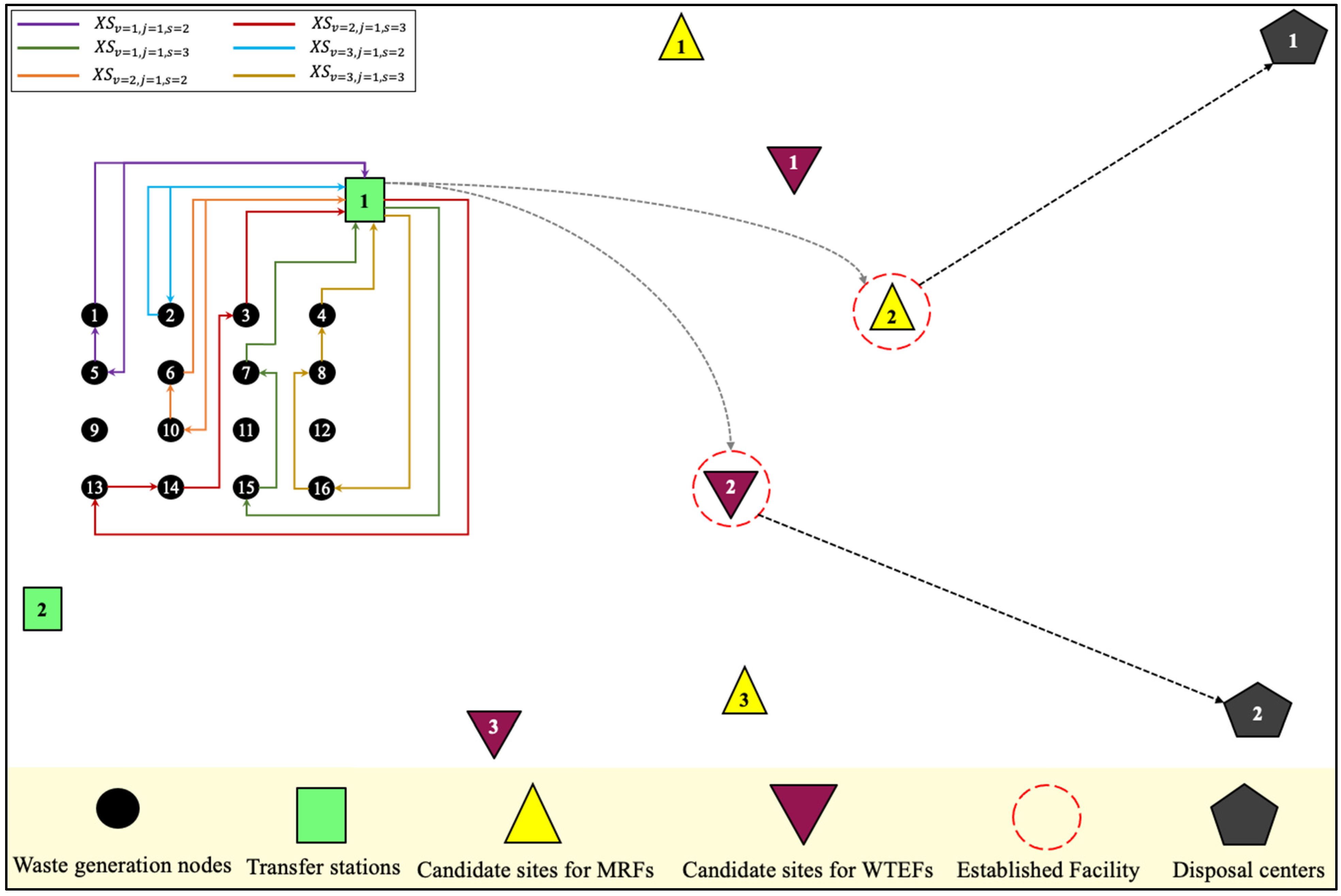
In this sub-section, the generated numerical experiments for the proposed WGP model are solved and their results are reported in

Table 6. Results obtained for the designed numerical experiments.

Problem No.	$\mathbf{Goal}\mathbf{Objective}\mathbf{Value}\left(\mathsf{\Gamma }\right)$	${\mathbf{D}}_1^{-}$	${\mathbf{D}}_2^{+}$	${\mathbf{D}}_3^{+}$	Gap (%)	Run Time (s)
1	0.164	0.000005	711,278.906	109.906	0	4.57
2	0.636	8.438	3,460,447.919	107.079	0	48.21
3	0.166	0.009	1,880,858.580	132.880	0	63.06
4	0.767	2.764	3,222,539.721	752.301	0	80.71
5	0.116	10.463	14,929.811	0.000	0	248.21
6	0.099	11.556	28,227.818	0.004	0	368.12
7	0.054	9.686	26,536.639	0.062	0	473.45
8	0.350	84.117	1,016,653.362	0.004	0	975.74
9	0.156	28.977	1,292,874.925	327.928	72.553	7212.48
10	767.967	68.282	2,402,044.160	10,520,819.556	99.975	7207.65

. According to the results obtained for Problems 1 to 8, the solver execution time is increased as the input size of the model increases. In these numerical examples, Gurobi could obtain the optimal solution for the integrated facility location, shift scheduling, and vehicle routing problem in the framework of the WGP model, and the optimality gaps between the best integer objectives and the objectives of the best nodes are zero. However, due to the complexity of the optimization model in the last two dimensions of the numerical examples (Problems 9 and 10), the Gurobi solver was unable to achieve the optimal solution within the 7200 s time limit considered in this study. In these two examples, the optimality gaps between the best-found solutions and the best node objectives are, respectively, 72.5 and 99.97 percent. Therefore, this reveals that the exact solution method cannot obtain an optimal or near-optimal solutions for medium- and large-scale problems within a reasonable amount of time, which is due to NP-hardness of the proposed integrated model. The obtained optimal solution for Problem 8 is presented schematically in Figure 2 as the largest numerical example solved optimally using the Gurobi solver. In the following sub-section, the sensitivity analysis on three parameters of the mathematical model is provided.

5.2. Sensitivity Analysis

To study the behavior of the optimization model, the sensitivity analysis is conducted with respect to the variations of three influential parameters including the WGP weighting coefficients, threshold waste level, and the importance level of social risk factors.

5.2.1. WGP Weighting Coefficients

In the goal programming approach, the weighting coefficients of the objective functions specify the priority or importance of the corresponding goals from the viewpoint of the DMs. The more priority given to objective function, the greater the weight that should be given to that goal. In this problem, three weighting coefficients determine the priority of objective functions. To evaluate the influence of weighting coefficients on the goal objective value and deviational variables, 33 scenarios are considered for the first numerical example (Problem 1). As shown in

Table A3. Sensitivity analysis results on the weighting coefficients of the WGP objective function.

${\mathbf{W}}_1$	${\mathbf{W}}_2$	${\mathbf{W}}_3$	$\mathbf{Goal}\mathbf{Objective}\mathbf{Value}\mathbf{\left(}\mathsf{\Gamma }\mathbf{\right)}$	${\mathbf{D}}_1^{-}$	${\mathbf{D}}_2^{+}$	${\mathbf{D}}_3^{+}$
0.00	0.50	0.50	0.000	10.178	4.859	0.000
0.10	0.45	0.45	0.052	3.569	3.072	0.000
0.20	0.40	0.40	0.102	3.348	24,392.132	0.000
0.30	0.35	0.35	0.150	3.348	24,397.109	0.000
0.40	0.30	0.30	0.148	0.000	711,278.906	109.906
0.50	0.25	0.25	0.734	0.000	6,532,705.797	109.906
0.60	0.20	0.20	0.116	0.220	686,878.650	109.993
0.70	0.15	0.15	0.453	0.000	6,736,309.031	109.906
0.80	0.10	0.10	0.327	0.000	7,337,445.456	109.906
0.90	0.05	0.05	0.214	0.000	9,718,025.190	109.906
1.00	0.00	0.00	0.000	0.000	711,278.000	31,936,604.000
0.50	0.00	0.50	0.097	0.000	711,276.000	109.906
0.45	0.10	0.45	0.130	0.186	711,277.643	109.906
0.40	0.20	0.40	0.151	0.220	711,277.938	109.972
0.35	0.30	0.35	0.158	0.000	711,278.906	109.906
0.30	0.40	0.30	0.150	3.348	24,397.109	0.000
0.25	0.50	0.25	0.127	3.348	24,394.620	0.000
0.20	0.60	0.20	0.103	3.432	12,359.447	0.000
0.15	0.70	0.15	0.078	3.569	0.000	0.000
0.10	0.80	0.10	0.052	3.569	0.000	0.001
0.05	0.90	0.05	0.026	3.569	0.000	0.001
0.00	1.00	0.00	0.000	3.569	0.000	8,141,266.000
0.50	0.50	0.00	0.149	0.000	711,273.917	11,207,197.000
0.45	0.45	0.10	0.154	0.000	711,278.906	109.906
0.40	0.40	0.20	0.158	0.000	711,278.906	109.906
0.35	0.35	0.30	0.163	0.000	711,276.583	109.906
0.30	0.30	0.40	0.149	3.348	24,393.844	0.000
0.25	0.25	0.50	0.866	0.693	7,084,868.751	109.906
0.20	0.20	0.60	68.785	3.432	818,482,326.706	0.000
0.15	0.15	0.70	0.078	3.569	0.000	0.102
0.10	0.10	0.80	44.888	3.534	1,068,593,693.864	0.000
0.05	0.05	0.90	13.570	3.432	645,638,317.735	0.000
0.00	0.00	1.00	0.000	10.042	12,361.000	0.000

(see Appendix B), the weights of the second and third objective functions are assumed equal in the first 11 cases, and the weight of the first objective is incremented by 0.1 unit, while the sum of all weights is equal to one. A similar approach is applied for the second and third objective functions in the next 22 cases. The results obtained from variations of the weighting parameters are reported in Table A3 and Figure 3. Figure 3a shows the influence of the first weighting coefficient (${\mathrm{W}}_1$) on the corresponding negative deviational variable (${\mathrm{D}}_1^{-}$) considered in the WGP model. Likewise, the effects of coefficients ${\mathrm{W}}_2$ and ${\mathrm{W}}_3$ on their corresponding postitive deviational variables (${\mathrm{D}}_2^{+}$ and ${\mathrm{D}}_3^{+}$) are, respectively, denoted in Figure 3b,c. According to the obtained results, by increasing the importance weight of an objective, the corresponding deviation from the predetermined goal is decreased aiming to satisfy the objective to the extent of its importance. According to the results in Table A3, the lowest weight coefficients in which the first, second, and third objective functions achieved the zero deviation from their corresponding goals are, respectively, 0.35, 0.7, and 0.15. The proposed LSR problem includes three conflicting objectives, and each combination of weight coefficients can achieve a specific balance between objective values. Thus, DMs and experts should prioritize conflicting objectives by determining the appropriate weight coefficients, to achieve the desired deviations from the goal values.

5.2.2. Threshold Waste Level

One of the factors that has a significant influence on the shift scheduling and vehicle routing decisions in the waste collection phase and, consequently, affect the sustainability of waste network is determination of threshold waste level for waste containers in a region or municipal area. The threshold waste level refers to the minimum level of waste containers (in percent) that requires the company to serve the corresponding containers. Obviously, the lower threshold level implies a higher number of containers that are collected. For example, in the 5 percent TWL, all containers whose waste levels are equal to or greater than the 5 percent of their capacities must be collected. In this sub-section, Problem 5 is considered as a sample numerical example and 10 distinctive levels of TWL are solved to assess the environmental impacts from the waste operations. The result obtained for each threshold level is presented in

Table A4. Sensitivity analysis results on the threshold waste level.

TWL for Waste Containers $\left(\mathsf{\gamma }\right)$	No. of Waste Generation Nodes Served in the Network $\left(\mathbf{\sum }_{\mathbf{i}\mathbf{\in }\mathbf{C}}{\mathbf{S}\mathbf{R}\mathbf{V}}_{\mathbf{i}}\right)$	Second Objective Function $\left({\mathbf{Z}}_2\right)$
5%	10	8,212,825.762
10%	9	8,096,152.325
20%	8	8,032,465.732
30%	7	7,785,312.569
40%	6	7,772,751.744
50%	5	7,178,956.432
60%	4	6,591,250.552
70%	3	5,764,037.103
80%	2	3,853,333.308
90%	1	2,442,048.636

and Figure 4. As expected, the higher threshold level in the waste collection phase leads to the lower number of containers that are served during the planning horizon. In addition, Figure 4 clearly shows that the emissions released by waste-related operations are significantly decreased considering higher TWLs. This, in turn, indicates that the transportation sector accounts for a substantial proportion of emissions released in the waste network activities. On the other hand, the collection of waste containers in the higher threshold levels might cause citizens dissatisfaction, due to aesthetic- or odor-related factors. Therefore, an appropriate TWL must be determined by the experts and DMs in a collection company to achieve a balance between all economic, environmental, and social factors.

5.2.3. Importance Level of Social Risk Factors

The other parameter that can considerably affect the policies in the proposed tri-objective optimization model is the importance level that prioritizes between the social-related goals in the third objective function, including the time window violations that imply the dissatisfaction of citizens, and the social risk factors originating from the establishment and operations of material recovery and waste-to-energy facilities. To investigate the sensitivity of the model to the importance level variations, Problem 3 is solved for a set of equally spaced values between 0.1 and 0.75. The behaviors of the goal objective and the third objective function are shown graphically in Figure 5, and the detailed results are presented in

Table A5. Sensitivity analysis results on the importance level of social risk factors.

$\mathbf{Importance}\mathbf{Level}\left(\mathsf{\theta }\right)$	$\mathbf{Third}\mathbf{Objective}\mathbf{Function}\left({\mathbf{Z}}_3\right)$	$\mathbf{Goal}\mathbf{Objective}\mathbf{Value}\left(\mathsf{\Gamma }\right)$
0.1	948.3784	0.119536
0.15	925.1275	0.119536
0.2	432.5035	0.119536
0.25	948.3784	0.119536
0.3	648.7552	0.119536
0.35	756.8809	0.119536
0.4	865.0069	0.119536
0.45	973.1328	0.128237
0.5	1081.2587	0.166241
0.55	1189.3845	0.204244
0.6	1297.5104	0.242248
0.65	1405.6363	0.280252
0.7	1513.7621	0.318256
0.75	1621.8880	0.356260

. In Figure 5, the horizontal axis depicts the importance level of the MRF- and WTEF-related social risk factors ($\mathsf{\theta }$) and, thus, the importance level of time window penalties is denoted by ($1-\mathsf{\theta }$) coefficient in the third objective function. According to the results obtained from different importance levels in Problem 3, the goal objective values and the social impacts in the third objective function are increasing steadily by selecting 0.45 or higher values of $\mathsf{\theta }$. As shown in Figure 5, considering the lower level of importance for the time window penalties (higher values of $\mathsf{\theta }$) can lead to higher deviations from goal values, social impacts, and dissatisfaction of citizens. Hence, it can be concluded that the dissatisfaction of citizens in receiving services within the predetermined time windows has a great impact on the social aspects of sustainability in the waste network. The evaluation of the model behavior by different combinations of importance levels enables DMs and responsible managers in the waste management companies to determine their most desirable policies. Accordingly, the satisfaction of citizens can be leveraged in all levels of the waste network along with optimizing the economic and environmental aspects of sustainability.

Finally, based on the analyses presented above, some managerial insights can be drawn as follows:

• Integrated Decision-Making: DMs must grasp the intricate dynamics of the waste management system by comprehending its economic, environmental, and societal impacts to assign the appropriate weight coefficients to each objective in the process. This nuanced understanding will guide the decisions made in waste management and help strike a balance among the competing objectives.
• Balanced Weight Coefficients: DMs need to balance the economic, environmental, and social implications when setting Time Window Limits (TWLs) for waste container collection. While diminishing emissions aligns with environmental sustainability, it should not negatively affect citizen satisfaction. The DMs must weigh the social repercussions of higher TWLs against their economic and environmental gains. Additionally, context-specific factors like population density, waste generation rates, and local regulations should be taken into account to ascertain the most suitable TWL for a specific area.
• Assessing Social Impact: Assessing the significance of social-related objectives when forming waste network policies is another crucial task for DMs. Despite the crucial nature of economic and environmental factors, social aspects of sustainability, such as citizen satisfaction, are equally important. The study’s findings suggest that, by assigning appropriate significance to social-related objectives, citizen satisfaction can be harnessed across all strata of the waste network. Furthermore, the proposed optimization model can be utilized by DMs to examine various combinations of significance levels to identify the most favorable policies. This approach allows for the optimization of the economic and environmental sustainability facets of the waste network, while concurrently ensuring citizen satisfaction.

6. Conclusions

This study presents a multi-objective mixed-integer linear programming model that aims to develop a unified framework for facility location, shift scheduling, and vehicle routing (LSR) within the context of efficient municipal solid waste management. The primary objective of this research was to integrate the three pillars of sustainability—economic profitability, environmental emissions, and social impacts, including citizen satisfaction—into a single comprehensive framework. To manage the model’s multi-objective nature, a weighted goal programming approach was employed. The model’s effectiveness and applicability were examined through a series of numerical experiments, designed using professional insights and customer input, and executed using the Gurobi solver in Python. Further, a sensitivity analysis was conducted on three significant parameters of the model—weight coefficient, threshold waste level, and social risk importance level—to explore their influence on the objectives.

The analysis results highlight the crucial role of transportation operations in the network’s gas emissions and demonstrate how the objectives deviate from goal values based on the weight coefficients assigned to conflicting objectives. It was also observed that different combinations of importance levels and policies significantly impact time window penalties and social risk factors, which, in turn, affect citizen satisfaction levels in and around the waste network. This research provides several key insights for management. The relative importance of each objective in the waste management process is paramount and demands a deep understanding of the system’s environmental, societal, and economic impacts. The balance between economic, environmental, and social factors when determining appropriate waste collection time windows is critical. Last, the importance levels assigned to social-related goals directly affect citizen satisfaction at all levels of the waste network.

While this study presents a robust framework for waste management, it also opens several avenues for future research, given its limitations. The proposed model’s complexity and NP-hardness necessitate the development of approximate solution methodologies, such as heuristics and meta-heuristic algorithms, for efficiently solving large-scale problems. Future studies could address the model’s realism by incorporating uncertainty factors using various approaches like fuzzy logic, two-stage stochastic programming, or distributionally robust optimization. Additionally, exploring other social factors affecting long-term citizen satisfaction from waste network operations could provide comparative insights into the study’s results.

References

- World Bank. Global Waste to Grow by 70 Percent by 2050 Unless Urgent Action Is Taken: World Bank Report. 2018. Available online: https://www.worldbank.org/en/news/press-release/2018/09/20/global-waste-to-grow-by-70-percent-by-2050-unless-urgent-action-is-taken-world-bank-report (accessed on 13 December 2021).
- Das, S.; Lee, S.H.; Kumar, P.; Kim, K.H.; Lee, S.S.; Bhattacharya, S.S. Solid waste management: Scope and the challenge of sustainability. J. Clean. Prod. 2019, 228, 658–678. [Google Scholar] [CrossRef]
- Breukelman, H.; Krikke, H.; Löhr, A. Failing Services on Urban Waste Management in Developing Countries: A Review on Symptoms, Diagnoses, and Interventions. Sustainability 2019, 11, 6977. [Google Scholar] [CrossRef] [Green Version]
- Tung, D.V.; Pinnoi, A. Vehicle routing–scheduling for waste collection in Hanoi. Eur. J. Oper. Res. 2000, 125, 449–468. [Google Scholar] [CrossRef]
- Hemmelmayr, V.; Doerner, K.F.; Hartl, R.F.; Rath, S. A heuristic solution method for node routing based solid waste collection problems. J. Heuristics 2013, 19, 129–156. [Google Scholar] [CrossRef] [Green Version]
- Zhang, A.; Venkatesh, V.G.; Liu, Y.; Wan, M.; Qu, T.; Huisingh, D. Barriers to smart waste management for a circular economy in China. J. Clean. Prod. 2019, 240, 118198. [Google Scholar] [CrossRef] [Green Version]
- Fan, X.; Zhu, M.; Zhang, X.; He, Q.; Rovetta, A. Solid waste collection optimization considering energy utilization for large city area. In Proceedings of the 2010 International Conference on Logistics Systems and Intelligent Management (ICLSIM), Harbin, China, 9–10 January 2010; pp. 1905–1909. [Google Scholar]
- Akhtar, M.; Hannan, M.A.; Begum, R.A.; Basri, H.; Scavino, E. Backtracking search algorithm in CVRP models for efficient solid waste collection and route optimization. Waste Manag. 2017, 61, 117–128. [Google Scholar] [CrossRef] [PubMed]
- Aringhieri, R.; Bruglieri, M.; Malucelli, F.; Nonato, M. An asymmetric vehicle routing problem arising in the collection and disposal of special waste. Electron. Notes Discret. Math. 2004, 17, 41–47. [Google Scholar] [CrossRef]
- Vonolfen, S.; Affenzeller, M.; Beham, A.; Wagner, S.; Lengauer, E. Simulation-based evolution of municipal glass-waste collection strategies utilizing electric trucks. In Proceedings of the 3rd IEEE International Symposium on Logistics and Industrial Informatics, Budapest, Hungary, 25–27 August 2011; pp. 177–182. [Google Scholar]
- Ramos, T.R.P.; Gomes, M.I.; Barbosa-Póvoa, A.P. Planning a sustainable reverse logistics system: Balancing costs with environmental and social concerns. Omega 2014, 48, 60–74. [Google Scholar] [CrossRef] [Green Version]
- Vidović, M.; Ratković, B.; Bjelić, N.; Popović, D. A two-echelon location-routing model for designing recycling logistics networks with profit: MILP and heuristic approach. Expert Syst. Appl. 2016, 51, 34–48. [Google Scholar] [CrossRef]
- Mirdar Harijani, A.; Mansour, S.; Karimi, B.; Lee, C.G. Multi-period sustainable and integrated recycling network for municipal solid waste—A case study in Tehran. J. Clean. Prod. 2017, 151, 96–108. [Google Scholar] [CrossRef]
- De Bruecker, P.; Beliën, J.; De Boeck, L.; De Jaeger, S.; Demeulemeester, E. A model enhancement approach for optimizing the integrated shift scheduling and vehicle routing problem in waste collection. Eur. J. Oper. Res. 2018, 266, 278–290. [Google Scholar] [CrossRef]
- Tirkolaee, E.B.; Mahdavi, I.; Mehdi Seyyed Esfahani, M. A robust periodic capacitated arc routing problem for urban waste collection considering drivers and crew’s working time. Waste Manag. 2018, 76, 138–146. [Google Scholar] [CrossRef] [PubMed]
- Erdinç, O.; Yetilmezsoy, K.; Erenoğlu, A.K.; Erdinç, O. Route optimization of an electric garbage truck fleet for sustainable environmental and energy management. J. Clean. Prod. 2019, 234, 1275–1286. [Google Scholar] [CrossRef]
- Tirkolaee, E.B.; Mahdavi, I.; Esfahani, M.M.S.; Weber, G.W. A robust green location-allocation-inventory problem to design an urban waste management system under uncertainty. Waste Manag. 2020, 102, 340–350. [Google Scholar] [CrossRef] [PubMed]
- Ghannadpour, S.F.; Zandieh, F.; Esmaeili, F. Optimizing triple bottom-line objectives for sustainable health-care waste collection and routing by a self-adaptive evolutionary algorithm: A case study from tehran province in Iran. J. Clean. Prod. 2021, 287, 125010. [Google Scholar] [CrossRef]
- Anagnostopoulos, T.; Kolomvatsos, K.; Anagnostopoulos, C.; Zaslavsky, A.; Hadjiefthymiades, S. Assessing dynamic models for high priority waste collection in smart cities. J. Syst. Softw. 2015, 110, 178–192. [Google Scholar] [CrossRef] [Green Version]
- Salehi-Amiri, A.; Akbapour, N.; Hajiaghaei-Keshteli, M.; Gajpal, Y.; Jabbarzadeh, A. Designing an effective two-stage, sustainable, and IoT based waste management system. Renew. Sustain. Energy Rev. 2022, 157, 112031. [Google Scholar] [CrossRef]
- Jatinkumar Shah, P.; Anagnostopoulos, T.; Zaslavsky, A.; Behdad, S. A stochastic optimization framework for planning of waste collection and value recovery operations in smart and sustainable cities. Waste Manag. 2018, 78, 104–114. [Google Scholar] [CrossRef] [PubMed]
- Charnes, A.; Cooper, W.W.; Ferguson, R.O. Optimal Estimation of Executive Compensation by Linear Programming. Manag. Sci. 1955, 1, 138–151. [Google Scholar] [CrossRef]
- Gurobi Optimizer. Available online: https://www.gurobi.com/products/gurobi-optimizer/ (accessed on 21 August 2022).
Figure 1.
Framework of the multi-echelon municipal solid waste network.
Figure 2.
Optimal solution obtained by Gurobi solver for Problem 8 of the numerical examples.
Figure 3.
The effect of variations in the weighting coefficients on their corresponding deviational variables. (a–c) effects of coefficients and on their corresponding postitive deviational variables ( and ) are, respectively.
Figure 4.
The effect of threshold waste level () on the second objective function ().
Figure 5.
The effect of importance level () on the goal objective () and third objective function ().