
More Than Half of Emitted Black Carbon Is Missing in Marine Sediments

1
Environment Research Institute, Shandong University, Qingdao 266237, China
2
Laboratory for Marine Geology, Qingdao National Laboratory for Marine Science and Technology, Qingdao 266061, China
3
Collaborative Innovation Center of Climate Change, Nanjing 210023, China
4
CSIR—National Institute of Oceanography, Panaji 403004, India
5
Yantai Environmental Monitoring Center, Yantai 264003, China
6
Key Laboratory of Marine Geology and Metallogeny, First Institute of Oceanography, Ministry of Natural Resources, Qingdao 266061, China
*
Author to whom correspondence should be addressed.
Sustainability 2023, 15(12), 9739; https://doi.org/10.3390/su15129739
Submission received: 31 March 2023
/
Revised: 22 May 2023
/
Accepted: 6 June 2023
/
Published: 19 June 2023
(This article belongs to the Special Issue Characteristics, Sources, and Impacts of Black Carbon Aerosols)
Abstract
:Marine sediments are the ultimate reservoir for black carbon (BC) preservation, and BC burial in sediment/soils is an efficient method for carbon sequestration to mitigate CO2 emissions. A portion of soil charcoal and atmospheric BC is dissolved in inland and oceanic water, but the amount of BC in the ocean remains unclear. We analyzed multi-sediment cores from the northwestern Pacific Ocean and lakes in China and reconstructed the timeline of BC deposition from 1860 to ~2012. The lacustrine sediment cores showed an increase in BC deposition by a factor of 4–7 during the industrialization period in China compared to the years 1860–1950 (reference level). Such increasing trends in BC have also been reproduced by ten global climate model simulations. However, the marine sediment cores did not retain these significant increases in BC deposition. Meanwhile, the model simulations predicted increased trends compared to the observed flat trends of BC deposition in marine sediments. The discrepancy suggests a large amount of BC, i.e., 65 (±11)%, is missing in marine sediment sinks. Thus, since more than half of emitted BC has dissolved into oceanic water, the dissolved BC and carbon cycle should be reconsidered in the global carbon budget.
1. Introduction
Black carbon (BC) is one of the most crucial atmospheric pollutants and plays a vital role in global climate change and biogeochemical cycles [1]. It is predominantly composed of fine particles (<2.5 µm), which are mainly emitted into the atmosphere through the incomplete combustion of fossil fuel and biomass [2,3,4,5,6]. Due to its long atmospheric lifetime (from a few days to weeks), it can travel over a large distance through long-range transportation from one continent to another before wet/dry deposition [7,8,9,10]. It has recognition as a key global warming pollutant, having the second-largest contribution to global climate warming after carbon dioxide [1,5]. Marine sediments are unique sinks for BC via atmospheric deposition and riverine transports. Due to its refractory nature, the BC in sediments can be used as a proxy for pollution levels, and the dating of temporal BC becomes a useful diagnostic tool helping us to understand recent and past emission sources, energy demands and past environmental changes [11,12,13,14]. Soil is one of the major reservoirs of BC, where it can be stored it for up to several centuries before it enters the ocean through riverine discharges [15]. Earlier studies suggest that riverine exports and atmospheric deposition are the two major processes through which BC reaches the ocean [12,16,17,18,19,20]. An earlier study also reported a large portion of BC is exported to the ocean in the form of dissolved black carbon (DBC), i.e., ~27 Tg yr−1 [18]. However, Jones et al. [21] reported a relatively lower contribution of riverine discharge of DBC into the global ocean, i.e., ~18 ± 4 Tg yr−1, though this is still significantly high in comparison to the atmospheric deposition of DBC, i.e., 1.8 ± 0.83 Tg yr−1 [22]. An earlier study also reported that nearly 208 ± 28 Tg yr−1 dissolved organic carbon (DOC) is exported into the global oceans through riverine discharges [23], and nearly 10% of this DOC is found in the form of DBC, showing a strong linear relationship between DBC and DOC [14,17,24]. The positive correlation between DBC and DOC is mainly due to the similar environmental control factors seen during the mobilization process of soil black carbon and organic carbon [21]. In another study, Jaffe et al. [24] found that ~26 Tg yr−1 DBC is deposited into the ocean, which is mainly due to the dissolution of charcoal into the ocean in the form of soils travelling through rivers. Recently, BC in the marine carbon cycle has received significant attention among the global scientific community, since a significant amount (nearly 10% of the total oceanic bulk dissolved organic carbon pool) of BC is found in the form of DBC [12,17,25]. Earlier studies also show a loss of significant fractions of total oceanic BC via various processes, such as photo-oxidation, dissolution, and subsequent transport to the ocean, resulting in a very small fraction of BC that reaches the bottom of the abyssal zone through lateral transport in the water column and is preserved in the form of marine sediments [22,24]. Thus, a small fraction of total BC is preserved in marine sediments due to the loss of a significant portion of atmospheric BC via dissolution and subsequent transport to the ocean. However, direct estimation of the amount of BC present in the ocean is very difficult [22,24]. The transportation of BC from the land/atmosphere to the ocean is an important constraint on the global CO2 cycle because of its residence time (up to many centuries) in sea sediments. Therefore, the transportation of BC in the form of DBC and particulate BC (PBC) to inland, coastal, and oceanic waters is associated with large uncertainty and needs to be addressed more accurately in global geochemical models [17].
During the last century, China has witnessed a large increase in BC emissions (approximately 25% of the global BC emissions) mainly because of rapid urbanization/industrialization, economic development, and the associated energy demands [11,26,27,28], which has lead to an overall trend of increasing BC [29,30]. North China Plain (NCP) provinces (such as Beijing, Tianjin, Hebei, and Shandong) have the strongest BC emission intensity, contributing ~36% to the total BC emissions of China in 2006 [29]. This emitted BC is deposited on adjacent continental shelves in the ocean through various processes, such as riverine outflow, atmospheric deposition, etc., and can reach the northwestern Pacific Ocean region through downwind flow [7,22]. Thus, the northwestern Pacific Ocean region could be a good reservoir for BC and has vital importance in research attempting to understand the BC transport pattern along with the global carbon cycle [14,31,32]. The estimation of BC flux and DBC concentration will be helpful to policymakers for the improvement in environmental pollution mitigation strategies [33,34] as well as for accurate parameterization of global climate models [35].
In the present study, we analyzed BC concentrations along with BC fluxes in multi-sediment cores from the northwestern Pacific Ocean (including the East China Sea and Sea of Japan) and lakes spanning from the north to south of China. BC flux was also simulated using ten models from the Coupled Model Intercomparison Project Phase 5 (CMIP5). We compared BC flux differences between lacustrine and marine deposition and estimated the loss of BC in marine sediments, which will be helpful to accurately estimate the global amount of BC.
2. Materials and Methods
2.1. Sediment Core and Dating
The details of the sampling locations for sediment cores studied in the present study and other pertinent information are presented in Figure 1a and Table 1. In brief, samples from three sediment cores in the Sea of Japan (Figure 1a; Table 1) were collected using gravity corers during a joint research campaign by the First Institute of Oceanography Marine Science and Numerical Modeling, Pacific Ocean Institute, Far East Branch, and the Russian Academy of Sciences in November 2010. The core samples were cut onboard the research vessels into sections of 1 or 2 cm down the core length with a stainless-steel cutter. The collected sediment slices were packed in aluminum foil (combusted at 450 °C for 4 h before use) and stored at −20 °C until further analysis. Additionally, three other sediment cores, S4, S5, and S8, were taken from a wild marsh in the south of Tianjin (Table 1). Cores S4 and S5 were sampled at an interval of 1 cm for 1 m deep sediments; however, S8, a parallel sample of S4, was collected with 0.5 cm interval sampling. These cores represent the major emission source areas in East Asia and outflow pathways of BC and other air pollutants in the northwestern Pacific Ocean [22]. The ages of the S4 and S5 samples were determined via radio isotope dating for 210Pb and 137Cs, which is a widely used and well-accepted method worldwide [2,13,36,37]. The age of S8 was calibrated from S4’s age profile since the two cores were parallel samples with very similar sedimentation environments. The sedimentation rates were estimated based on the excess 210Pb (210Pbexc) and 137Cs in the sediment [38] using the CIC age model. The values for both 210Pbexc and 137Cs suggested that there was no sediment mixing layer and no erosion in the upper half of the S4 (S8) and S5 cores [11]. Apart from these samples, sediment cores from the East China Sea [13] and two lakes (Lake Chaohu and Lake Huguangyan) in China [37] were also re-analyzed in the present study (Table 1).
2.2. Quantification of Sedimentary BC
In the present study, we adopted acid pretreatment integrated with the thermal optical reflectance (TOR) method to quantify BC concentrations (in mg g−1). This method thermally discriminates between organic carbon (OC) and BC. Before acid pretreatment, the sediment samples were freeze-dried and finely ground (<63 μm). A 0.1 g sample was digested with HCl (2 mol) acid for 24 h at room temperature to eliminate carbonates and some metals. The remaining residues were further digested with HF acid (2 mL) for the next 24 h at room temperature to remove any superficial carbonaceous materials that may have been trapped between the silicate sheets. Again, the remaining residues were digested with HCl for 24 h at room temperature to remove minerals such as fluorite. The remaining residues were filtered through a 47 mm quartz filter, which had been pre-combusted for 6 h at 600 °C. The carbonate-free filter samples were air-dried for BC analysis. Subsequently, the quartz filters were analyzed for BC using a Sunset carbon analyzer (Sunset Laboratory, Tigard, OR, USA) following a high-temperature protocol (Interagency Monitoring of PROtected Visual Environment: IMPROVE–H). In this protocol, the sample filter was heated in a progressive manner to 140 °C, 280 °C, 480 °C, and 580 °C in a pure helium environment, which produced four organic fractions (OC1, OC2, OC3, and OC4). After that, the temperature was further raised to 580 °C, 740 °C, and 840 °C in an oxygen–helium (2:98 v/v) atmosphere, which provided the three elemental carbon fractions (EC1, EC2, and EC3). Further details about the analytical procedures are discussed elsewhere [7,11,13,31]. We selected 10% random samples and performed repeat measurements to ensure reproducibility. The relative standard deviation (RSD) from duplicate analyses was found to be within 0–10%, while the average was 4.66%. In addition to this, we also analyzed blanks and seven National Institute of Standards and Technology standard reference materials (NIST SRM-1941b, marine sediments collected from Baltimore Harbor, Baltimore, MD, USA). The BC content in NIST SRM-1941b was found to be 9.66 ± 0.79 mg g−1, which is very close (up to 10% deviation) to the results reported by previous studies [8,13,31,39,40] (Table S1).
2.3. Estimation of BC Fluxes
BC flux is a more reliable measurement than the concentration of sedimentary BC because fluxes are not affected by the dilution or concentration effect of minerals and organic matter [11,41,42]. The BC flux was estimated as follows:
where FBC is the burial flux (g m−2 yr−1), BC is the black carbon concentration (mg g−1) in the sediment sample, and ω is the sediment mass accumulation rate (MAR: in g cm−2 yr−1), which is dependent on sediment properties, including the dry bulk density (DBD: g cm−3) of the sediment sample, sediment porosity (dimensionless), and sedimentation rate (S: in cm yr−1). The MAR (ω) of sediment samples was calculated as follows:
FBC = BC (mg g−1) × ω
ω (g cm−2 yr−1) = DBD (g cm−3) × S (cm yr−1)
The sedimentation rate (S) of the sediment sample was calculated using the CIC model with a given equation:
where D is the depth to z (cm), and C0 and C are the activity of the top layer of sediment and the activity of sediment at the z layer, respectively. λ is the decay constant (0.031 yr−1) for 210Pb [37]. Further details about the BC flux calculation are discussed in an earlier study [11]. To investigate the impact of anthropogenic emissions and industrialization on BC emissions, the increase factor (IF) of BC fluxes for each period was calculated using the reference period of 1860–1950 (i.e., the ratio of BC fluxes in each time period to BC fluxes during the time period of 1860–1950). Higher IF values represent higher BC flux changes during the particular period of 1860–1950.
S (cm yr−1) = λ D/ln (C0/C)
2.4. Simulation of Historical BC
The Coupled Model Intercomparison Project Phase 5 (CMIP5) is a series of coordinated climate model experiments by twenty different climate modeling groups from all around the world [39], and the simulation results are discussed in the Fifth Assessment Report (AR5) of the Intergovernmental Panel on Climate Change (IPCC). A majority of CMIP5 models simulate the concentrations of different types of aerosol species, i.e., dust, sea salt, nitrate, sulfate, particulate organic matter, and black carbon, and are used to examine the aerosol drivers of climate change [43]. In this study, ten CMIP5 climate models with BC simulations for the twentieth century and projections for the twenty-first century were used [44,45,46,47,48,49,50,51,52,53] (Table S2). The simulations included interactive chemistry, aerosols, and dust driven by emissions and have the same emission inventories of anthropogenic BC, organic carbon (OC), and SO2 [54,55,56]. A brief description of the climate models used in BC simulation is discussed in the Supplementary Materials.
2.5. BC Emission Inventory and Global Precipitation
The available BC emission data (1960–2012) from wildfire and agricultural burning for the summer (JJA: June, July, August) and winter seasons (DJF: December, January, February) were retrieved from the emission inventory of the Department of Environmental Science, Peking University (PKU; http://inventory.pku.edu.cn/home.html, accessed on 30 March 2023). The available precipitation data (1979–2012) for the summer and winter seasons were retrieved from the Global Precipitation Climatology Project (GPCP) version 2.3 (http://gpcp.umd.edu/, accessed on 30 March 2023). Further details about the emission inventory and precipitation data are described elsewhere [29,57].
3. Results and Discussion
3.1. Trends of Sedimentary BC Fluxes in Continental and Marine Sediment Cores
BC fluxes were calculated for all the sediment cores, and are given in Tables S3–S6 for the sediment cores from the Sea of Japan, the East China Sea, south Tianjin, and Lake Chaohu and Lake Huguangyan, respectively. The mean BC flux in the Sea of Japan ranged between 1.31 and 2.41 g m−2 yr−1, while a relatively higher value of BC fluxes was found for the sediments from the East China Sea with a wide range from 1.4 to 12.6 g m−2 yr−1. The higher value of BC fluxes over the East China Sea suggests relatively higher BC deposition through different atmospheric processes. Earlier studies also reported a higher concentration of BC near the coastal region of the East China Sea [10,13,31,33]. On the other hand, the BC fluxes found for the Tianjin sediment core were in the range of 1.5–2.5 g m−2 yr−1, which is about 2 to 8 times higher than the BC fluxes found for the lake sediments (0.74 g m−2 yr−1 and 0.32 g m−2 yr−1 for Lake Chaohu and Lake Huguangyan, respectively). The higher value of BC flux for Tianjin sediments was mainly attributed to the industrial development and rapid urbanization in this region during the last few decades, which caused huge amounts of atmospheric pollutant emissions, including BC [11,58]. The spatial variations in BC emissions and atmospheric BC concentrations also show relatively higher values in eastern China and the coastal region of the marginal sea, including Tianjin, Nanjing, and Shanghai, compared to the rest of mainland China (Figure 1a,b).
BC fluxes for all sediment cores showed a large temporal variation with an increasing trend of different magnitudes (Figure S1) [59,60,61,62,63,64], mainly because of the technological developments in energy sources during the last century [13]. The implementation of various emission control policies from different authorities might also have had a significant contribution to the decline in BC emissions and other pollutants for certain intervals (Figure S1) [58]. The BC fluxes along with their standard deviation (SD) and IF for four different time periods are given in Table 2. In detail, during the pre-industrial age (1860–1950) in China, all the sediment cores showed nearly constant trends of BC fluxes. After that, the BC fluxes rapidly increased, which is more prominent for the continental sediment cores. The observed results were further confirmed with CMIP5 simulations (Figure S2). The average BC flux in the Tianjin cores increased from 0.6 ± 0.4 (1860–1950) to 1.6 ± 0.9 g m−2 yr−1 during 1980–2000 and reached 4.5 ± 2.2 g m−2 yr−1 in 2000–2012 (Figure 1c). Similar increasing trends were also identified from 1860–1950 to 2000–2012 in the Lake Chaohu cores (0.3 ± 0.1, 1.0 ± 0.3, and 1.3 ± 0.2 g m−2 yr−1) and Lake Huguangyan cores (0.11 ± 0.02, 0.45 ± 0.03, 0.59 ± 0.08 g m−2 yr−1). Compared to the 1860–1950 levels, the average BC fluxes increased by a factor of 7.7, 4.7, and 5.6 for the sediment cores from Tianjin, Lake Chaohu, and Lake Huguangyan, respectively, for the time period of 2000–2012 (Table 2). Earlier studies reported a sharp increase in BC concentrations and other pollutants in the Tianjin region [11,59,60,65]. Recently, Neupane [2] also found an increasing trend of BC fluxes in the four lake sediments of the Tibetan Plateau, i.e., Ranwu (6.42 ± 2.61 g m−2 yr−1), Qiangyong (1.37 ± 0.26 g m−2 yr−1), Tangla (0.39 ± 0.10 g m−2 yr−1), and Lingge Co (0.06 ± 0.03 g m−2 yr−1). In another study, Cong et al. [8] reported a very similar trend of increasing BC flux in the sediment of Nam Co Lake (average BC flux: 0.26 g m−2 yr−1).
On the other hand, a moderate increase in BC fluxes was recorded in the marine sediment cores. The average BC fluxes in the marginal sea were found to be between 1.4 and 9.2 g m−2 yr−1 during 1860–1950, demonstrating an increase factor of up to 2.3, and the fluxes reached between 1.8 and 20.8 g m−2 yr−1 in 2000–2012 (Table 2 and Figure 1c). Among all the studied marine sediment cores, the East China Sea core had the highest BC flux. However, the increase in BC flux from 1860–1950 to 2000–2012 was very similar for both the East China Sea (2.3) and the Bohai Sea (2.1), indicating similar industrial developments near both regions. Recent studies also reported higher BC concentrations in the sediment of the Bohai Sea and East China Sea [13,31].
3.2. Sediment Cores and Simulations
To validate the BC trends in sediment cores, simulations of atmospheric BC fluxes from CMIP5 were retrieved for ten General Circulation Models (GCMs) with historical BC deposition fluxes (Table S2). These GCMs predict that both marine (Figure 2b) and continental (Figure 2d) sediment cores will show a comparatively rapid increase in BC deposition since 1950. For the continental cores from China, the average BC fluxes for 2000–2012 increased nearly 4–7 times compared to the pre-industrial period. This increase in BC flux suggests an increase in BC emissions and deposition during the industrialization period, which was further confirmed by the GCM simulations. However, the GCM results also support a relatively lower increase factor in marginal sea sediment than the continental sediment (Figure 2b,d), which may be because of the ocean currents, which can impact BC deposition fluxes and could be one of the possible reasons for the discrepancy in BC fluxes between marine sediment cores and GCM simulations. Earlier studies also suggest that a strong ocean current has significant energy and is capable of transporting coastal sediments to the open ocean [66,67]. However, the impact of ocean currents should be offset in GCM simulation by using as an increase factor the ratio of BC fluxes between the two time periods. Compared to the average BC flux for the period of 1860–1950, the BC fluxes for 1980–2000 were increased by a factor of 1.2, 1.1, 1.5, and 1.4 in the Bohai Sea, Yellow Sea, East China Sea, and Sea of Japan, respectively (Figure 2a), and the increases were relatively lower than those for 2000–2012 (2.1, 1.4, 2.3, and 1.3). The increasing trend of BC was much lower in sea sediments than the continental sediment cores from China (Figure 2c), which suggests some loss of BC in to the ocean through various processes, such as photo degradation or water column export to the abyssal zone.
3.3. Spatial Variations and Simulations
The spatial variations in BC concentration and their fluxes provide valuable information about the impact of anthropogenic emissions on global as well as regional climate change [5,68]. Therefore, the spatial variation in BC concentration for the sediment cores was derived from ten different CMIP5 model simulations (Table S2). The simulated BC concentration was quite consistent with the observed BC concentration during the summer season (Figure S3) [69]; however, it was slightly underestimated in urban hotspots during the winter season (Figure S4). For all ten models, GISS model simulation was very close to the central estimates of the model ensembles. Since the sediment core profiles were too sparse to interpolate the spatial variations in BC fluxes, we computed the BC increase factor (IF) from surface sediment samples used by earlier studies [31,41]. A positive correlation (R2 = 0.66) between BC increase factors and BC fluxes was found (Figure 3a), which can be fitted with a linear regression given by
where x is the surface BC flux, and y stands for the BC increase factor. The average spatial variation in BC increase factors for the 2000–2012 interval was predicted using a model (GISS) (Figure 3b). Then, the spatial variations in the BC increase factor for the Bohai Sea and Yellow Sea (Figure 3d) were derived from surface sediment BC fluxes (Figure 3c) in compliance with the regression. These surface sediment BC increase factors are consistent with core results and in the range of 1~2, with higher values in the Bohai Sea and coastal areas. Although such a spatial trend is compatible with model predictions, the values are significantly lower than the predictions (Figure 3b). Earlier studies also reported an increase in BC flux in the sediments of the Bohai Sea and the Yellow Sea during the last two decades [13,31].
y = 0.048x + 1.1846
3.4. BC Missing in Marine Sediments
Both marine sediment cores and surface sediment revealed a significant absence of BC deposition. The modeling of BC increase factors suggests a large fraction of BC, i.e., 67 (±11)%, 72 (±6)%, 63 (±5)%, and 55 (±17)%, is missing from the marine sediments of the Bohai Sea, Yellow Sea, East China Sea, and the Sea of Japan, respectively (Table 3). The average missing fraction of BC was found to be 65 (±11)% in the northwestern Pacific Ocean. Such a large amount of missing BC might be attributed to the fraction dissolving into the aquatic system, which is known as DBC or unknown BC/carbon pool in the ocean. The oxidation of freshly emitted BC from combustion sources enhances its water solubility and potentially makes it one of the major sources of DBC in the ocean [70]. Riverine discharge (mostly from the Yellow River) is another way in which BC is dissolved and deposited into the adjacent ocean of mainland China. A recent study reported that the Yellow River alone contributed around 37% and 32% of total DBC exports (16.3 and 6.4 Gg yr−1) to the Bohai Sea during 2013 and 2014, respectively [14]. The DBC from riverine discharge is mainly derived from the stocks of charcoal stored in the soils of river catchments [17] and fine aerosols (soot) deposited from the atmosphere to river catchments [16,71]. It is reported that the global flux of soluble charcoal accounts for 26.5 ± 1.8 million tons per year, of which 11~66% may be produced by global biomass burning [24]. Studies have reported a good correlation between DBC and DOC concentrations, which suggests that they are exported in a coupled manner in various environmental conditions [12,14,17,24].
On the other hand, biomass burning is another substantial source of BC (up to 27% of total BC), and nearly 90% of the global burned area is in the tropics [18,22,72]. The spatial variation in biomass burning from wildfire and agriculture along with monthly mean total precipitation for three different time spans, i.e., 1960–1980, 1981–2000, and 2001–2012, is given in Figure S5 (for summer) and Figure S6 (for winter). The figures reflect a large increase in biomass burning (from both wildfire and agriculture) from 1960 to 1980 for both seasons. An increase in BC emissions causes a reduction in precipitation, suggesting that emission variations play a major role in the changes in the deposition of these fine particles into the ocean via wet deposition. A recent study also suggests a significant amount of water-soluble BC (WSBC), i.e., 0.072 ± 0.042 Ggd−1, is deposited into the Yellow Sea and the East China Sea through dry deposition [22]. Apart from this, the concentration of DBC in the ocean also depends on the PBC deposition rate, which influences the DBC fluxes [16,24,73]. Thus, the transportation of BC from the land to the ocean could be a major constraint on the global BC budget because this extends the lifetime of BC across several decades [18,73,74,75]. The decrease in BC deposition to marine sediment constrains the upper limit of the soluble fraction, and hence the DBC budget may play a much more important role in BC emissions and the carbon cycle than previously thought. More than half of emitted BC may be dissolved into the ocean, which directly/indirectly affects oceanic productivity through different cycling paths.
4. Conclusions
In the last few decades, rapid urbanization, economic development, and the associated energy demands have caused intense BC emissions from China (particularly the North China Plain and coastal region of China) to be deposited into the adjacent ocean through various processes. Our results suggest that the marginal East China Sea has the highest BC flux, which is also supported by simulated atmospheric BC concentrations. A large temporal variation in BC flux for all sediments was found, which could be due to the implementation of various emission control policies. An overall increasing trend in BC flux was found for all studied cores and was more prominent for the pre-industrial age (i.e., 1860–1950).
Interestingly, the increase in BC flux in marine sediment cores from 1860–1950 to 2000–2012 was found to be very similar for the East China Sea (IF: 2.3) and Bohai Sea (2.1), while for the continental cores from China, it was found to be ~4–7 times higher. These results were further confirmed with CMIP5 simulations. A large difference in the IF was found between sea sediments and continental sediment cores, suggesting the loss of black carbon into the ocean through different pathways, such as photodegradation, water column export, etc., which need to be studied meticulously. The present study concludes that a significant amount (i.e., 65 (±11)%) of BC is deposited in marine sediments in the form of dissolved BC. Thus, the DBC budget may play a vital role in BC emissions and carbon cycle and must be reconsidered in the global carbon budget.
Supplementary Materials
The following supporting information can be downloaded at: https://www.mdpi.com/article/10.3390/su15129739/s1, Table S1: Summary of measurements of marine sediment standard of NIST SRM-1941b; Table S2: The models for the simulations of BC in Climate Model Intercomparison Project Phase 5 (CMIP5) along with model description; Table S3: History of BC fluxes for the three sediment cores from the Sea of Japan (SJP); Table S4: BC fluxes (g m−2 yr−1) for sediment cores from the Bohai Sea, Yellow Sea (NYS and SYS), and East China Sea (ECS1 and ECS2); Table S5: BC fluxes for the three sediment cores from south Tianjin; Table S6: The 150-year history of BC fluxes for sediment cores from Lake Chaohu and Lake Huguangyan (Huguangyan Maar Lake). Figure S1: Trends of sediment BC fluxes (a–e) and BC emission inventories (f); Figure S2: BC fluxes of measured sediment cores and simulated atmospheric deposition. The models show the simulations (1–99 percentile ranges) and median value. (a–d) are marine sediment cores from the northwestern Pacific Ocean, while (e,f) are lake sediment cores from China; Figure S3: observations and simulations of black carbon aerosol emissions in summer. Observations are shown for urban and rural areas in China. The simulations from ten models of CMIP5 (Table S2) are shown as panels with shading patterns. Black carbon observations were reviewed from recent publications in China; Figure S4: Similar to Figure S3 but for the winter season; Figure S5: Spatial variation in Peking University (PKU) Inventory-derived BC emissions (g, BC/km2 month) from wildfire (upper panel) and agriculture (middle panel) along with monthly mean precipitation (mm/day) (lowest panel) obtained from the Global Precipitation Climatology Project (GPCP) version 2.3 during summer (JJA) for the three different time scales, i.e., 1960–1980, 1981–2000, and 2001–2012 for BC and 1979–1980, 1981–2000, and 2001–2012 for precipitation; Figure S6: Similar to Figure S5 but for the winter (DJF) season. References [76,77,78,79,80,81] are cited in Supplementary Materials.
Author Contributions
Conceptualization, B.C. and S.T.; methodology, B.C., S.T. and J.Z.; formal analysis, B.C., S.T. and K.L.; resources, B.C. and J.Z.; data curation, S.T. and K.L.; writing—original draft preparation, B.C. and S.T.; writing—review and editing, B.C. and S.T.; project administration, B.C.; funding acquisition, B.C. All authors have read and agreed to the published version of the manuscript.
Funding
This research was funded by the Key Research and Development Program of Shandong Province (2017GHY215005), Laboratory for Marine Geology, Qingdao National Laboratory for Marine Science and Technology (grant no. MGQNLM-KF201703), and the Taishan Scholars (no. ts201712003).
Institutional Review Board Statement
Not applicable.
Informed Consent Statement
Not applicable.
Data Availability Statement
The data in this study are available on request from the authors.
Acknowledgments
Yongming Han and his group kindly offered their help for sedimentary BC measurements. Yin Fang provided useful suggestions. This research received funding from the Science and Technology Project of Laoshan Laboratory (grant no. LSKJ202204203), Key Research and Development Program of Shandong Province (2017GHY215005), Laboratory for Marine Geology, Qingdao National Laboratory for Marine Science and Technology (grant no. MGQNLM-KF201703), and the Taishan Scholars (no. ts201712003). One of the authors, Shani Tiwari, is thankful to Shandong University, China, for the financial support provided under the International Postdoctoral Exchange Program. We acknowledge the use of freely available CMIP5 models output data, which can be obtained via the ESGF peer-to-peer enterprise system site (https://esgf-node.llnl.gov/search/cmip5/, accessed on 30 March 2023), Peking University (PKU) inventory data (http://inventory.pku.edu.cn/download/download.html, accessed on 30 March 2023), and Global Precipitation Climatology Project (GPCP) version 2.3 data (https://www.esrl.noaa.gov/psd/data/gridded/data.gpcp.html, accessed on 30 March 2023). All the data reported in this study can be found in the supporting information file, tables, and references associated with this manuscript. We are also thankful to both anonymous reviewers for their constructive comments/suggestions, which certainly helped us to improve the content of this manuscript.
Conflicts of Interest
The authors declare no conflict of interest.
References
- Ramanathan, V.; Carmichael, G. Global and regional climate changes due to black carbon. Nat. Geosci. 2008, 1, 221–227. [Google Scholar] [CrossRef]
- Neupane, B.; Kang, S.; Chen, P.; Zhang, Y.; Ram, K.; Rupakheti, D.; Tripathee, L.; Sharma, C.M.; Cong, Z.; Li, C.; et al. Historical Black Carbon Reconstruction from the Lake Sediments of the Himalayan-Tibetan Plateau. Environ. Sci. Technol. 2019, 53, 5641–5651. [Google Scholar] [CrossRef] [PubMed]
- Ruppel, M.M.; Gustafsson, Ö.; Rose, N.L.; Pesonen, A.; Yang, H.; Weckström, J.; Palonen, V.; Oinonen, M.J.; Korhola, A. Spatial and Temporal Patterns in Black Carbon Deposition to Dated Fennoscandian Arctic Lake Sediments from 1830 to 2010. Environ. Sci. Technol. 2015, 49, 13954–13963. [Google Scholar] [CrossRef]
- Coppola, A.I.; Ziolkowski, L.A.; Masiello, C.A.; Druffel, E.R.M. Aged black carbon in marine sediments and sinking particles. Geophys. Res. Lett. 2014, 41, 2427–2433. [Google Scholar] [CrossRef] [Green Version]
- Bond, T.C.; Doherty, S.J.; Fahey, D.W.; Forster, P.M.; Berntsen, T.; Deangelo, B.J.; Flanner, M.G.; Ghan, S.; Kärcher, B.; Koch, D.; et al. Bounding the role of black carbon in the climate system: A scientific assessment. J. Geophys. Res. Atmos. 2013, 118, 5380–5552. [Google Scholar] [CrossRef]
- Zhang, X.; Zhu, Z.; Cao, F.; Tiwari, S.; Chen, B. Source apportionment of absorption enhancement of black carbon in different environments of China. Sci. Total Environ. 2021, 755, 142685. [Google Scholar] [CrossRef]
- Tiwari, S.; Kun, L.; Chen, B. Spatial variability of sedimentary carbon in South Yellow Sea, China: Impact of anthropogenic emission and long-range transportation. Environ. Sci. Pollut. Res. 2020, 27, 23812–23823. [Google Scholar] [CrossRef] [PubMed]
- Cong, Z.; Kang, S.; Gao, S.; Zhang, Y.; Li, Q.; Kawamura, K. Historical trends of atmospheric black carbon on Tibetan Plateau as reconstructed from a 150-year lake sediment record. Environ. Sci. Technol. 2013, 47, 2579–2586. [Google Scholar] [CrossRef]
- Jurado, E.; Dachs, J.; Duarte, C.M.; Simó, R. Atmospheric deposition of organic and black carbon to the global oceans. Atmos. Environ. 2008, 42, 7931–7939. [Google Scholar] [CrossRef]
- Wang, F.; Feng, T.; Guo, Z.; Li, Y.; Lin, T.; Rose, N.L. Sources and dry deposition of carbonaceous aerosols over the coastal East China Sea: Implications for anthropogenic pollutant pathways and deposition. Environ. Pollut. 2019, 245, 771–779. [Google Scholar] [CrossRef]
- Xu, W.; Wang, F.; Li, J.; Tian, L.; Jiang, X.; Yang, J.; Chen, B. Historical variation in black carbon deposition and sources to Northern China sediments. Chemosphere 2017, 172, 242–248. [Google Scholar] [CrossRef]
- Jones, M.W.; De Aragão, L.E.O.C.; Dittmar, T.; De Rezende, C.E.; Almeida, M.G.; Johnson, B.T.; Marques, J.S.J.; Niggemann, J.; Rangel, T.P.; Quine, T.A. Environmental controls on the riverine export of dissolved black carbon. Glob. Biogeochem. Cycles 2019, 33, 849–874. [Google Scholar] [CrossRef]
- Fang, Y.; Chen, Y.; Lin, T.; Hu, L.; Tian, C.; Luo, Y.; Yang, X.; Li, J.; Zhang, G. Spatiotemporal Trends of Elemental Carbon and Char/Soot Ratios in Five Sediment Cores from Eastern China Marginal Seas: Indicators of Anthropogenic Activities and Transport Patterns. Environ. Sci. Technol. 2018, 52, 9704–9712. [Google Scholar] [CrossRef]
- Fang, Y.; Chen, Y.; Tian, C.; Wang, X.; Lin, T.; Hu, L.; Li, J.; Zhang, G.; Luo, Y. Cycling and budgets of organic and black carbon in coastal Bohai Sea, China: Impacts of natural and anthropogenic perturbations. Glob. Biogeochem. Cycles 2018, 32, 971–986. [Google Scholar] [CrossRef]
- Coppola, A.I.; Wagner, S.; Lennartz, S.T.; Seidel, M.; Ward, N.D.; Dittmar, T.; Santín, C.; Jones, M.W. The black carbon cycle and its role in the Earth system. Nat. Rev. Earth Environ. 2022, 3, 516–532. [Google Scholar] [CrossRef]
- Jones, M.W.; Quine, T.A.; de Rezende, C.E.; Dittmar, T.; Johnson, B.; Manecki, M.; Marques, J.S.J.; de Aragão, L.E.O.C. Do Regional Aerosols Contribute to the Riverine Export of Dissolved Black Carbon? J. Geophys. Res. Biogeosci. 2017, 122, 2925–2938. [Google Scholar] [CrossRef]
- Wagner, S.; Jaffé, R.; Stubbins, A. Dissolved black carbon in aquatic ecosystems. Limnol. Oceanogr. Lett. 2018, 3, 168–185. [Google Scholar] [CrossRef]
- Coppola, A.I.; Wiedemeier, D.B.; Galy, V.; Haghipour, N.; Hanke, U.M.; Nascimento, G.S.; Usman, M.; Blattmann, T.M.; Reisser, M.; Freymond, C.V.; et al. Global-scale evidence for the refractory nature of riverine black carbon. Nat. Geosci. 2018, 11, 584–588. [Google Scholar] [CrossRef] [Green Version]
- González-Gaya, B.; Fernández-Pinos, M.C.; Morales, L.; Méjanelle, L.; Abad, E.; Piña, B.; Duarte, C.M.; Jiménez, B.; Dachs, J. High atmosphere–ocean exchange of semivolatile aromatic hydrocarbons. Nat. Geosci. 2016, 9, 438–442. [Google Scholar] [CrossRef]
- Wang, X.; Xu, C.; Druffel, E.M.; Xue, Y.; Qi, Y. Two black carbon pools transported by the Changjiang and Huanghe Rivers in China. Glob. Biogeochem. Cycles 2016, 30, 1778–1790. [Google Scholar] [CrossRef]
- Jones, M.W.; Coppola, A.I.; Santín, C.; Dittmar, T.; Jaffé, R.; Doerr, S.H.; Quine, T.A. Fires prime terrestrial organic carbon for riverine export to the global oceans. Nat. Commun. 2020, 11, 2791. [Google Scholar] [CrossRef]
- Bao, H.; Niggemann, J.; Luo, L.; Dittmar, T.; Kao, S.J. Aerosols as a source of dissolved black carbon to the ocean. Nat. Commun. 2017, 8, 510. [Google Scholar] [CrossRef] [PubMed]
- Dai, M.; Liu, Q.; Cai, W.-J.; Yin, Z.; Meng, F.; Chen, C.-T.A.; Swaney, D.P. Spatial distribution of riverine DOC inputs to the ocean: An updated global synthesis. Curr. Opin. Environ. Sustain. 2012, 4, 170–178. [Google Scholar] [CrossRef]
- Jaffé, R.; Ding, Y.; Niggemann, J.; Vähätalo, A.V.; Stubbins, A.; Spencer, R.G.M.; Campbell, J.; Dittmar, T. Global charcoal mobilization from soils via dissolution and riverine transport to the oceans. Science 2013, 340, 345–347. [Google Scholar] [CrossRef] [Green Version]
- Tranvik, L.J. New light on black carbon. Nat. Geosci. 2018, 11, 547–548. [Google Scholar] [CrossRef]
- Titos, G.; del Águila, A.; Cazorla, A.; Lyamani, H.; Casquero-Vera, J.A.; Colombi, C.; Cuccia, E.; Gianelle, V.; Močnik, G.; Alastuey, A.; et al. Spatial and temporal variability of carbonaceous aerosols: Assessing the impact of biomass burning in the urban environment. Sci. Total Environ. 2017, 578, 613–625. [Google Scholar] [CrossRef] [Green Version]
- Zheng, G.; Duan, F.; Ma, Y.; Zhang, Q.; Huang, T.; Kimoto, T.; Cheng, Y.; Su, H.; He, K. Episode-Based Evolution Pattern Analysis of Haze Pollution: Method Development and Results from Beijing, China. Environ. Sci. Technol. 2016, 50, 4632–4641. [Google Scholar] [CrossRef] [PubMed]
- Cao, F.; Zhang, X.; Hao, C.; Tiwari, S.; Chen, B. Light absorption enhancement of particulate matters and their source apportionment over the Asian continental outflow site and South Yellow Sea. Environ. Sci. Pollut. Res. 2020, 28, 8022–8035. [Google Scholar] [CrossRef]
- Wang, R.; Tao, S.; Shen, H.; Huang, Y.; Chen, H.; Balkanski, Y.; Boucher, O.; Ciais, P.; Shen, G.; Li, W.; et al. Trend in global black carbon emissions from 1960 to 2007. Environ. Sci. Technol. 2014, 48, 6780–6787. [Google Scholar] [CrossRef]
- Qin, W.; Zhang, Y.; Chen, J.; Yu, Q.; Cheng, S.; Li, W.; Liu, X.; Tian, H. Variation, sources and historical trend of black carbon in Beijing, China based on ground observation and MERRA-2 reanalysis data. Environ. Pollut. 2019, 245, 853–863. [Google Scholar] [CrossRef] [PubMed]
- Fang, Y.; Chen, Y.; Tian, C.; Lin, T.; Hu, L.; Huang, G.; Tang, J.; Li, J.; Zhang, G. Flux and budget of BC in the continental shelf seas adjacent to Chinese high BC emission source regions. Glob. Biogeochem. Cycles 2015, 29, 957–972. [Google Scholar] [CrossRef]
- Yamashita, Y.; Nakane, M.; Mori, Y.; Nishioka, J.; Ogawa, H. Fate of dissolved black carbon in the deep Pacific Ocean. Nat. Commun. 2022, 13, 307. [Google Scholar] [CrossRef]
- Li, B.; Gasser, T.; Ciais, P.; Piao, S.; Tao, S.; Balkanski, Y.; Hauglustaine, D.; Boisier, J.P.; Chen, Z.; Huang, M.; et al. The contribution of China’s emissions to global climate forcing. Nature 2016, 531, 357–361. [Google Scholar] [CrossRef] [PubMed]
- Shindell, D.; Kuylenstierna, J.C.I.; Vignati, E.; Van Dingenen, R.; Amann, M.; Klimont, Z.; Anenberg, S.C.; Muller, N.; Janssens-Maenhout, G.; Raes, F.; et al. Simultaneously mitigating near-term climate change and improving human health and food security. Science 2012, 335, 183–189. [Google Scholar] [CrossRef] [Green Version]
- Zhang, Q.; Streets, D.G.; Carmichael, G.R.; He, K.B.; Huo, H.; Kannari, A.; Klimont, Z.; Park, I.S.; Reddy, S.; Fu, J.S.; et al. Asian emissions in 2006 for the NASA INTEX-B mission. Atmos. Chem. Phys. 2009, 9, 5131–5153. [Google Scholar] [CrossRef] [Green Version]
- Singh, A.K.; Singh, A.K.; Singh, R.; Singh, R.P.; Adams, K.; Dowden, R.L. Subionospheric VLF perturbations observed at a low latitude station Varanasi (L = 1.07). Adv. Space Res. 2015, 55, 576–585. [Google Scholar] [CrossRef]
- Han, Y.M.; Wei, C.; Huang, R.J.; Bandowe, B.A.M.; Ho, S.S.H.; Cao, J.J.; Jin, Z.D.; Xu, B.Q.; Gao, S.P.; Tie, X.X.; et al. Reconstruction of atmospheric soot history in inland regions from lake sediments over the past 150 years. Sci. Rep. 2016, 6, 19151. [Google Scholar] [CrossRef] [Green Version]
- Wang, F.; Zong, Y.Q.; Li, J.F.; Tian, L.Z.; Shang, Z.W.; Chen, Y.S.; Jiang, X.Y.; Yang, J.L.; Yang, B.; Wang, H. Recent Sedimentation Dynamics Indicated by 210Pbexc and 137Cs Records from the Subtidal Area of Bohai Bay, China. J. Coast. Res. 2016, 32, 416–423. [Google Scholar] [CrossRef]
- Hu, L.; Shi, X.; Bai, Y.; Fang, Y.; Chen, Y.; Qiao, S.; Liu, S.; Yang, G.; Kornkanitnan, N.; Khokiattiwong, S. Distribution, input pathway and mass inventory of black carbon in sediments of the Gulf of Thailand, SE Asia. Estuar. Coast. Shelf Sci. 2016, 170, 10–19. [Google Scholar] [CrossRef]
- Han, Y.; Cao, J.; An, Z.; Chow, J.C.; Watson, J.G.; Jin, Z.; Fung, K.; Liu, S. Evaluation of the thermal/optical reflectance method for quantification of elemental carbon in sediments. Chemosphere 2007, 69, 526–533. [Google Scholar] [CrossRef]
- Sánchez-García, L.; Cato, I.; Gustafsson, Ö. The sequestration sink of soot black carbon in the Northern European Shelf sediments. Glob. Biogeochem. Cycles 2012, 26, GB1001. [Google Scholar] [CrossRef]
- Bao, K.; Shen, J.; Wang, G.; Gao, C. Anthropogenic black carbon emission increase during the last 150 years at Coastal Jiangsu, China. PLoS ONE 2015, 10, e0129680. [Google Scholar] [CrossRef] [PubMed] [Green Version]
- Taylor, K.E.; Stouffer, R.J.; Meehl, G.A. An Overview of CMIP5 and the Experiment Design. Bull. Am. Meteorol. Soc. 2012, 93, 485–498. [Google Scholar] [CrossRef] [Green Version]
- Lee, Y.H.; Lamarque, J.F.; Flanner, M.G.; Jiao, C.; Shindell, D.T.; Berntsen, T.; Bisiaux, M.M.; Cao, J.; Collins, W.J.; Curran, M.; et al. Evaluation of preindustrial to present-day black carbon and its albedo forcing from Atmospheric Chemistry and Climate Model Intercomparison Project (ACCMIP). Atmos. Chem. Phys. 2013, 13, 2607–2634. [Google Scholar] [CrossRef] [Green Version]
- Collins, W.J.; Bellouin, N.; Doutriaux-Boucher, M.; Gedney, N.; Halloran, P.; Hinton, T.; Hughes, J.; Jones, C.D.; Joshi, M.; Liddicoat, S.; et al. Development and evaluation of an Earth-System model—HadGEM2. Geosci. Model Dev. 2011, 4, 1051–1075. [Google Scholar] [CrossRef] [Green Version]
- Dix, M.; Vohralik, P.; Bi, D.; Rashid, H.; Marsland, S.; O’Farrell, S.; Uotila, P.; Hirst, T.; Kowalczyk, E.; Sullivan, A.; et al. The ACCESS coupled model: Documentation of core CMIP5 simulations and initial results. Aust. Meteorol. Oceanogr. J. 2013, 63, 83–99. [Google Scholar] [CrossRef]
- Von Salzen, K.; Scinocca, J.F.; McFarlane, N.A.; Li, J.; Cole, J.N.S.; Plummer, D.; Verseghy, D.; Reader, M.C.; Ma, X.; Lazare, M.; et al. The Canadian Fourth Generation Atmospheric Global Climate Model (CanAM4). Part I: Representation of Physical Processes. Atmosphere-Ocean 2013, 51, 104–125. [Google Scholar] [CrossRef] [Green Version]
- Jeffrey, S.; Rotstayn, L.; Collier, M.; Dravitzki, S.; Hamalainen, C.; Moeseneder, C.; Wong, K.; Syktus, J. Australia’s CMIP5 submission using the CSIRO-Mk3.6 model. Aust. Meteorol. Oceanogr. J. 2013, 63, 1–13. [Google Scholar] [CrossRef]
- Dunne, J.P.; John, J.G.; Adcroft, A.J.; Griffies, S.M.; Hallberg, R.W.; Shevliakova, E.; Stouffer, R.J.; Cooke, W.; Dunne, K.A.; Harrison, M.J.; et al. GFDL’s ESM2 Global Coupled Climate–Carbon Earth System Models. Part I: Physical Formulation and Baseline Simulation Characteristics. J. Clim. 2012, 25, 6646–6665. [Google Scholar] [CrossRef] [Green Version]
- Dufresne, J.L.; Foujols, M.A.; Denvil, S.; Caubel, A.; Marti, O.; Aumont, O.; Balkanski, Y.; Bekki, S.; Bellenger, H.; Benshila, R.; et al. Climate change projections using the IPSL-CM5 Earth System Model: From CMIP3 to CMIP5. Clim. Dyn. 2013, 40, 2123–2165. [Google Scholar] [CrossRef] [Green Version]
- Watanabe, S.; Hajima, T.; Sudo, K.; Nagashima, T.; Takemura, T.; Okajima, H.; Nozawa, T.; Kawase, H.; Abe, M.; Yokohata, T.; et al. MIROC-ESM 2010: Model description and basic results of CMIP5-20c3m experiments. Geosci. Model Dev. 2011, 4, 845–872. [Google Scholar] [CrossRef] [Green Version]
- Yukimoto, S.; Adachi, Y.; Hosaka, M.; Sakami, T.; Yoshimura, H.; Hirabara, M.; Tanaka, T.Y.; Shindo, E.; Tsujino, H.; Deushi, M.; et al. A New Global Climate Model of the Meteorological Research Institute: MRI-CGCM3—Model Description and Basic Performance. J. Meteorol. Soc. Japan. Ser. II 2012, 90A, 23–64. [Google Scholar] [CrossRef] [Green Version]
- Bentsen, M.; Bethke, I.; Debernard, J.B.; Iversen, T.; Kirkevåg, A.; Seland, Ø.; Drange, H.; Roelandt, C.; Seierstad, I.A.; Hoose, C.; et al. The Norwegian Earth System Model, NorESM1-M—Part 1: Description and basic evaluation of the physical climate. Geosci. Model Dev. 2013, 6, 687–720. [Google Scholar] [CrossRef] [Green Version]
- Ekman, A.M.L. Do sophisticated parameterizations of aerosol-cloud interactions in CMIP5 models improve the representation of recent observed temperature trends? J. Geophys. Res. Atmos. 2014, 119, 817–832. [Google Scholar] [CrossRef]
- Guo, L.; Turner, A.G.; Highwood, E.J. Impacts of 20th century aerosol emissions on the South Asian monsoon in the CMIP5 models. Atmos. Chem. Phys. 2015, 15, 6367–6378. [Google Scholar] [CrossRef] [Green Version]
- Schmidt, G.A.; Kelley, M.; Nazarenko, L.; Ruedy, R.; Russell, G.L.; Aleinov, I.; Bauer, M.; Bauer, S.E.; Bhat, M.K.; Bleck, R.; et al. Configuration and assessment of the GISS ModelE2 contributions to the CMIP5 archive. J. Adv. Model. Earth Syst. 2014, 6, 141–184. [Google Scholar] [CrossRef]
- Adler, R.F.; Huffman, G.J.; Chang, A.; Ferraro, R.; Xie, P.P.; Janowiak, J.; Rudolf, B.; Schneider, U.; Curtis, S.; Bolvin, D.; et al. The version-2 global precipitation climatology project (GPCP) monthly precipitation analysis (1979-present). J. Hydrometeorol. 2003, 4, 1147–1167. [Google Scholar] [CrossRef]
- Liu, K.; Wang, F.; Li, J.; Tiwari, S.; Chen, B. Assessment of trends and emission sources of heavy metals from the soil sediments near the Bohai Bay. Environ. Sci. Pollut. Res. 2019, 26, 29095–29109. [Google Scholar] [CrossRef] [PubMed]
- Wang, R.; Tao, S.; Wang, W.; Liu, J.; Shen, H.; Shen, G.; Wang, B.; Liu, X.; Li, W.; Huang, Y.; et al. Black carbon emissions in China from 1949 to 2050. Environ. Sci. Technol. 2012, 46, 7595–7603. [Google Scholar] [CrossRef]
- Qin, Y.; Xie, S.D. Spatial and temporal variation of anthropogenic black carbon emissions in China for the period 1980-2009. Atmos. Chem. Phys. 2012, 12, 4825–4841. [Google Scholar] [CrossRef] [Green Version]
- Lu, Z.; Zhang, Q.; Streets, D.G. Sulfur dioxide and primary carbonaceous aerosol emissions in China and India, 1996–2010. Atmos. Chem. Phys. 2011, 11, 9839–9864. [Google Scholar] [CrossRef] [Green Version]
- Lei, Y.; Zhang, Q.; He, K.B.; Streets, D.G. Primary anthropogenic aerosol emission trends for China, 1990–2005. Atmos. Chem. Phys. 2011, 11, 931–954. [Google Scholar] [CrossRef] [Green Version]
- Kurokawa, J.; Ohara, T.; Morikawa, T.; Hanayama, S.; Janssens-Maenhout, G.; Fukui, T.; Kawashima, K.; Akimoto, H. Emissions of air pollutants and greenhouse gases over Asian regions during 2000–2008: Regional Emission inventory in ASia (REAS) version 2. Atmos. Chem. Phys. 2013, 13, 11019–11058. [Google Scholar] [CrossRef] [Green Version]
- Novakov, T.; Ramanathan, V.; Hansen, J.E.; Kirchstetter, T.W.; Sato, M.; Sinton, J.E.; Sathaye, J.A. Large historical changes of fossil-fuel black carbon aerosols. Geophys. Res. Lett. 2003, 30, 1324. [Google Scholar] [CrossRef] [Green Version]
- Sun, S.; Zhao, G.; Wang, T.; Jin, J.; Wang, P.; Lin, Y.; Li, H.; Ying, Q.; Mao, H. Past and future trends of vehicle emissions in Tianjin, China, from 2000 to 2030. Atmos. Environ. 2019, 209, 182–191. [Google Scholar] [CrossRef]
- Fohrmann, H.; Backhaus, J.O.; Blaume, F.; Haupt, B.J.; Michels, K.; Mienert, J.; Posewang, J.; Ritzrau, W.; Rumohr, J. Modern ocean current-controlled sediment transport in the Greenland-Iceland-Norwegian (GIN) Seas. In The Northern North Atlantic: A Changing Environment; Springer: Berlin/Heidelberg, Germany, 2001; pp. 135–154. [Google Scholar]
- Nooteboom, P.D.; Bijl, P.K.; van Sebille, E.; von der Heydt, A.S.; Dijkstra, H.A. Transport Bias by Ocean Currents in Sedimentary Microplankton Assemblages: Implications for Paleoceanographic Reconstructions. Paleoceanogr. Paleoclimatol. 2019, 34, 1178–1194. [Google Scholar] [CrossRef]
- Andersen, T.J.; Mikkelsen, O.A.; Moller, A.L. Morten Pejrup Deposition and mixing depths on some European intertidal mudflats based on 210Pb and 137Cs activities. Cont. Shelf Res. 2000, 20, 1569–1591. [Google Scholar] [CrossRef]
- Wang, L.; Zhou, X.; Ma, Y.; Cao, Z.; Wu, R.; Wang, W. Carbonaceous aerosols over China—Review of observations, emissions, and climate forcing. Environ. Sci. Pollut. Res. 2016, 23, 1671–1680. [Google Scholar] [CrossRef] [PubMed]
- Decesari, S.; Facchini, M.C.; Matta, E.; Mircea, M.; Fuzzi, S.; Chughtai, A.R.; Smith, D.M. Water soluble organic compounds formed by oxidation of soot. Atmos. Environ. 2002, 36, 1827–1832. [Google Scholar] [CrossRef]
- Lelieveld, J.; Klingmüller, K.; Pozzer, A.; Burnett, R.T.; Haines, A.; Ramanathan, V. Effects of fossil fuel and total anthropogenic emission removal on public health and climate. Proc. Natl. Acad. Sci. USA 2019, 116, 7192–7197. [Google Scholar] [CrossRef] [Green Version]
- Giglio, L.; Randerson, J.T.; Van Der Werf, G.R. Analysis of daily, monthly, and annual burned area using the fourth-generation global fire emissions database (GFED4). J. Geophys. Res. Biogeosci. 2013, 118, 317–328. [Google Scholar] [CrossRef] [Green Version]
- Coppola, A.I.; Druffel, E.R.M. Cycling of black carbon in the ocean. Geophys. Res. Lett. 2016, 43, 4477–4482. [Google Scholar] [CrossRef] [Green Version]
- Kuzyakov, Y.; Bogomolova, I.; Glaser, B. Biochar stability in soil: Decomposition during eight years and transformation as assessed by compound-specific 14C analysis. Soil Biol. Biochem. 2014, 70, 229–236. [Google Scholar] [CrossRef]
- Lamarque, J.F.; Bond, T.C.; Eyring, V.; Granier, C.; Heil, A.; Klimont, Z.; Lee, D.; Liousse, C.; Mieville, A.; Owen, B.; et al. Historical (1850-2000) gridded anthropogenic and biomass burning emissions of reactive gases and aerosols: Methodology and application. Atmos. Chem. Phys. 2010, 10, 7017–7039. [Google Scholar] [CrossRef] [Green Version]
- Hansen, J.; Sato, M.; Ruedy, R.; Kharecha, P.; Lacis, A.; Miller, R.; Nazarenko, L.; Lo, K.; Schmidt, G.A.; Russell, G.; et al. Climate simulations for 1880–2003 with GISS modelE. Clim. Dyn. 2007, 29, 661–696. [Google Scholar] [CrossRef] [Green Version]
- Smith, R.N.B. A scheme for predicting layer clouds and their water content in a general circulation model. Q. J. R. Meteorol. Soc. 1990, 116, 435–460. [Google Scholar] [CrossRef]
- Bellouin, N.; Rae, J.; Jones, A.; Johnson, C.; Haywood, J.; Boucher, O. Aerosol forcing in the Climate Model Intercomparison Project (CMIP5) simulations by HadGEM2-ES and the role of ammonium nitrate. J. Geophys. Res. 2011, 116, 1–25. [Google Scholar] [CrossRef] [Green Version]
- Arora, V.K.; Boer, G.J. Uncertainties in the 20th century carbon budget associ-20ated with land use change. Glob. Chang. Biol. 2010, 16, 3327–3348. [Google Scholar] [CrossRef]
- Maier-Reimer, E.; Kriest, I.; Segschneider, J.; Wetzel, P. The HAMburg Ocean Carbon Cycle model HAMOCC 5.1—Technical Description Release 1.1; Reports on Earth System Science 14; Max Planck Institute for Meteorology: Hamburg, Germany, 2005. [Google Scholar]
- Kirkevag, A.; Iversen, T.; Seland, Ø.; Hoose, C.; Kristjansson, J.E.; Struthers, H.; Ekman, A.M.L.; Ghan, S.; Griesfeller, J.; Nilsson, E.D.; et al. Aerosol-climate interactions in the Norwegian Earth System Model—NorESM1-M. Geosci. Model Dev. 2013, 6, 207–244. [Google Scholar] [CrossRef] [Green Version]
Figure 1.
Sampling sites and BC fluxes of marine and continental sediment cores. (a) Map showing marine sediment cores in the Bohai Sea, Yellow Sea, East China Sea, and the Sea of Japan. The shaded pattern represents BC emissions (tones/year/0.5° cell) in East Asia [35]. (b) Sediment cores from Tianjin, Lake Chaohu, and Lake Huguangyan (Huguangyan Maar Lake) in China. Simulated atmospheric BC concentrations are shaded. Green arrows indicate ocean current in the northwestern Pacific Ocean. (c) Average BC fluxes of four periods for sediment cores in marginal seas (upper panels) and across China (lower panels). Error bar is the standard deviation of BC fluxes for each period.

Figure 2.
Increase factor of BC fluxes for a given time compared to the reference period of 1860–1950. (a) BC increase factors for marine sediment cores, (b) model simulation of BC increase factors for marine sediment cores; (c) BC increase factors for continental sediment cores in China, and (d) simulated BC increase factors for continental sediment cores. The model shows the median value of nine GCM ensembles.
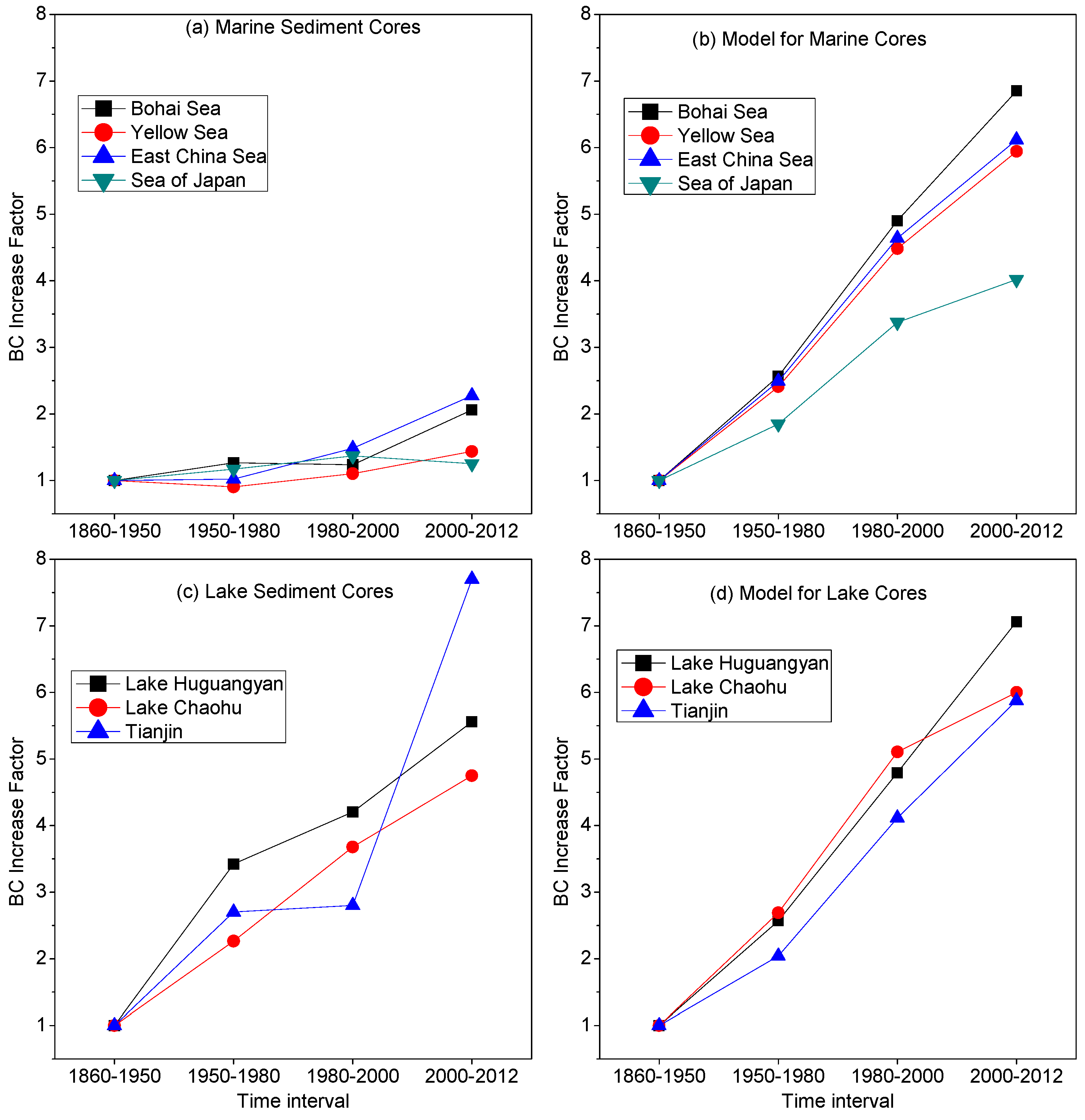
Figure 3.
Spatial variations in BC increase factor and its correlation to BC fluxes. (a) Correlation between increase factor and BC fluxes for marine sediment cores (g m−2 yr−1) and model simulations (mg m−2 yr−1). (b) Spatial variations in BC increase factor according to GISS simulation (shaded pattern) and sediment core measurements (circles) for the period of 2000–2012. (c) Spatial map of surface sediment BC fluxes [31] and (d) the derived BC increase factors.


Table 1.
Marine and lake sediment cores used in this work.
| Site | Longitude, Latitude | Sample Setting | Source |
|---|---|---|---|
| Marine sediment cores | |||
| SJP15 | 136.49° E, 44.10° N | Sea of Japan, water depth 885 m | This study |
| SJP17 | 134.69° E, 42.85° N | Sea of Japan, water depth 1164 m | This study |
| SJP19 | 133.96° E, 40.05° N | Sea of Japan, water depth 732 m | This study |
| NYS | 122.48° E, 38.16° N | Northern Yellow Sea, water depth 50 m | [13] |
| SYS | 123.50° E, 34.99° N | Southern Yellow Sea, water depth 76 m | [13] |
| Bohai Sea | 119.27° E, 38.60° N | Central mud area in the Bohai Sea, water depth 27 m | [13] |
| ECS1 | 122.50° E, 29.00° N | East China Sea, northern Min Zhe coastal mud area, water depth 50 m | [13] |
| ECS2 | 121.66° E, 27.64° N | East China Sea, southern Min Zhe coastal mud area, water depth 50 m | [13] |
| Sediment cores in China | |||
| Tianjin | 117.51° E, 38.77° N | Three parallel cores from a wetland/marsh in the south of Tianjin, north China | This study |
| Lake Chaohu | 117.50° E, 31.50° N | One of the famous “five freshwater lakes” in Anhui Province of eastern China. Average water depth is ~2.7 m | [37] |
| Lake Huguangyan | 110.28° E, 21.15° N | A maar lake with a natural sediment trap in southeastern China. Average water depth is ~20 m | [37] |
Table 2.
BC fluxes and increase factors in four time periods. BC fluxes are shown in average values along with standard deviation (S.D.). The time interval 1860–1950 is considered the pre-industrial period due to the almost flat trend of BC fluxes in most cores and all model simulations. The increase factor of BC fluxes for each period is the ratio of the considered time interval to the 1860–1950 levels.
| 1860–1950 | 1950–1980 | 1980–2000 | 2000–2012 | |||||
|---|---|---|---|---|---|---|---|---|
| Average | S.D. # | Average | S.D. # | Average | S.D. # | Average | S.D. # | |
| Fluxes (g m−2 yr−1) | ||||||||
| Bohai Sea | 4.7 | 0.6 | 6.0 | 1.0 | 5.8 | 1.5 | 9.7 | 2.1 |
| Yellow Sea | 1.4 | 0.3 | 1.3 | 0.2 | 1.5 | 0.6 | 2.0 | 0.4 |
| East China Sea | 9.2 | 2.8 | 9.4 | 2.4 | 13.6 | 5.2 | 20.8 | 4.9 |
| Sea of Japan | 1.4 | 0.4 | 1.7 | 0.9 | 2.0 | 0.8 | 1.8 | 0.6 |
| Tianjin | 0.6 | 0.4 | 1.6 | 1.3 | 1.6 | 0.9 | 4.5 | 2.2 |
| Lake Chaohu | 0.3 | 0.1 | 0.6 | 0.1 | 1.0 | 0.3 | 1.3 | 0.2 |
| Lake Huguangyan | 0.11 | 0.02 | 0.36 | 0.10 | 0.45 | 0.03 | 0.59 | 0.08 |
| Increase Factor | ||||||||
| Bohai Sea | 1.0 | 1.3 | 1.2 | 2.1 | ||||
| Yellow Sea | 1.0 | 0.9 | 1.1 | 1.4 | ||||
| East China Sea | 1.0 | 1.0 | 1.5 | 2.3 | ||||
| Sea of Japan | 1.0 | 1.2 | 1.4 | 1.3 | ||||
| Tianjin | 1.0 | 2.7 | 2.8 | 7.7 | ||||
| Lake Chaohu | 1.0 | 2.3 | 3.7 | 4.7 | ||||
| Lake Huguangyan | 1.0 | 3.4 | 4.2 | 5.6 |
# S.D. stands for standard deviation.
Table 3.
The percentage of missing BC in marine sediment for core profiles and surface.
| Site | 1950–1980 | 1980–2000 | 2000–2012 | Surface | Average | S.D. # |
|---|---|---|---|---|---|---|
| Bohai Sea | 50.6 | 74.8 | 69.9 | 74.0 | 67.3 | 11.3 |
| Yellow Sea | 62.4 | 75.4 | 75.8 | 73.3 | 71.7 | 6.3 |
| East China Sea | 58.9 | 68.0 | 62.8 | N.A. | 63.2 | 4.6 |
| Sea of Japan | 36.5 | 59.4 | 68.8 | N.A. | 54.9 | 16.6 |
| Total Average | 52.1 | 69.4 | 69.3 | 73.7 | 65.1 | 11.1 |
| Total S.D. | 11.5 | 7.4 | 5.3 | 0.5 | 7.1 | 5.4 |
# S.D. stands for standard deviation.
Disclaimer/Publisher’s Note: The statements, opinions and data contained in all publications are solely those of the individual author(s) and contributor(s) and not of MDPI and/or the editor(s). MDPI and/or the editor(s) disclaim responsibility for any injury to people or property resulting from any ideas, methods, instructions or products referred to in the content. |
© 2023 by the authors. Licensee MDPI, Basel, Switzerland. This article is an open access article distributed under the terms and conditions of the Creative Commons Attribution (CC BY) license (https://creativecommons.org/licenses/by/4.0/).
Share and Cite
MDPI and ACS Style
Chen, B.; Tiwari, S.; Liu, K.; Zou, J. More Than Half of Emitted Black Carbon Is Missing in Marine Sediments. Sustainability 2023, 15, 9739. https://doi.org/10.3390/su15129739
AMA Style
Chen B, Tiwari S, Liu K, Zou J. More Than Half of Emitted Black Carbon Is Missing in Marine Sediments. Sustainability. 2023; 15(12):9739. https://doi.org/10.3390/su15129739
Chicago/Turabian StyleChen, Bing, Shani Tiwari, Kun Liu, and Jianjun Zou. 2023. "More Than Half of Emitted Black Carbon Is Missing in Marine Sediments" Sustainability 15, no. 12: 9739. https://doi.org/10.3390/su15129739
Note that from the first issue of 2016, this journal uses article numbers instead of page numbers. See further details here.