
A Novel Sustainable Reverse Logistics Network Design for Electric Vehicle Batteries Considering Multi-Kind and Multi-Technology
1
Energy Economy Research Center, School of Business Administration, Henan Polytechnic University, Jiaozuo 454003, China
2
School of Finance and Economics Administration, Henan Polytechnic University, Jiaozuo 454003, China
*
Author to whom correspondence should be addressed.
Sustainability 2023, 15(13), 10128; https://doi.org/10.3390/su151310128
Submission received: 22 May 2023
/
Revised: 19 June 2023
/
Accepted: 24 June 2023
/
Published: 26 June 2023
(This article belongs to the Section Waste and Recycling)
Abstract
:With the expansion of the new energy vehicle market, electric vehicle batteries (EVBs) have entered a massive retirement wave. The strategic level of facility location and configuration decisions and the tactical level of multi-product flow and multi-technology selection decisions have been integrated into a sustainable reverse logistics network (SRLN). In this paper, we considered multiple kinds of waste electric vehicle batteries (WEVBs) with multiple recycling technology and constructed a multi-level SRLN model for WEVBs with the objectives of minimum economic costs and minimum carbon emissions. To solve this model, fuzzy set theory was applied to the equivalence transformation of constraints, non-interactive and interactive methods were used to solve the multi-objective planning (MOP), and interactive fuzzy programming with priority control was proposed to find the global optimal solution for this model. Finally, numerical experiments demonstrated the feasibility and effectiveness of the proposed model and solution method. The experimental results show that the SRLN model considering carbon emissions can significantly reduce carbon emissions of the network through a slight increase in the initial network construction cost, thus effectively balancing both economic and environmental objectives. In the non-interactive solution, the Lp-metric method has a lower deviation index than the weighted sum method; in the interactive solution, the priority control method proposed in this paper outperforms the TH method in terms of the number of practical solutions and CPU time and shows strong performance in searching and finding optimal solutions. The proposed model and method can provide the theoretical basis and technical support for a WEVB SRLN under the limited information uncertainty environment.
1. Introduction
With rising energy prices, nuclear energy issues and climate change, the need to rely on more renewable energy is growing [1], and new energy vehicles powered by EVBs as a vehicle choice have become the automotive industry’s future development direction. The UK plans to ban new diesel and gasoline car sales by 2030 [2]; China has become the world’s largest producer and consumer of electric vehicles for six consecutive years, with cumulative sales totaling more than 50,000 units [3]. As the average lifetime of EVBs is eight years [4], early battery products are gradually entering the retirement stage. The number of waste electric vehicle batteries (WEVBs) is expected to reach 1.68 million units by 2030, or about 848,000 tons [5].
It is significant to recycle WEVBs. If they are echelon-used and regenerated, this can alleviate the resource shortage. After decommissioning, a WEVB still has 80% of its capacity, still has enough performance for other scenarios [6], and can be used in communication base stations, low-speed electric vehicles, and other fields for echelon-use. Energy storage not only provides technical solutions for grid operators to ensure a balance between production and consumption but also enables the best use of renewable resources [7]. Richa et al. [8] investigated the environmental benefits of WEVB in stationary energy storage. The results showed that the cumulative net global warming potential was reduced by 15% through reuse. Moreover, this reduction can reach 70% under ideal refurbishment and reuse conditions. Therefore, reuse is undoubtedly a promising solution for managing WEVBs. Recycling the valuable materials of WEVBs can not only create substantial economic benefits but also slow down the demand for virgin resources and reduce the risk of relying on imports. If not handled properly, heavy metals, electrolytes, and plastic will cause severe environmental pollution and safety hazards [9]. WEVB recycling is a hot spot of global concern, which is both the end of the sustainable development of the new energy industry and the key to a green and sustainable supply of strategic resources such as nickel, cobalt, and lithium. Therefore, it is necessary to establish a complete and efficient WEVB recycling system to cope with the massive wave of decommissioning.
Li et al. [10] analyzed the current situation and prospects of WEVB recycling in China. Zou et al. [11] suggested developing WEVB recycling in two respects: further strengthening the construction of a policy and standard system, and increasing support for WEVB recycling enterprises. Some scholars also discussed WEVB recycling from the perspective of recycling mode and there are four recycling modes for retired WEVBs: battery manufacturer-led mode, automobile manufacturer-led mode, manufacturer alliance-led mode, and third-party-led mode [12]. In this paper, we took automobile manufacturers as the main recycling body and built an SRLN. WEVBs can be divided into ternary lithium batteries and lithium iron phosphate batteries according to the cathode material [13], as shown in Table 1. Waste ternary lithium batteries have a high metal content, a short life cycle, and their safety is greatly reduced after the battery capacity decays; their treatment mainly takes the form of disassembly and recycling to achieve the recycling of nickel, cobalt, manganese, lithium, and other resources. In contrast, wasted lithium iron phosphate batteries still have better recyclability and safety, so they will first be echelon-used and then regenerated [14]. Before 2016, the new EVBs in China were mainly lithium iron phosphate batteries [15], so lithium iron phosphate batteries will be the first to enter the peak of retirement.
In the sustainable development model, regardless of whether WEVB is refurbished or not, the material will eventually need to be recycled and landfill or incineration disposal needs to be minimized. Currently, the main focus is on recovering valuable and rare metals from cathode materials. Physical pretreatment is usually used first to improve the material recovery rate. The aim is to obtain different waste streams to ensure adequate separation of the different components within the material for further processing. Subsequently, hydrometallurgical or pyrometallurgical technologies are used to extract metals or other impurities from specific waste streams and then further process the recovered material [16]. Extractive metallurgy (including pyrometallurgy and hydrometallurgy) is the most common technology used in the industry to recover valuable rare metals from cathode materials and provides an economical alternative to mining raw high-value elements such as cobalt and nickel [17]. Umicore is a large international recycling company that uses both pyrometallurgy and hydrometallurgy technologies but mainly pyrometallurgy-dominant technology [18]. Most recycling companies in China (e.g., GEM and Brunp) use hydrometallurgical technology [19]. Sumitomo Sony in Japan uses pyrometallurgical technology [20]. However, the disadvantages of pyrometallurgy are low recovery rates and high carbon emissions, while the disadvantages of hydrometallurgy are long recovery processes and high chemical consumption [21], with significant differences in economic and environmental impacts, as shown in Table 2. Pyrometallurgical technology refers to the recovery of refined valuable metals from waste lithium-ion battery materials using physical or chemical transformation at high temperatures and, finally, the resulting alloys and slags are treated separately and further purified from the metal monomers. Hydrometallurgy technology is a method for recovering valuable metals by dissolving the valuable metal oxides in the cathode active material into metal ions by leaching, and then the leachate is treated with precipitation, ion exchange, solvent extraction, and electrolysis to remove impurities or separate metals [22].
With the introduction of carbon-neutral policies, countries are paying more and more attention to environmental protection. Since WEVBs have a significant impact on the environment, their reverse logistics process has been a critical issue, where a good RLN becomes a prerequisite for waste recycling, cost reduction, profit increase, and efficiency improvement. With the in-depth practice of the sustainable development concept and the increasingly significant environmental and social impacts of reverse logistics activities, the sustainable reverse logistics network design (SRLND) issue is becoming a hot research topic. Drawing on the definition of the concept of logistics network design in the literature [23], the SRLND focused on in this paper refers to the planned layout of the entire distribution channel from the place of consumption to the point of recycling or proper disposal of recycled resources or waste, oriented to at least two of the economic, environmental, and social objectives. Facility siting plays a crucial and central role in RLND, which is usually costly to build, cannot be easily modified, and increases CO2 emissions. Therefore, this paper considered cost and CO2 emissions in reverse logistics network design to ensure the economic and environmental performance of the SRLN.
In this paper, we addressed the following two objectives: to construct an optimization model for a generic RSLN for WEVBs that minimizes economic costs and environmental impacts under a complete fuzzy environment by considering multiple recycling options, multiple regeneration technologies, and multiple kinds of batteries in order to solve this problem using various effective and well-performing solution methods to find economic and environmental compromise solutions to achieve global optimality.
At present, research on the design and optimization of RLN for WEVB recycling is relatively limited and still in the exploratory stage, and some relevant literature has relatively simple research perspectives, such as not considering the impact of multiple regeneration treatment technologies and multiple kinds of batteries on the economic and environmental benefits of reverse logistics networks, which is somewhat different from the complex reality. The research in this paper will further enrich the existing work in this field and the novelty and contributions of this work are summarized as follows:
(1) This paper proposed a multi-objective combinatorial optimization model for the recycling of WEVB. The MOP model was developed with the objectives of minimum economic costs and minimum carbon emissions in a fuzzy environment. It is more reasonable and better reflects the concept of sustainable development than simply considering economic or environmental objectives;
(2) We considered a multiple recycling strategy: remanufacturing, reuse, and regeneration. We considered two kinds of WEVBs in the SRLN—ternary lithium batteries and lithium iron phosphate batteries—as well as two technologies in the regeneration treatment stage—pyrometallurgy and hydrometallurgy—so that the constructed SRLN has universality;
(3) An interactive fuzzy method with priority control was used to improve the solving capability and to obtain a solution that satisfies the decision maker (DM) through continuous interaction. The validity and feasibility of the model and method were verified using extensive simulation results, and some management and policy insights were given;
The rest of this paper is organized as follows. Section 2 overviews the most relevant literature and outlines the main contributions. Section 3 describes the RLND problem studied in this paper and constructs an MOP model in an uncertain environment. The solution method of the fuzzy multi-objective planning (FMOP) model is presented in Section 4. Numerical experiments were designed and are analyzed in Section 5 and, finally, conclusions are presented in Section 6.
2. Literature Review
2.1. RLND
Since the 1990s, with the increasing pressure on environmental resources, the strengthening of government regulations, the shortening of product life cycles, the enhancement of consumer awareness of environmental protection, and the intensification of business competition, reverse logistics activities have gradually received social attention. Unlike forward logistics, reverse logistics involves the reuse, recycling, remanufacturing, waste disposal, and other operational activities of various waste products, as well as the accompanying collection, storage, transportation, and other logistics activities [24], which have the characteristics of high complexity, multi-linkedness, and uncertainty. These characteristics make the operation of a reverse logistics system more dependent on logistics network support. RLND is a strategic decision that profoundly impacts the whole system’s operation and is generally regarded as the primary and most crucial task in reverse logistics management [25].
Uncertainty is one of the essential characteristics of reverse logistics, which is becoming a factor to be considered in more and more mathematical models for RLND. Existing studies mainly consider the uncertainty of demand, cost and price factors, and technical parameters for used and waste products. Most of them only consider the uncertainty of a single parameter. Karagoz et al. [26] evaluated the uncertainty of the number of end-of-life vehicles and proposed a scenario-based real-life stochastic optimization model to improve end-of-life vehicles in Istanbul’s supply chain network management. However, there are two main drawbacks to using stochastic methods: (1) in many real-life scenarios, there are not enough historical data for the uncertain parameters, so we can rarely obtain actual and accurate stochastic distributions of the uncertain parameters. In addition, the chance constraint significantly increases the computational complexity of the original problem; (2) in previous work on inverse supply chain network design under uncertainty, most uncertainty has been modeled by scenario-based stochastic programming. The many scenarios representing uncertainty can make the computation challenging in these cases. As an alternative, fuzzy set theory [27] provided a framework to deal with different types of uncertainty, including fuzzy coefficients for lack of knowledge or cognitive uncertainty and flexibility of constraints and objectives. Shukla et al. [28] considered the dynamic, flexible capacity of different facilities to study the dynamic flexibility on the performance of RLN with the objectives of maximizing profit and minimizing carbon emissions; Golpîra et al. [29] considered demand uncertainty and constructed a risk-based closed-loop supply chain network model from economic and social dimensions.
Different recycled products have other characteristics. In the field of WEVB recycling, due to the different losses of batteries, their recycling quality is also different, and they need to be tested and classified for their quality level. At present, most of the WEVBs in China go to small black market workshops with low operating costs, high recycling prices, and unregulated operations, so the recycling quantity is uncertain. Since the WEVB recycling network is yet to be improved and will face a sharp increase in WEVBs in the next few years, new facilities at all levels may need to be built or re-planned, so it becomes necessary to carry out research that includes more uncertainties, such as battery recycling price, cost per unit of battery disposal, carbon emissions at all levels and facilities, and transportation distance and cost.
2.2. RLND for WEVBs
A large amount of literature has been published on WEVB recycling issues, such as WEVB recycling strategies [30,31], recycling technologies [32,33], and recycling modes [34,35]. The research on WEVBs regeneration technology and recycling mode decisions has been relatively mature. However, there are relatively few studies on RLND and this research is still in the exploration stage.
The literature on RLND for WEVBs can be divided into single-objective and multi-objective models. Li et al. [36] established a mixed-integer nonlinear programming model with the objective of profit maximization. Kamyabi et al. [37] established a two-stage mixed-integer stochastic programming model with the aim of profit maximization and conducted SD simulations. Wang et al. [38] explored the impact of the carbon tax on the design of WEVB recycling networks with the objective of costs minimization. Masudin et al. [39] developed an RLN model for battery recycling considering environmental costs and manufacturing costs. Hu et al. [40] constructed an RLN considering carbon emission costs to construct profit maximization as the objective. Compared with the RLND considering only a single objective (usually to minimize costs or maximize profit), multi-objective optimization is more reasonable and practical in practical applications. Subsequently, scholars have expanded the objectives from economic costs to other aspects, forming a multi-objective model for a more comprehensive network design. Yang et al. [41] constructed a mixed integer programming model to minimize costs, minimize waste emissions, and maximize job opportunities. Guan et al. [42] established a WEVB recycling network under the third-party recycling model with the objectives of minimizing costs and minimizing adverse social effects. Liu et al. [43] constructed a mixed integer programming model with the objectives of maximizing profit and minimizing carbon emissions. Alkahtani et al. [44] constructed a battery RLN that minimizes economic costs and environmental impact and maximizes employment opportunities. Subula et al. [45] constructed a closed-loop supply chain network that minimizes costs and maximizes recycling scope. Mu et al. [46] constructed a sustainable six-level dynamic RLN model that minimizes costs, and environmental and social impacts. Table 3 lists the published literature on the design of reverse networks for WEVBs.
2.3. MOP Solution Method
MOP has been widely used in different fields for many years. In real life, several uncertainties often need to be considered when solving MOP. Therefore, FMOP has been widely studied. Based on the DM’s preference for the objectives, the existing methods for solving MOP in various real-life settings can be divided into non-interactive and interactive methods [47].
Non-interactive methods have a priori and a posteriori decision-making methods. The priori decision-making methods provide preference information to the DM before solving the optimization problem, transforming the multi-objective problem into a single-objective problem. This method has been widely used due to its relatively low computational complexity. However, obtaining accurate preference information in practical situations is difficult because the DM needs more knowledge of the optimization problem to solve it without background knowledge. The a posteriori decision is made after the optimization problem is solved. The desired solution from the entire set of solutions approximates the objective space according to the preference requirements. This method is computationally high-cost and time-consuming, and it is challenging to handle high-dimensional multi-objective optimization problems.
To address the weaknesses of non-interactive methods, interactive methods have been improved and developed accordingly. Compared with non-interactive methods, such as the Lp-metric and weighted sum methods, interactive methods can involve DMs in the model solving process and achieve more satisfactory optimal solutions for DMs. This is very important because the RLND of WEVBs is still in the early stage of design and will face a dramatic increase in the recycling volume in the next few years, so the deep involvement of DMs is needed. In this paper, we adopted an interactive decision method that can flexibly measure and adjust the satisfaction level of each objective function interactively and progressively according to the DM’s preferences, and the DM can gradually give the preferences in each iteration, adjust and correct the preference information in time, and dynamically guide the search process of the algorithm, which can better ensure that the optimal solution that meets the DM’s target preference requirements is finally obtained. This method can provide more accurate preference information than the a priori method, and the DM has a smaller selection burden, which can overcome the shortcomings of the a priori and a posteriori methods. In interactive method research, Zimmermann [48] developed a fuzzy method for solving MOP called the maximum-minimum method. Later, Lai and Hwang [49] refined the maximum-minimum method approach; Li et al. [50] proposed a two-stage fuzzy method; Selim and Ozkarahan [51], and Torabi and Hassini [52] effectively compensated for the original shortcomings by adding the coefficient of compensation to the model.
However, their use has some limitations: some may not yield effective solutions or only give a few solutions. Some methods require a two-stage solution or specify a target level, which may be difficult for DM. Therefore, this paper proposes a priority-controlled interactive fuzzy planning approach to compensate for the weaknesses of these methods [53]. Instead of specifying target values for each objective, the model is controlled by weight coefficient and compensation coefficients, using the last priority objective and the constraint of compensation coefficients. With this improvement, the model can produce more effective solutions than existing methods, which is a strength of the method. In addition, the best solution can be easily selected by adjusting the minimum satisfaction level of the last priority objective and compensation coefficient, which is more flexible than the existing methods.
3. Problem Description and Proposed Model
In this paper, the research system boundary covered the process from recovery to recycling WEVBs to reduce costs and carbon emissions. As shown in Figure 1, the network can be divided into five main parts: recycling, disassembling, testing, remanufacturing, recombination, and regeneration, and it consists of recycling markets, battery replacement points, testing centers, remanufacturing centers, energy storage centers, and disposal centers. First, WEVBs are collected from the recycling market through the replacement point and transported to the testing center. The testing center disassembles the WEVBs into battery modules, considers the health status of the WEVBs, and conducts quality-level testing and classification, which mainly include testing parameters such as battery capacity, internal resistance, and self-discharge. Battery State of Health (SOH) reflects the overall performance of the battery and its ability to store electrical energy. Among them, SOH is most commonly defined by the degree of battery capacity decay [54]:
Caged is the battery’s current capacity and Crated is the battery’s rated capacity. It is known that the larger the SOH value of the battery, the better the performance of the battery.
Combined with relevant information, this paper divided WEVBs into two recycling states: echelon-use and regeneration. It treated them differently and applied them to different scenarios to realize the organic combination of resource recycling and high-value utilization:
Level 1(L1)—Echelon-use, for WEVBs with SOH at 100–20%, shipped to the echelon-use enterprises. Among them, batteries with SOH greater than 80% are sent to the remanufacturing centers, where they can be repaired and capacitated to improve their performance and applied to the electric vehicle service scenario [38]; batteries with SOH of 80–20% are shipped to the energy storage center and mainly applied to the energy internet storage scenario through restructurings, such as communication base stations or low-speed electric vehicles with slightly lower power requirements.
Level 2(L2)—Regeneration, for WEVBs with SOH decaying to less than 20%, shipped to the disposal center. Through recycling technologies such as pyrometallurgy or hydrometallurgy, WEVBs completely disposed of are crushed, dismantled, and smelted to extract valuable metals and materials, which are later applied to produce new batteries.
3.1. Assumptions
The main assumptions considered in the presented model are as follows:
- (1)
- The recycling market, as the source region of WEVB recycling, is known and fixed in location;
- (2)
- The transportation cost of WEVBs is linearly related to the transportation distance and quantity;
- (3)
- The transportation process of WEVBs does not have cross-level transportation, and all follow the planned path in the RLN;
- (4)
- The alternative locations and quantities of replacement points, testing centers, remanufacturing centers, energy storage centers, and disposal centers are known and have a maximum processing capacity limit.
3.2. Notations
Set the set, parameters, and variables of the model according to the set modeling context.
3.2.1. Indices
| E | Set of WEVB product kinds, e∈ {1, 2, ..., E}; |
| I | Set of recycling markets, i∈{1, 2, ..., I}; |
| J | Set of replacement points, j∈{1, 2, ..., J}; |
| K | Set of testing centers, k∈{1, 2, ..., K}; |
| L | Set of remanufacturing centers, l∈{1, 2, ..., L}; |
| M | Set of energy storage centers, m∈{1, 2, ..., M}; |
| N | Set of disposal centers, n∈{1, 2, ..., N}; |
| T | Set of technologies used by the disposal centers, t∈{1, 2, ..., T}; |
3.2.2. Parameters
| Fj | Fixed construction cost of replacement point; |
| Fk | Fixed construction cost of the testing center; |
| Fl | Fixed construction cost of remanufacturing center; |
| Fm | Fixed construction cost of the energy storage center; |
| Fnt | Fixed construction cost of disposal center with t-technology; |
| Oje | Operating cost per unit e-kind of WEVBs at the replacement point; |
| Oke | Operating cost per unit e-kind of WEVBs at the testing center; |
| Ole | Operating cost per unit e-kind of WEVBs at the remanufacturing center; |
| Ome | Operating cost per unit e-kind of WEVBs at the energy storage center; |
| Onte | Operating cost per unit e-kind of WEVBs at disposal center with t-technology; |
| Hj | Maximum processing capacity of the replacement point; |
| Hk | Maximum processing capacity of the testing center; |
| Hl | Maximum processing capacity of the remanufacturing center; |
| Hm | Maximum processing capacity of the energy storage center; |
| Hnt | Maximum processing capacity of disposal center with t-technology; |
| Rj | Carbon emission from building a replacement point; |
| Rk | Carbon emission from building a testing center; |
| Rl | Carbon emission from building a remanufacturing center; |
| Rm | Carbon emission from building an energy storage center; |
| Rnt | Carbon emission from building a disposal center with t-technology; |
| Sje | Carbon emission from processing units e-kind of WEVBs at replacement point; |
| Ske | Carbon emission from processing unit e-kind of WEVBs in testing center; |
| Sle | Carbon emission from processing unit e-kind of WEVBs in remanufacturing center; |
| Sme | Carbon emission from processing unit e-kind of WEVBs in energy storage center; |
| Snte | Carbon emission from processing unit e-kind of WEVBs in disposal centers with t-technology; |
| Dij | Distance between recycling market and replacement point; |
| Djk | Distance between the replacement point and the testing center; |
| Dkl | Distance between the testing center and remanufacturing center; |
| Dkm | Distance between the testing center and energy storage center; |
| Dkn | Distance between the testing center and disposal center; |
| W | Carbon emission per unit transport distance for a unit battery; |
| Qie | Number of WEVBs of e-kind of WEVBs recovered by recycling market i; |
| Pe | Recycling price per unit e-kind of WEVBs at the replacement point; |
| U | Transportation cost per unit distance of unit battery; |
| be | Proportion of e-kind of WEVBs used for echelon-use; |
| ce | Proportion of the number of e-kind of WEVBs shipped to remanufacturing centers to the number of e-kind of WEVBs for echelon-use; |
3.2.3. Variables
| Xj | Binary variable equal to 1 if replacement point j is opened, and 0 otherwise; |
| Xk | Binary variable equal to 1 if testing center k is opened, and 0 otherwise; |
| Xl | Binary variable equal to 1 if remanufacturing center l is opened, and 0 otherwise; |
| Xm | Binary variable equal to 1 if energy storage center m is opened, and 0 otherwise; |
| Xnt | Binary variable equal to 1 if disposal center n uses t-technology, and 0 otherwise; |
| Qije | Integer variable indicating the number of e-kind of WEVBs shipped from recycling market i to battery replacement point j; |
| Qjke | Integer variable indicating the number of e-kind of WEVBs shipped from replacement point j to testing center k; |
| Qkle | Integer variable indicating the number of e-kind of WEVBs shipped from testing center k to remanufacturing center l; |
| Qkme | Integer variable indicating the number of e-kind of WEVBs shipped from testing center k to energy storage center m; |
| Qke | Integer variable indicating the number of e-kind of WEVBs that can be echelon-used from testing center k; |
| Qknte | Integer variable indicating the number of e-kind of WEVBs from testing center k to disposal center n with t-technology. |
3.3. Model Construction
Based on the problem description and the above model assumptions and notation, this paper established a multi-objective mixed integer linear programming model M1 under an uncertain environment to minimize the logistics network’s total costs and carbon emissions.
3.3.1. Objective Functions
The economic cost objective function (ECOF) consists of the construction costs of fixed facilities (FC), transportation costs (TC), operation costs of facilities (OC), and recycling price costs (PC). Among them, FC is the sum of the construction costs of fixed facilities of the replacement point, testing center, remanufacturing center, energy storage center, and disposal center; TC is the sum of transportation costs between each level in the RLN; OC is the sum of operation and processing costs of the replacement point, testing center, remanufacturing center, energy storage center, and disposal center; PC is the recycling costs of WEVBs at the replacement point.
The low carbon objective function (LCOF) consists of fixed facility construction carbon emissions (BCE), transportation carbon emissions (TCE), and facility operation carbon emissions (OCE). Among them, BCE is the sum of fixed construction carbon emissions of replacement points, testing centers, remanufacturing centers, energy storage centers, and disposal centers; TCE is the sum of transportation carbon emissions between each level in the RLN; OCE is the sum of operational treatment carbon emissions of replacement points, testing centers, remanufacturing centers, energy storage centers, and disposal centers.
3.3.2. Constraints
s.t.
Constraint (11) guarantees that WEVBs in the recycling market must be recycled; Constraint (12) indicates the flow balance before and after the WEVB replacement point; Constraint (13) indicates the flow balance constraint before and after the testing center; Constraint (14) defines the number of WEVBs received from the testing center by the laddering enterprise; Constraint (15) represents the relationship between the number of batteries that can be echelon-used by the testing center and the amount of recycling; Constraint (16) represents the relationship between the number of remanufacturing and the number of batteries that can be echelon-used; Constraint (17) means that each disposal center can only choose at most one process to dispose of WEVBs; Constraints (18)–(22) represent the maximum processing capacity constraints of the replacement point, testing center, remanufacturing center, energy storage center, and disposal center, respectively; Constraints (23) and (24) define the range of variable-taking values.
4. Proposed Solution Methodology
The proposed model is an FMOP model. Firstly, the original model waws converted into an equivalent auxiliary crisp model to solve this model. Secondly, the multi-objective model was transformed into a single-objective model using both non-interactive and interactive methods.
4.1. The Equivalent Auxiliary Crisp Model
Assume that is a triangular fuzzy number and ; the following equation can be defined as the membership:
According to [55], the expected interval (EI) and expected value (EV) of fuzzy triangular numbers can be defined as follows:
According to the ranking method for any pair of fuzzy numbers and , the degree in which is bigger than is defined as follows:
Additionally, according to the definition of fuzzy equations [56], for any pair of fuzzy numbers and it will be said that is indifferent (equal) to in degree of if the following relationships hold simultaneously:
The above equations can be rewritten as follows:
Now, we consider the following fuzzy mathematical programming model in which all parameters are defined as triangular fuzzy numbers:
According to [57], it is feasible in degree . Equations (28) and (29) and are equivalent to the following ones, respectively:
These equations can be rewritten as follows:
Similarly, by using the ranking method, it can be proved that a feasible solution like x0 is an -acceptable optimal solution of the model (31) if and only if for all feasible decision vectors say x such that , and , the following equation holds:
Therefore, x0 is a better choice (with the objective of minimizing) at least in degree 1/2 as opposed to the other feasible vectors. The above equation can be rewritten as follows:
Consequently, using the definition of expected interval and expected value of a fuzzy number, the equivalent crisp -parametric model of the model (31) can be written as follows:
According to the above descriptions, the equivalent auxiliary crisp model of the M1 model can be formulated as M2:
4.2. Multi-Objective Planning Solution Method
Increasingly, research focuses on multi-objective optimization and balancing rather than on considering only a single objective.
4.2.1. Lp-Metric Method
This method minimizes the distance of the objective function in a multi-objective model [58]. In other words, it tries to minimize the distance of the objective function value from the ideal point, as shown in Equation (57):
Here, wj denotes the weights of the jth objective function value and p denotes the degree of emphasis on the deviation (1 < p < ∞). In this study, the value of p was taken as 1. Weights are given so that the sum of the wj is 1. The value shows the optimum value that the jth objective function value can take when considered individually.
4.2.2. Weighted Sum Method
In the weighted sum method, a weight wj is assigned to each objective function j and the weighted sum of objectives is minimized, as shown in Equation (58):
This approach obtains the non-dominated solution by trying different weights wj. The weighted sum method has been extended using a linear membership function with normalization [59]. In this case, the objective function is normalized and takes values between 0 and 1. The main goal of the weighted sum method is to maximize the satisfaction of both objectives by obtaining the best classification result. The goal is to maximize the total satisfaction value of both objectives simultaneously. denote the value of the function that maximizes and minimizes objective 1, denote the value of the function that maximizes and minimizes objective 2. The satisfaction of objective 1 is , and the satisfaction of objective 2 is , as shown in Equation (59):
4.2.3. Improved Fuzzy Interactive Solution Method
This paper used an interactive fuzzy planning method with priority control. The proposed model is a single-phase interactive fuzzy programming approach that has a max-min term and a compensatory term with a priority constraint. The detailed steps of the fuzzy interaction solution method are as follows:
Step 1: Given the confidence level , solve the positive ideal solution () and the negative ideal solution () for the two objectives of model M2, respectively.
(1) In the TH method, the maximum and minimum values of single-objective optimization are solved separately and used to represent the respective ideal solutions as shown in Equation (60), which requires four calculations.
(2) This paper solved the minimum values of carbon emissions and costs in single-objective optimization separately to represent the respective positive and negative ideal solutions. The positive and negative ideal solutions of each objective are shown in Equation (61). Equation (61) is the optimal solution for the minimum cost value and the optimal solution for the minimum carbon emission value.
Compared with the TH method, the method in this paper can reduce the carbon emission objective search space [], the cost objective search space [], and the computational effort, thus improving the solution efficiency.
Step 2: Determine a linear membership function for each objective function as follows:
where denotes the satisfaction degree of hth objective function.
Step 3: Transform the multi-objective model M2 into the following single-objective model M3, as follows:
(1) TH aggregation function:
where F(x) is the domain of feasible solutions constituted by the constraints of the clear equivalence model; denotes the minimum satisfaction degree of objectives, respectively. This formulation has a new achievement function defined as a convex combination of the lower bound for satisfaction degree of objectives (), and the weighted sum of these achievement degrees () to ensure yielding an adjustably balanced compromise solution. Moreover, and γ indicate the relative importance of the hth objective function and the coefficient of compensation, respectively. The parameters are determined by the DM based on her/his preferences such that . Additionally, γ controls the minimum satisfaction level of objectives as well as the compromise degree among the objectives implicitly.
(2) Improved aggregation function:
The first priority objective and the last priority objective are determined. The adjustment term of the TH fuzzy method is modified by defining the weight of the first priority objective as equal to 1, and the coefficient of the weight of the other objectives is 0. The coefficient of compensation is set only for the first priority objective, eliminating the weight constraint in the TH fuzzy method.
where F(x) is the domain of feasible solutions constituted by the constraints of M2; denotes the minimum satisfaction level of all objective functions, and is the minimum satisfaction level of the first priority objective; γ is the coefficient of compensation of all objectives; is the minimum satisfaction level of the last priority objective.
Step 4: Define the coefficient of compensation (γ) and the minimum satisfaction () and solve the proposed model. To find the balanced solution, define 0.5 and the coefficient of compensation γ is 0.99. Then, obtain the value of the membership function of the last priority objective as the upper bound of the . If the equilibrium solution is satisfactory, then stop. Otherwise, proceed to Step 5.
Step 5: Interactively update the coefficient of compensation and the minimum satisfaction. If the coefficient of compensation is zero, then the model would not have a minimum satisfaction level for all objective functions and would solve only the first priority objective function. The solution would not compensate for each objective and an efficient solution would not be guaranteed. Moreover, if the coefficient of compensation is equal to one, it is a max-min model. So, γ should be greater than zero and less than one. The value of the membership function of the last priority objective obtained in Step 4 is used as the upper bound of the . Therefore, the value of is adjusted between (0~] and the value of γ is adjusted in the range of (0,0.99] and, then, the valid solution is found. If the DM is satisfied with the obtained solution, the current solution is the optimal solution and the current solution is also the optimal solution, then the calculation stops; otherwise, the values of γ and are changed to define other valid solutions according to the DM’s preferences for economic and environmental objectives, values are increased or decreased according to the confidence level expected by the DM, and Step 5 or Step 1 is turned.
In summary, the method for solving the fuzzy multi-objective model in this paper is shown in Figure 2:
5. Numerical Experiments
5.1. Data Generation
As shown in Figure 3, there are six recycling markets, five replacement point candidates, four testing center candidates, two remanufacturing center candidates, three energy storage center candidates, and three disposal center candidates in the RLN of WEVBs in Tianjin. Two kinds of WEVBs are recycled, and two technologies are used in the disposal centers.
To generate the triangular fuzzy parameters, based on Lai and Hwang [49], the three prominent points (i.e., the most likely, the most pessimistic, and the most optimistic values) are estimated for each imprecise parameter. To do so, each parameter’s most likely () value is first generated randomly (using the uniform distributions specified in Table 4). When the proposed crisp model is used, the corresponding crisp value is assumed to equal the most likely value for all parameters. After that, without loss of generality two random numbers (r1, r2) are generated between 0.2 and 0.8 using uniform distribution, and the most pessimistic () and optimistic () values of a fuzzy number () are calculated as follows:
For large operating truck transportation (load: 4–8 tons), the fuel consumption is about 19.04~25.37 L/100 km; therefore, according to the carbon emission density of diesel fuel 0.848 kg/L, the emission factor of CO2 can be obtained as about 0.514 kg/km [60]. According to the China Road Freight Transport Price Index released by the Ministry of Transport, it is known that the average transportation cost of an ordinary truck is about 0.33 yuan/ton/km, since ordinary trucks are considered to transport WEVBs. According to the average battery recycling price, waste lithium iron phosphate batteries are about 4000 yuan/ton and waste ternary batteries are about 8900 yuan/ton. The confidence level was set to 0.9 and other parameters were set as shown in Table 4.
5.2. Analysis of the Solution Process
This paper solved this problem on a computer with AMD (R) Core (TM) R5-5625U CPU @ 2.30 GHz RAM 16.00 GB 64-bit, Windows 11. The mathematical model was solved with the Lingo 18.0 software. The positive ideal solution () and negative ideal solution () for the two objectives of the problem were calculated as follows:
Therefore, the linear membership functions of the two objectives are:
The interactive fuzzy planning with priority control is shown in Equation (69):
Taking carbon emission as the first priority objective, when the minimum satisfaction level is 0.5 and the coefficient of compensation γ is 0.9, is 0.575. Its value is used as the upper bound of the . The results of the coefficient of compensation and minimum satisfaction of the interactive adjustment are shown in Table 5 and Table 6.
Table 5 shows that the γ value affects the balanced and unbalanced solutions and, if a balanced solution is needed, a high value of the coefficient of compensation should be assigned. When the value of γ is 0.8~0.9 and they are close to each other, indicating that the two objectives of economic and environmental are relatively balanced. The interaction can be stopped if the DM is satisfied and the optimal solution is output. Table 6 shows the minimum satisfaction level of the economic objective, and the value of affects the direction of the solution. If the value of is small, it means that the influence of the economic objective on the solution is small and the solution is directed to the environmental objective solution; if the value of is large, it indicates the influence of the economic objective on the solution is large.
5.3. Experiment Analysis
5.3.1. Analysis of Results
Set the coefficient of compensation γ = 0.9 and the minimum satisfaction = 0.5 when the DM can obtain a relatively balanced solution. The objective cost value is 28,520,770 yuan, and the carbon emissions are 108,202 kg. Figure 4 shows the location of logistics facilities at various levels and the number of different kinds of WEVBs handled. Figure 5 and Figure 6 show the costs and carbon emissions ratio of the total process accounted for by each link in the WEVB recycling process.
5.3.2. Parametric Impact Analysis
Since the recycling quantity and the ratio of echelon-use are uncertain, which largely affects the layout of the logistics network and facility construction, the range of their values is now deflated, and the perturbation changes of the optimal solution of the model are obtained within the specified step. As the massive retirement of WEVBs under the warranty period and the lifetime constraint will lead to a significant increase in the future recycling volume, the value of recycling quantity is changed in the range of [0, +20%] with a step of 5%; since the echelon-use technology largely determines the sustainable development level of WEVB recycling industry, the value of the echelon-use ratio is changed in the range of [−10%, +10%] with a step of 5%. The results are shown in Figure 6.
The results show that, with the increment of recycling quantity, the number of WEVBs in the RLN increases and the costs and carbon emissions increase accordingly; with the increment of the ratio of echelon-use, the number of WEVBs shipped to echelon-use enterprises increases, and the costs and carbon emissions decrease subsequently because the costs and carbon emissions of echelon-use are smaller than those of regeneration.
5.4. Model Comparison
The RLND model with a single cost or carbon emission objective was introduced and compared with the optimization results of the multi-objective model constructed in this paper.
As can be seen from Table 7, the single-objective model can achieve the optimal value on a single objective compared to the multi-objective model. Still, on the other hand, the aspect performs worse. If only the cost single objective is considered, its cost is the smallest, but the carbon emissions are larger, and the disposal centers all choose the lower cost of pyrometallurgy. On the contrary, when the DM wants to optimize the carbon emission objective, the solution will determine the technology and facilities with more minor carbon emissions, and the costs will increase at this time. In this paper, the RLN model considering carbon emissions can significantly reduce the carbon emissions of the network by increasing the initial network construction cost by a small amount, effectively considering both economic and environmental objectives.
5.5. Comparative Analysis of Methods
5.5.1. Comparison of Non-Interactive Methods
The deviation index indicates the rational state of each solution concerning the respective ideal and lowest points [61]. Thus, the deviation index is a criterion that indicates the suitability of a particular decision technique for a given optimization problem. The smaller the value it obtains, the more appropriate the technique is. Therefore, it is necessary to calculate the deviation of the results obtained by different decision methods concerning the ideal and minimum points, as shown in Equation (70):
where denotes the value of the objective function fj at the ideal and non-ideal points.
5.5.2. Comparison of Interactive Methods
- Comparison of effective solution numbers
Table 10 compares the results of interactive fuzzy planning with priority control and TH methods. At γ values from 0.1 to 0.9, the interactive fuzzy planning with a priority-controlled method can calculate multiple solutions based on the satisfaction of the last priority objective. The TH fuzzy method solves this by adjusting the coefficient of the weight of each objective by adding 0.1. The interactive fuzzy planning with priority control can produce eight valid solutions, more than TH fuzzy methods, as shown in Figure 7.
- Comparison of CPU time
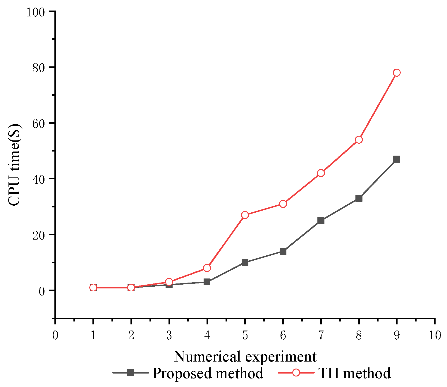
The proposed model was tested on nine different numerical experiment scales. The computation time of the proposed model is shown in Table 11. The CPU times of all the numerical experiments solved using the method of this paper, the TH method, are shown in Figure 8. It can be seen from Figure 8 that the CPU time of both methods changes slightly as the problem size increases. In addition, the results show that the method proposed in this paper outperforms the TH method in this research model and can solve large-scale problems in a reasonable and faster time.
6. Conclusions
In this paper, we studied the design of an SRLN for WEVBs from the perspective of sustainable development, with two objectives minimizing costs and carbon emissions. A generic and practical network structure was proposed to support multiple recycling options, such as remanufacturing, reuse, and regeneration, in a configuration consistent with the relationship between environmental protection and economic development. In addition, considering two kinds of WEVB in RLN and two technologies in the regeneration treatment stage shows practical implications in reality. Two non-interactive and two interactive methods were applied to solve the MOP problem, and interactive fuzzy programming with priority control was proposed to find a compromise solution that satisfies both objective functions simultaneously to find the global optimal value for the model. In addition, numerical experiments compared the proposed MOP methods in detail, and the results illustrate the feasibility of the proposed models and solutions.
From the perspective of management decisions, this paper provided theoretical guidance and a decision basis for the layout of the reverse logistics network of WEVBs. It provided strategic and tactical references for achieving sustainable development while improving the economic efficiency of enterprises. From the analysis, it can be concluded that the level of echelon-use of WEVBs greatly influences the reduction of logistics network costs and carbon emissions. Usually, the echelon-use relies heavily on rapid sorting technology, and a large amount of traceability information is required in this process. However, most of this information is stored by upstream companies, such as battery production information from battery manufacturers and battery operation information from electric vehicle manufacturers. Considering the different interests of all companies, it is still very difficult to share this information adequately. Therefore, development of the recycling of WEVBs requires continuous policy guidance and pilot work.
Future work will focus on the design of closed-loop logistics networks for WEVB considering front-end forward logistics and, for large stochastic mixed-integer planning, some advanced solution methods, i.e., metaheuristic algorithms, should be developed to improve computational efficiency and effectiveness.
Author Contributions
Conceptualization, Z.F. and Y.L.; methodology, Z.F.; software, Y.L; validation, Z.F., Y.L. and S.L.; formal analysis, Y.L.; investigation, N.L.; resources, S.L.; data curation, N.L.; writing—original draft preparation, Y.L.; writing—review and editing, N.L.; visualization, Z.F.; supervision, Y.L.; project administration, S.L.; funding acquisition, Z.F. All authors have read and agreed to the published version of the manuscript.
Funding
This work was partly supported by the grants from the National Natural Science Foundation of China (Grant No. 71502050), the Philosophy and Social Science Planning Project of Henan Province, China (Grant No. 2022BJJ048) and Henan Polytechnic University’s Young Backbone Faculty Grant Program (Grant No. 2019XQG-21).
Institutional Review Board Statement
Not applicable.
Informed Consent Statement
Not applicable.
Data Availability Statement
Not applicable.
Acknowledgments
The authors especially thank the Editors and anonymous referees for their kind review and helpful comments.
Conflicts of Interest
The authors declare no conflict of interest.
References
- Soliman, M.S.; Belkhier, Y.; Ullah, N.; Achour, A.; Alharbi, Y.M.; Al Alahmadi, A.A.; Abeida, H.; Khraisat, Y.S.H. Supervisory energy management of a hybrid battery/PV/tidal/wind sources integrated in DC-microgrid energy storage system. Energy Rep. 2021, 7, 7728–7740. [Google Scholar] [CrossRef]
- Sithole, H.; Cockerill, T.T.; Hughes, K.J.; Ingham, D.B. Developing an optimal electricity generation mix for the UK 2050 future. Energy 2016, 100, 363–373. [Google Scholar] [CrossRef] [Green Version]
- Zeng, B.; Li, H.; Mao, C.; Wu, Y. Modeling, prediction and analysis of new energy vehicle sales in China using a variable-structure grey model. Expert Syst. Appl. 2023, 213, 118879. [Google Scholar] [CrossRef]
- Tang, Y.; Zhang, Q.; Li, Y.; Wang, G. Recycling mechanisms and policy suggestions for spent electric vehicles’ power battery—A case of Beijing. J. Clean. Prod. 2018, 186, 388–406. [Google Scholar] [CrossRef]
- Yao, P.F.; Huang, Q.; Zhang, X.H.; Li, H. Recycling potentials of critical resources from spent lithium-ion power batteries in China. Chin. J. Rare Met. 2022, 46, 1331–1339. [Google Scholar]
- Winslow, K.M.; Laux, S.J.; Townsend, T.G. A review on the growing concern and potential management strategies of waste lithium-ion batteries. Resour. Conserv. Recycl. 2018, 129, 263–277. [Google Scholar] [CrossRef]
- Al Alahmadi, A.A.; Belkhier, Y.; Ullah, N.; Abeida, H.; Soliman, M.S.; Khraisat, Y.S.H.; Alharbi, Y.M. Hybrid wind/PV/battery energy management-based intelligent non-integer control for smart DC-microgrid of smart university. IEEE Access 2021, 9, 98948–98961. [Google Scholar] [CrossRef]
- Richa, K.; Babbitt, C.W.; Nenadic, N.G.; Gaustad, G. Environmental trade-offs across cascading lithium-ion battery life cycles. Int. J. Life Cycle Assess. 2017, 22, 66–81. [Google Scholar] [CrossRef]
- Lander, L.; Cleaver, T.; Rajaeifar, M.A.; Nguyen-Tien, V. Financial viability of electric vehicle lithium-ion battery recycling. Iscience 2021, 24, 102787. [Google Scholar] [CrossRef]
- Li, Y.; Liu, Y.; Chen, Y.; Huang, S.; Ju, Y. Estimation of end-of-life electric vehicle generation and analysis of the status and prospects of power battery recycling in China. Waste Manag. Res. 2022, 40, 1424–1432. [Google Scholar] [CrossRef]
- Zou, R.R.; Liu, Q. Current situation and Countermeasures of power battery recycling industry in China. Conf. Ser. Earth Environ. Sci. 2021, 702, 012013. [Google Scholar] [CrossRef]
- Zhou, X.; Li, J.; Li, F.; Deng, X. Recycling supply chain model of new energy vehicle power battery based on Blockchain technology. Comput. Integr. Manuf. Syst. 2023, 29, 1386. [Google Scholar]
- Wang, F.F.; Feng, X.M.; Zhao, G.J.; Xia, D.W. Identification of retired power lithium-ion batteries of chemical systems by electrochemical impedance spectroscopy. Energy Storage Sci. Technol. 2023, 12, 609–614. [Google Scholar]
- Liu, Z.; Liu, X.; Hao, H.; Zhao, F. Research on the Critical Issues for Power Battery Reusing of New Energy Vehicles in China. Energies 2020, 13, 1932. [Google Scholar] [CrossRef] [Green Version]
- Deng, X.T. Analysis of the entire industry chain of power battery recycling. Resour. Recycl. 2023, 48, 40–48. [Google Scholar]
- Lv, W.; Wang, Z.; Cao, H.; Sun, Y.; Zhang, Y.; Sun, Z.H. A critical review and analysis on the recycling of spent lithium-ion batteries. ACS Sustain. Chem. Eng. 2018, 6, 1504–1521. [Google Scholar] [CrossRef]
- Steward, D.; Mayyas, A.; Mann, M. Economics and challenges of Li-Ion battery recycling from end-of-life vehicles. Procedia Manuf. 2019, 33, 272–279. [Google Scholar] [CrossRef]
- Assefi, M.; Maroufi, S.; Yamauchi, Y.; Sahajwalla, V. Pyrometallurgical recycling of Li-ion, Ni–Cd and Ni–MH batteries: A minireview, current opinion in green and sustainable. Chemistry 2020, 24, 26–31. [Google Scholar]
- Liu, C.; Lin, J.; Cao, H.; Zhang, Y.; Sun, Z. Recycling of spent lithium-ion batteries in view of lithium recovery: A critical review. J. Clean. Prod. 2019, 228, 801–813. [Google Scholar] [CrossRef]
- Fujita, T.; Chen, H.; Wang, K.-T.; He, C.-L.; Wang, Y.-B.; Dodbiba, G.; Wei, Y.-Z. Reduction, reuse and recycle of spent Li-ion batteries for automobiles: A review. Int. J. Miner. Metall. Mater. 2021, 28, 179–192. [Google Scholar] [CrossRef]
- Energy, N. Recycle spent batteries. Nat. Energy 2019, 4, 253. [Google Scholar]
- Chen, W.; Liang, J.; Yang, Z.; Li, G. A review of lithium-ion battery for electric vehicle applications and beyond. Energy Procedia 2019, 158, 4363–4368. [Google Scholar] [CrossRef]
- Eskandarpour, M.; Dejax, P.; Miemczyk, J.; Péton, O. Sustainable supply chain network design: An optimization-oriented review. Omega 2015, 54, 11–32. [Google Scholar] [CrossRef]
- Zhang, X.; Zou, B.; Feng, Z.; Wang, Y. A review on remanufacturing reverse logistics network design and model optimization. Processes 2022, 10, 84. [Google Scholar] [CrossRef]
- Lambert, S.; Riopel, D.; Abdul-Kader, W. A reverse logistics decisions conceptual framework. Comput. Ind. Eng. 2011, 61, 561–581. [Google Scholar] [CrossRef]
- Karagoz, S.; Aydin, N.; Simic, V. A novel stochastic optimization model for reverse logistics network design of end-of-life vehicles: A case study of Istanbul. Environ. Model. Assess. 2022, 27, 599–619. [Google Scholar] [CrossRef]
- Zadeh, L.A. Fuzzy sets as a basis for a theory of possibility. Fuzzy Sets Syst. 1978, 1, 3–28. [Google Scholar] [CrossRef]
- Shukla, M.; Vipin, B.; Sengupta, R.N. Impact of dynamic flexible capacity on reverse logistics network design with environmental concerns. Ann. Oper. Res. 2022, 1–26. [Google Scholar] [CrossRef]
- Golpîra, H.; Javanmardan, A. Robust optimization of sustainable closed-loop supply chain considering carbon emission schemes. Sustain. Prod. Consum. 2022, 30, 640–656. [Google Scholar] [CrossRef]
- Zhang, C.; Chen, Y.X. Decision and coordination of cascade utilization power battery closed-loop supply chain with economies of scale under government subsidies. Oper. Res. Manag. 2021, 30, 72–77+91. [Google Scholar]
- Zhao, X.; Peng, B.; Zheng, C.; Wan, A. Closed-loop supply chain pricing strategy for electric vehicle batteries recycling in China. Environ. Dev. Sustain. 2022, 24, 7725–7752. [Google Scholar] [CrossRef]
- Pappu, S.; Muduli, S.; Katchala, N.; Tata, N.R. Easy and scalable synthesis of NiMnCo-Oxalate electrode material for supercapacitors from spent Li-Ion batteries: Power source for electrochromic devices. Energy Fuels 2022, 36, 13398–13407. [Google Scholar] [CrossRef]
- Zhou, J.; Bing, J.; Ni, J.; Wang, X. Recycling the waste LiMn2O4 of spent Li-ion batteries by pH gradient in neutral water electrolyser. Mater. Today Sustain. 2022, 20, 100205. [Google Scholar] [CrossRef]
- Zhang, C.; Chen, Y.X.; Tian, Y.X. Collection and recycling decisions for electric vehicle end-of-life power batteries in the context of carbon emissions reduction. Comput. Ind. Eng. 2023, 175, 108869. [Google Scholar] [CrossRef]
- Xie, J.Y.; Le, W.; Guo, B.H. Pareto Equilibrium of New Energy Vehicle Power Battery Recycling Based on Extended Producer Responsibility. Chin. J. Manag. Sci. 2022, 30, 309–320. [Google Scholar]
- Li, L.; Dababneh, F.; Zhao, J. Cost-effective supply chain for electric vehicle battery remanufacturing. Procedia Eng. 2018, 226, 277–286. [Google Scholar] [CrossRef]
- Kamyabi, E.; Moazzez, H.; Kashan, A.H. A hybrid system dynamics and two-stage mixed integer stochastic programming approach for closed-loop battery supply chain optimization. Appl. Math. Model. 2022, 106, 770–798. [Google Scholar] [CrossRef]
- Wang, L.; Wang, X.; Yang, W. Optimal design of electric vehicle battery recycling network–From the perspective of electric vehicle manufacturers. Appl. Energy 2020, 275, 115328. [Google Scholar] [CrossRef]
- Masudin, I.; Saputro, T.E.; Arasy, G.; Jie, F. Reverse logistics modeling considering environmental and manufacturing costs: A case study of battery recycling in Indonesia. Int. J. Technol. 2019, 10, 189–199. [Google Scholar] [CrossRef] [Green Version]
- Yang, Y.X.; Guan, Q. Sustainable reverse logistics network optimization model based on dual-channel power battery recycling mode. Comput. Integr. Manuf. Syst. 2022. accepted. [Google Scholar]
- Guan, Q.; Yang, Y. Reverse logistics network design model for used power battery under the third-party recovery mode. In Proceedings of the 2020 16th International Conference on Computational Intelligence and Security (CIS), Nanning, China, 1 November 2020. [Google Scholar]
- Liu, J.J.; Guo, Y.K. Design of reverse logistics network for electric vehicle power battery considering uncertainty. J. Shanghai Marit. Univ. 2021, 42, 96–102. [Google Scholar]
- Alkahtani, M.; Ziout, A. Design of a sustainable reverse supply chain in a remanufacturing environment: A case study of proton-exchange membrane fuel cell battery in Riyadh. Adv. Mech. Eng. 2019, 11, 1–14. [Google Scholar]
- Subulan, K.; Baykasoğlu, A.; Özsoydan, F.B.; Taşan, A.S. A case-oriented approach to a lead/acid battery closed-loop supply chain network design under risk and uncertainty. J. Manuf. Syst. 2015, 37, 340–361. [Google Scholar] [CrossRef]
- Liao, G.H.W.; Luo, X. Collaborative reverse logistics network for electric vehicle batteries management from the sustainable perspective. J. Environ. Manag. 2022, 324, 116352. [Google Scholar] [CrossRef]
- Mu, N.; Wang, Y.; Chen, Z.S.; Xin, P. Multi-objective combinatorial optimization analysis of the recycling of retired new energy electric vehicle power batteries in a sustainable dynamic reverse logistics network. Environ. Sci. Pollut. Res. 2023, 30, 47580–47601. [Google Scholar] [CrossRef]
- Rosenthal, R.E. Concepts, theory, and techniques principles of multi-objective optimization. Decis. Sci. 1985, 16, 133–152. [Google Scholar]
- Zimmermann, H.J. Fuzzy programming and linear programming with several objective functions. Fuzzy Sets Syst. 1978, 1, 45–55. [Google Scholar] [CrossRef]
- Lai, Y.J.; Hwang, C.L. Possibilistic linear programming for managing interest rate risk. Fuzzy Sets Syst. 1993, 54, 135–146. [Google Scholar] [CrossRef]
- Selim, H.; Ozkarahan, I. A supply chain distribution network design model: An interactive fuzzy goal programming-based solution approach. Int. J. Adv. Manuf. Technol. 2008, 36, 401–418. [Google Scholar] [CrossRef]
- Li, X.Q.; Zhang, B.; Li, H. Computing efficient solutions to fuzzy multiple objective linear programming problems. Fuzzy Sets Syst. 2006, 157, 1328–1332. [Google Scholar] [CrossRef]
- Torabi, S.A.; Hassini, E. An interactive possibilistic programming approach for multiple objective supply chain master planning. Fuzzy Sets Syst. 2008, 159, 193–214. [Google Scholar]
- Jarernsuk, S.; Phruksaphanrat, B. A new interactive fuzzy programming with priority control for multi-objective decision-making problems. J. Intell. Fuzzy Syst. 2022, 43, 7779–7792. [Google Scholar] [CrossRef]
- Wang, C.; Yuan, Z.Y.; Wang, Y.W.; Cao, W.J. Overview of key technologies for echelon utilization of decommissioned power batteries. Adv. New Renew. Energy 2021, 9, 327–341. [Google Scholar]
- Jiménez, M. Ranking fuzzy numbers through the comparison of its expected intervals. Int. J. Uncertain. Fuzziness Knowl.-Based Syst. 1996, 4, 379–388. [Google Scholar] [CrossRef]
- Parra, M.A.; Terol, A.B.; Gladish, B.P.; Urıa, M.R. Solving a multi-objective possibilistic problem through compromise programming. Eur. J. Oper. Res. 2005, 164, 748–759. [Google Scholar] [CrossRef]
- Jiménez, M.; Arenas, M.; Bilbao, A.; Rodrı, M.V. Linear programming with fuzzy parameters: An interactive method resolution. Eur. J. Oper. Res. 2007, 177, 1599–1609. [Google Scholar] [CrossRef]
- Abdolazimi, O.; Esfandarani, M.S.; Shishebori, D. Design of a supply chain network for determining the optimal number of items at the inventory groups based on ABC analysis: A comparison of exact and meta-heuristic methods. Neural Comput. Appl. 2021, 33, 6641–6656. [Google Scholar] [CrossRef]
- Chakraborty, D.; Guha, D.; Dutta, B. Multi-objective optimization problem under fuzzy rule constraints using particle swarm optimization. Soft Comput. 2016, 20, 2245–2259. [Google Scholar] [CrossRef]
- Peng, M.C.; Li, J.R.; Hu, H.F. Research on fuel consumption & carbon emission factor of road freight trucks. Automob. Technol. 2015, 475, 37–40. [Google Scholar]
- Ahmadi, M.H.; Sayyaadi, H.; Dehghani, S.; Hosseinzade, H. Designing a solar powered Stirling heat engine based on multiple criteria: Maximized thermal efficiency and power. Energy Convers. Manag. 2013, 75, 282–291. [Google Scholar] [CrossRef]
Figure 1.
WEVBs recycling mechanism map.
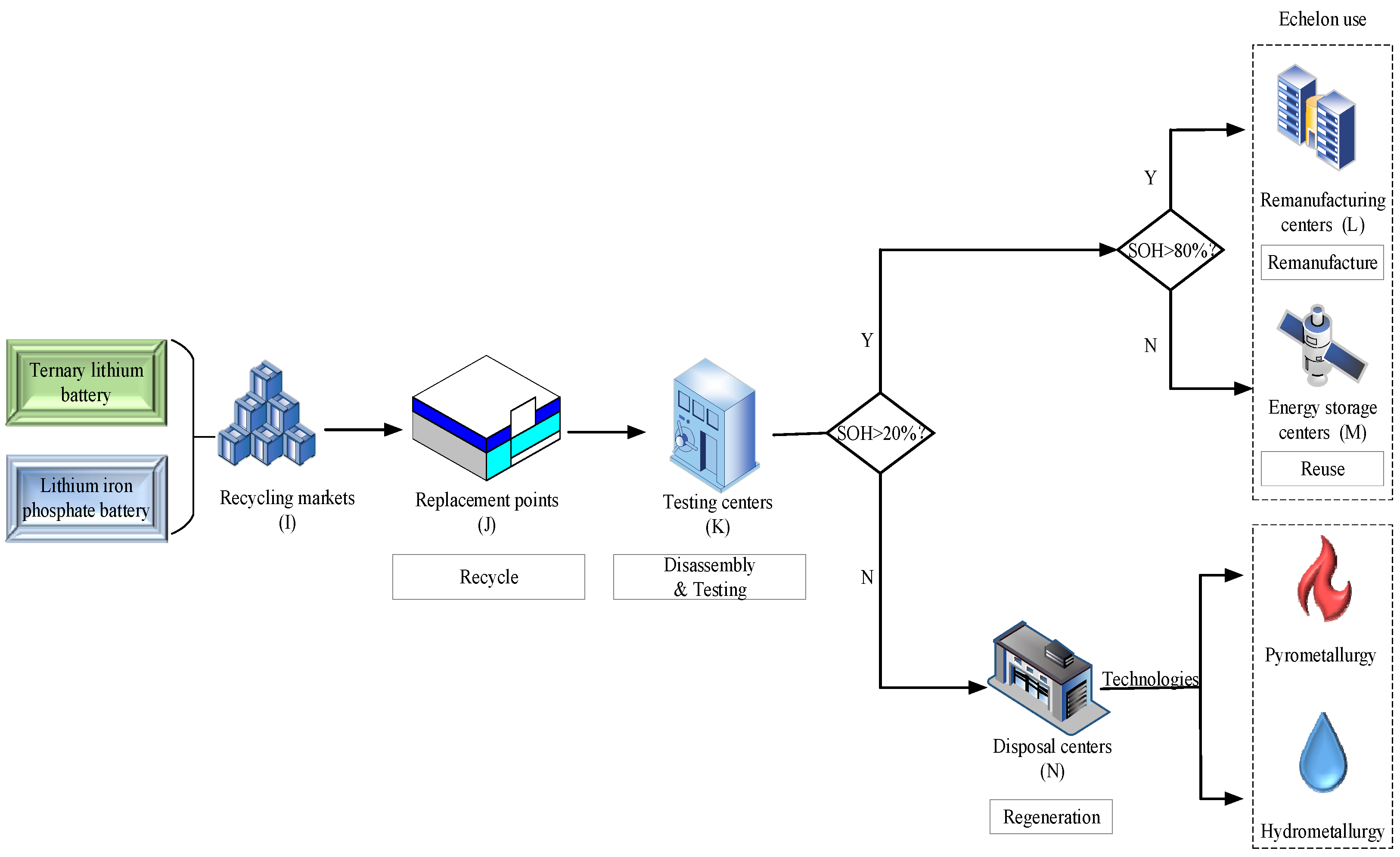
Figure 2.
The flowchart of the proposed method.
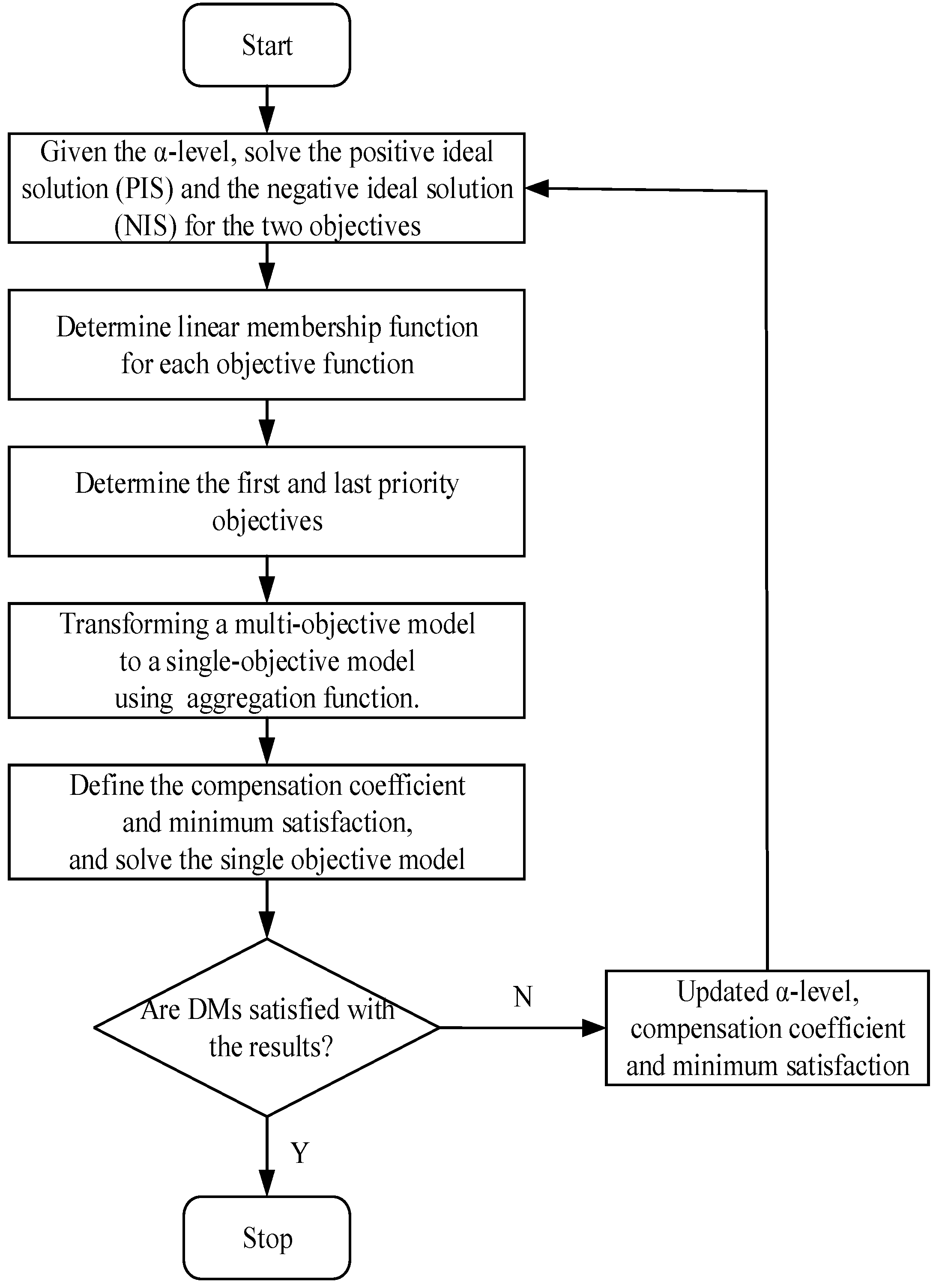
Figure 3.
Proposed construction of logistics facilities.
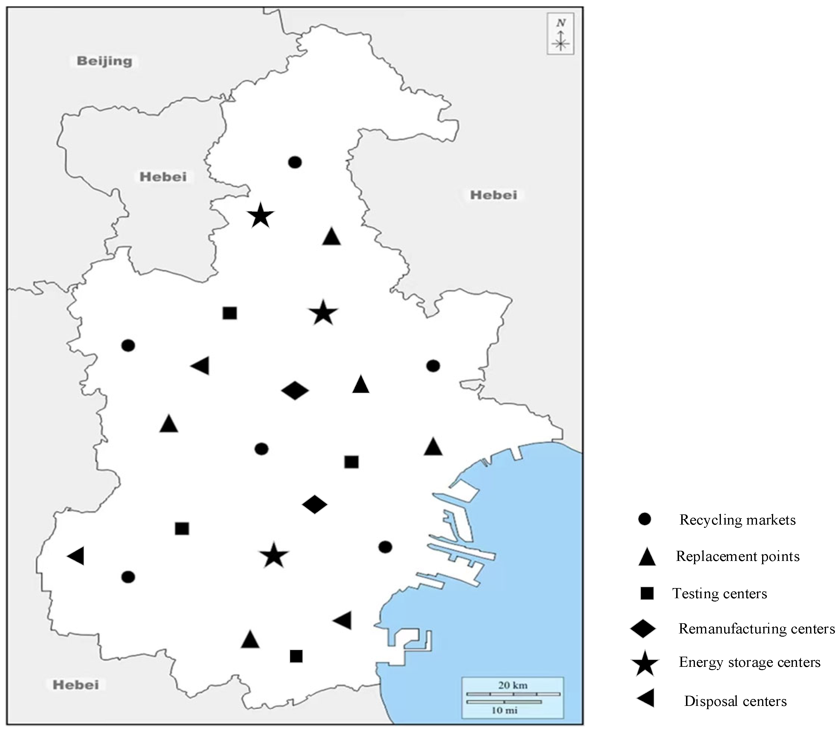
Figure 4.
Siting of logistics facilities at all levels and the number of different kinds of WEVBs handled.
Figure 4.
Siting of logistics facilities at all levels and the number of different kinds of WEVBs handled.

Figure 5.
(a) The proportion of the costs of each link; (b) The proportion of carbon emissions of each link.
Figure 5.
(a) The proportion of the costs of each link; (b) The proportion of carbon emissions of each link.

Figure 6.
(a) The objective function value under the change of the number of recycling; (b) The objective function value under the change of the echelon-use ratio.
Figure 6.
(a) The objective function value under the change of the number of recycling; (b) The objective function value under the change of the echelon-use ratio.
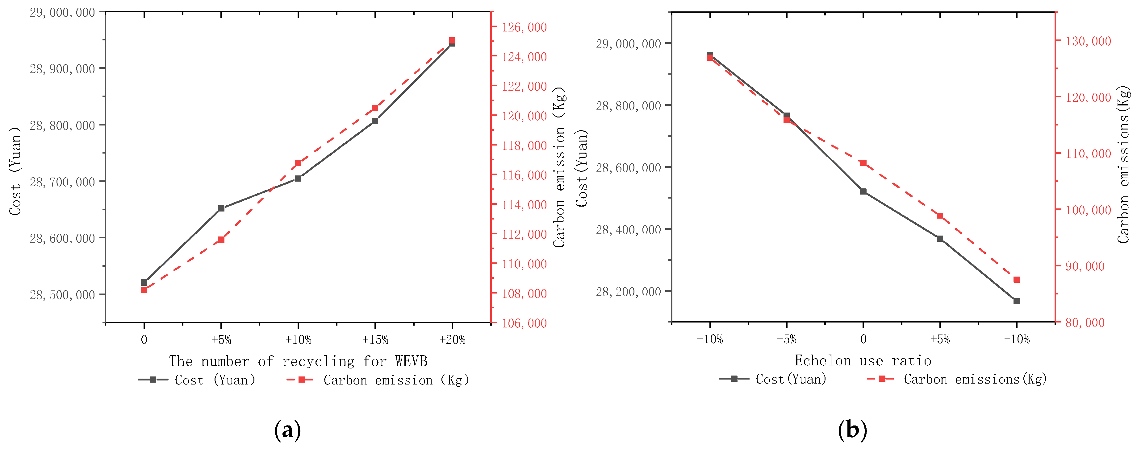
Figure 7.
(a) Solution results of the proposed method; (b) Solution results of TH method.

Figure 8.
Comparison of CPU time between the proposed and TH method under different numerical experiment scales.
Figure 8.
Comparison of CPU time between the proposed and TH method under different numerical experiment scales.

Table 1.
Ternary lithium battery and lithium iron phosphate battery comparison.
| WEVB Kinds | Cycle Life | Capacity Decay | Security | Cost |
|---|---|---|---|---|
| Ternary lithium battery | 3500 times | Faster | Poor | Higher (with precious metals) |
| Lithium iron phosphate battery | 2000 times | Slower | High | Lower (no precious metals) |
Table 2.
WEVB recycling technologies’ characteristics.
| Technologies | Advantages | Disadvantages |
|---|---|---|
| Pyrometallurgy | Simple process, low economic costs | High environmental impact, high carbon emissions |
| Hydrometallurgy | Low environmental impact, low carbon emissions | Complex process, high economic costs |
Table 3.
A summary of reviewed papers published for WEVBs.
| Authors | Carbon Emission | Model Type | WEVB Kind | Technology | Single Objective | Multi-Objective | ||||
|---|---|---|---|---|---|---|---|---|---|---|
| Certainty | Uncertainty | Single | Dual | Single | Dual | Non- Interactive | Interactive | |||
| Li [36] | √ | √ | √ | √ | ||||||
| Kamyabi [37] | √ | √ | √ | √ | ||||||
| Wang [38] | √ | √ | √ | √ | ||||||
| Masudin [39] | √ | √ | √ | √ | ||||||
| Hu [40] | √ | √ | √ | √ | √ | |||||
| Yang [41] | √ | √ | √ | √ | √ | |||||
| Guan [42] | √ | √ | √ | √ | ||||||
| Liu [43] | √ | √ | √ | √ | √ | |||||
| Alkahtani [44] | √ | √ | √ | √ | ||||||
| Subulan [45] | √ | √ | √ | √ | ||||||
| Mu [46] | √ | √ | √ | √ | ||||||
| Our work | √ | √ | √ | √ | √ | |||||
Table 4.
Parameters range.
| Parameters | Corresponding Random Distribution |
|---|---|
| (Ұ) | U (1,500,000–3,700,000) |
| (Ұ) | U (500–2500) |
| (ton) | U (25–60) |
| (kg) | U (5000–8500) |
| (kg) | U (10–120) |
| (km) | U (5–50) |
| (ton) | U (15–20) |
| (ton) | U (10–15) |
| be1 | U (0.67–0.73) |
| be2 | U (0.27–0.43) |
| ce1 | U (0.45–0.5) |
| ce2 | U (0.15–0.25) |
Table 5.
Two objective satisfaction and function values when .
| 0.1 | 11.52 | 95.73 | 29,833,500 | 105,867 |
| 0.2 | 11.52 | 95.73 | 29,833,500 | 105,867 |
| 0.3 | 11.52 | 95.73 | 29,833,500 | 105,867 |
| 0.4 | 49.46 | 70.89 | 28,733,400 | 107,527 |
| 0.5 | 53.29 | 67.55 | 28,632,380 | 107,725 |
| 0.6 | 53.29 | 67.55 | 28,632,380 | 107,725 |
| 0.7 | 57.53 | 59.47 | 28,525,810 | 108,185 |
| 0.8 | 57.64 | 57.64 | 28,520,770 | 108,202 |
| 0.9 | 57.64 | 57.64 | 28,520,770 | 108,202 |
Table 6.
Two objective satisfaction and function values when .
| 0.1 | 11.52 | 95.73 | 29,833,500 | 105,867 |
| 0.2 | 34.04 | 73.57 | 29,139,460 | 107,369 |
| 0.3 | 41.72 | 72.59 | 28,937,090 | 107,427 |
| 0.4 | 53.29 | 67.55 | 28,632,380 | 107,725 |
| 0.5 | 57.18 | 60.11 | 28,529,930 | 108,165 |
| 0.575 | 57.64 | 57.64 | 28,520,770 | 108,202 |
Table 7.
Comparison of optimization results with the single-objective model.
| Model | Disposal Center | Technology | ||
|---|---|---|---|---|
| Proposed model | 28,520,770 | 108,202 | N(1) | Hydrometallurgy |
| N(2) | Pyrometallurgy | |||
| Cost single objective model | 27,402,270 | 111,719 | N(1) | Pyrometallurgy |
| N(2) | Pyrometallurgy | |||
| Carbon emission single objective model | 30,035,870 | 105,806 | N(1) | Hydrometallurgy |
| N(3) | Hydrometallurgy |
Table 8.
Deviation index of weighted sum method with different coefficients of weight.
| Weight | Value of the Objective Function | Deviation Index (Weighted Sum Method) | |||
|---|---|---|---|---|---|
| W1 | W2 | ||||
| 1 | 0 | 27,402,270 | 111,719 | 0.002 | |
| 0.9 | 0.1 | 27,414,470 | 111,020 | 0.005 | |
| 0.8 | 0.2 | 27,414,560 | 111,018 | 0.005 | |
| 0.7 | 0.3 | 27,414,560 | 111,018 | 0.005 | |
| 0.6 | 0.4 | 27,628,550 | 110,101 | 0.086 | |
| 0.5 | 0.5 | 28,632,380 | 107,725 | 0.467 | |
| 0.4 | 0.6 | 29,833,500 | 105,867 | 0.923 | |
| 0.3 | 0.7 | 29,833,500 | 105,867 | 0.923 | |
| 0.2 | 0.8 | 29,833,500 | 105,867 | 0.923 | |
| 0.1 | 0.9 | 30,035,870 | 105,806 | 0.998 | |
| 0 | 1 | 30,035,870 | 105,806 | 0.998 | |
| Average | 28,679,912 | 108,346 | 0.485 | ||
Table 9.
Deviation index of Lp-metric method with different coefficients of weight.
| Weight | Value of the Objective Function | Deviation Index (Lp-Metric Method) | |||
|---|---|---|---|---|---|
| W1 | W2 | ||||
| 1 | 0 | 27,402,270 | 111,719 | 0.002 | |
| 0.9 | 0.1 | 27,412,790 | 111,074 | 0.004 | |
| 0.8 | 0.2 | 27,414,470 | 111,020 | 0.005 | |
| 0.7 | 0.3 | 27,414,560 | 111,018 | 0.005 | |
| 0.6 | 0.4 | 27,414,560 | 111,018 | 0.005 | |
| 0.5 | 0.5 | 27,628,550 | 110,101 | 0.086 | |
| 0.4 | 0.6 | 27,628,550 | 110,101 | 0.086 | |
| 0.3 | 0.7 | 28,733,400 | 107,527 | 0.505 | |
| 0.2 | 0.8 | 29,833,500 | 105,867 | 0.923 | |
| 0.1 | 0.9 | 29,833,500 | 105,867 | 0.923 | |
| 0 | 1 | 30,035,870 | 105,806 | 0.998 | |
| Average | 28,250,184 | 109,192 | 0.322 | ||
Table 10.
The valid solutions of the proposed method and the TH method.
| Proposed Method | TH Method | |||
|---|---|---|---|---|
| 1 | 29,833,500 | 105,867 | 29,833,500 | 105,867 |
| 2 | 29,139,460 | 107,369 | 28,937,090 | 107,427 |
| 3 | 28,937,090 | 107,427 | 28,733,400 | 107,527 |
| 4 | 28,733,400 | 107,527 | 28,520,770 | 108,202 |
| 5 | 28,632,380 | 107,725 | ||
| 6 | 28,529,930 | 108,165 | ||
| 7 | 28,525,810 | 108,185 | ||
| 8 | 28,520,770 | 108,202 | ||
Table 11.
Numerical experiment scale.
| Scale | Numerical Experiments | Recycling Markets | Replacement Points | Testing Centers | Remanufacturing Centers | Energy Storage Centers | Disposal Centers |
|---|---|---|---|---|---|---|---|
| Small | 1 | 6 | 5 | 4 | 2 | 3 | 3 |
| 2 | 8 | 7 | 6 | 4 | 5 | 6 | |
| 3 | 10 | 9 | 8 | 6 | 7 | 7 | |
| Medium | 4 | 12 | 11 | 10 | 8 | 9 | 10 |
| 5 | 15 | 14 | 12 | 10 | 11 | 12 | |
| 6 | 17 | 16 | 14 | 12 | 13 | 14 | |
| Large | 7 | 20 | 18 | 16 | 14 | 15 | 15 |
| 8 | 25 | 23 | 21 | 19 | 20 | 21 | |
| 9 | 30 | 28 | 26 | 24 | 25 | 24 |
Disclaimer/Publisher’s Note: The statements, opinions and data contained in all publications are solely those of the individual author(s) and contributor(s) and not of MDPI and/or the editor(s). MDPI and/or the editor(s) disclaim responsibility for any injury to people or property resulting from any ideas, methods, instructions or products referred to in the content. |
© 2023 by the authors. Licensee MDPI, Basel, Switzerland. This article is an open access article distributed under the terms and conditions of the Creative Commons Attribution (CC BY) license (https://creativecommons.org/licenses/by/4.0/).
Share and Cite
MDPI and ACS Style
Fan, Z.; Luo, Y.; Liang, N.; Li, S. A Novel Sustainable Reverse Logistics Network Design for Electric Vehicle Batteries Considering Multi-Kind and Multi-Technology. Sustainability 2023, 15, 10128. https://doi.org/10.3390/su151310128
AMA Style
Fan Z, Luo Y, Liang N, Li S. A Novel Sustainable Reverse Logistics Network Design for Electric Vehicle Batteries Considering Multi-Kind and Multi-Technology. Sustainability. 2023; 15(13):10128. https://doi.org/10.3390/su151310128
Chicago/Turabian StyleFan, Zhiqiang, Yifan Luo, Ningning Liang, and Shanshan Li. 2023. "A Novel Sustainable Reverse Logistics Network Design for Electric Vehicle Batteries Considering Multi-Kind and Multi-Technology" Sustainability 15, no. 13: 10128. https://doi.org/10.3390/su151310128
Note that from the first issue of 2016, this journal uses article numbers instead of page numbers. See further details here.