
Energy and Fuel Consumption of a New Concept of Hydro-Mechanical Tractor Transmission
1
College of Mechanical and Electronic Engineering, Shandong Agricultural University, Taian 271018, China
2
Shandong Provincial Engineering Laboratory of Agricultural Equipment Intelligence, Taian 271018, China
3
College of Engineering, Nanjing Agricultural University, Nanjing 210031, China
4
College of Engineering, China Agricultural University, Beijing 100083, China
*
Author to whom correspondence should be addressed.
†
These authors contributed equally to this work.
Sustainability 2023, 15(14), 10809; https://doi.org/10.3390/su151410809
Submission received: 30 May 2023
/
Revised: 5 July 2023
/
Accepted: 7 July 2023
/
Published: 10 July 2023
(This article belongs to the Special Issue Mechanization and Intelligent Agricultural Devices towards the Future of Sustainability)
Abstract
:Tractors equipped with hydro-mechanical transmissions (HMTs) typically deliver excellent fuel-saving performance but are expensive. To improve the fuel economy of cheaper tractors, the authors of this study have designed an HMT for a tractor that uses a simple, single planetary gear to merge the power and analyze its consumption of energy and fuel. First, we introduce the principle of transmission of the HMT and formulate a model to calculate its speed, torque, and efficiency. Second, we analyze the parasitic power of the HMT and simulate its characteristics of efficiency. Finally, we compare the efficiency of transmission and fuel consumption of HMTs with a single planetary gear and Simpson planetary gears. The results showed that parasitic power was obtained when the displacement of the variable pump was negative and the maximum ratio of hydrostatic power in each range was 45–46%. The highest efficiency of the proposed HMT in ranges RL (low range) and RH (high range) were 87% and 89%, respectively. It has a simpler structure than the HMT with Simpson planetary gears and consumes lower amounts of energy and fuel. These attributes make it suitable for use as a transmission system for large- and medium-power tractors with a continuously variable transmission.
1. Introduction
According to data from the National Bureau of Statistics [1], China consumes approximately 20 million tons of diesel fuel in agricultural production every year. As a critical tool for many field operations, such as plowing, potato harvesting, sowing, and plant protection, tractors constitute the most important part of the power machinery used in agriculture [2,3]. It is easy to determine that a considerable portion of diesel consumption in agricultural production in China is due to the use of tractors. According to a report by the European Commission [4,5], every liter of diesel consumed by a vehicle is equivalent to emitting 3.18 kg of CO2 (well to wheel). It is important to reduce the dependence of tractors on fossil fuels to achieve sustainable agricultural production. Engineers have long hoped to solve the problem of emissions by tractors through electrification [6,7,8], but the high costs of manufacturing and construction of infrastructure have hindered the industrial application of this technology. Diesel tractors will thus persist as the main provider of power in agriculture for a considerable period in the future. Reducing their fuel consumption is thus crucial for resource conservation and sustainable agricultural development.
While improving the thermal efficiency of diesel engines is extremely difficult, research in the area has overlooked the contribution of the power matching of the “engine–continuously variable transmission” (CVT) system to the fuel economy of the tractor. The same tractor speed can be achieved by different combinations of engine speed and ratio of a CVT. According to the engine map, its fuel consumption varies significantly at different speeds and torques. By adjusting the opening of the throttle and the transmission ratio, the input speed and torque of the engine can be changed without changing the speed of the tractor, thereby moving the engine’s operating point toward the area of low fuel consumption in the engine map. In this context, a hydro-mechanical transmission (HMT) with continuously variable transmission ratios [9,10,11] is considered to be an ideal transmission system and the most advanced CVT for tractors at present. Nilsson et al. [12], Ince and Güler [13], Rossetti et al. [14], and Wang et al. [15] compared the fuel consumption of HMTs with mechanical shift transmissions and power shift transmissions, and their results showed that the HMT has better fuel economy and can reduce fuel consumption by 3.5% to 20% compared with the traditional transmission. Note that the above comparison is based on specific control strategies used for “engine–HMT” power matching, and different control strategies lead to differences in fuel economy. For example, Rossetti and Macor [16] and Ahn et al. [17] studied different control strategies for the HMT, and their reported reductions in fuel consumption differed by 2% and 7.5%, respectively, from the above. The effectiveness of the control strategy for power matching of the tractor largely depends on the efficiency of transmission of the HMT. The load and efficiency of transmission of cars with CVT are relatively stable, and thus only the fuel consumption of the engine needs to be considered when developing control strategies for them [18,19,20]. By contrast, the efficiency of HMTs is significantly affected by fluctuating tractor loads. If the control strategy for cars with a CVT is used for them, situations may arise in which both the fuel consumption of the engine and the efficiency of the HMT are very low, which means that a significant amount of the saved fuel is used for idle work. In this regard, Wang et al. [15] and Zhang et al. [21] have proposed using the ratio of the fuel consumption of the engine to the efficiency of the HMT as a criterion to assess control strategies for the HMT. Therefore, high efficiency is a prerequisite for the “engine–HMT” system to achieve fuel economy and determines the potential of HMT tractors to save fuel.
The HMT can be viewed as a transmission system composed of a hydrostatic transmission and a mechanical transmission in parallel. Its efficiency can usually reach 80–90% [22], which is between the efficiencies of the above two transmission systems. The efficiency of the HMT is related to the parameters of transmission and the configuration of the machine. Rossetti and Macor [23,24] successively optimized the displacements of the hydraulic units, the transmission ratios of the gear pairs, and the standing ratio of the planetary gear based on the multi-objective particle swarm optimization algorithm and the direct search algorithm to improve the efficiency of the HMT. Xia et al. [25] conducted similar research based on the Non-dominated Sorting Genetic Algorithm II (NSGA-II) multi-objective genetic algorithm to optimize the standing ratios of the planetary gears. Ince and Güler [26] demonstrated that the power and torque flowing through the pump and the motor have a significant impact on the efficiency of the HMT. The machine configuration also has a significant impact on the efficiency of the HMT, and incorrect configurations do not permit room for parameter optimization. For example, some tractor manufacturers have mistakenly used 2Z-X (D) planetary gear sets [27] to merge power in their designs of HMTs. These planetary gears appeared to be compact owing to the lack of ring gears, but their efficiency of transmission was so low that they did not pass the field test.
In summary, the efficiency and power matching strategy of the HMT, respectively, constitute the foundations of the hardware and software of the fuel economy of a tractor, and the efficiency of the transmission determines the fuel-saving potential of power matching. Of the factors that influence the efficiency of the transmission, machine configuration is the most important. HMTs generally have multiple power-split ranges and multiple, cascaded planetary gears to improve efficiency, where this has become the standard configuration for most HMTs. Multi-range technology [28,29] can reduce energy consumption by reducing the portion of hydrostatic power of the HMT. For example, the HM8 transmission developed by Claas with seven ranges can achieve an efficiency of 89–94% without an axle. However, the adjacent HMT ranges need to achieve speed synchronization through multiple cascaded planetary gears when switching. Although extensive research has been devoted to this issue, HMT tractors have not been widely used in developing countries due to their prohibitive technological cost. For example, the S-Matic transmission uses a five-shaft compound planetary gear set composed of a 2Z-X (B) planetary gear train [27] to merge power. The Eccom transmission uses a five-shaft compound planetary gear set composed of three standard planetaries cascaded to merge power, and the AutoPowr transmission uses a four-shaft compound planetary gear set to achieve the same function. Considering that the structural space of the transmission of the tractor is limited, it is necessary to appropriately design the support structure and develop a uniform structure of complex planetary gear sets in a narrow space. This poses challenges to the design, processing, and assembly of the HMT of the tractor. Many small- and medium-sized tractor manufacturers do not have such design and manufacturing capabilities and cannot afford the high costs of research, development, and manufacturing. As a result, a few large international manufacturers continue to corner the market on HMT technology. Therefore, HMTs for tractors need to be developed in light of their cost, efficiency of transmission, and fuel economy.
The input-coupled HMT with a single planetary gear set seems to meet the strict design requirements mentioned above, but Chen et al. [30] have demonstrated that this machine configuration of the HMT is limited by the condition of equal difference when designing the transmission ratios for each range. That is, the difference between the maximum and minimum speeds of each gear must be the same, which is clearly not suitable for tractor transmission. The solution to this problem is to set gear pairs and clutches with different transmission ratios on the mechanical and hydraulic paths of the HMT to adjust the ranges of the transmission ratio. Some design companies, such as Hofer, have expressed interest in this improved HMT, but it has not yet been applied to tractors. As a new and low-cost concept for HMT systems, its developmental value largely depends on its efficiency and fuel economy. The aim of this study is to determine the levels of energy and fuel consumption of this HMT in comparison with prevalent standard configurations, with the hope of developing an efficient tractor transmission system at lower cost. This can promote the industrialization of continuously variable transmission tractors in developing countries.
2. Materials and Methods
2.1. Powertrain
As shown in Figure 1a, the HMT designed here has two mechanical gears GL and GH, each of which has one reverse range RR, one starting range RY, and two hydrostatic power-split ranges RL and RH. By matching it with the Weichai WP6T180E21 diesel engine (132.5 kW, 2200 r/min), the speed of the tractor can be regulated in the ranges of 0–31 km/h and 0–53 km/h, respectively, for the GL and the GH gears, respectively. The specific process of operation of the HMT is as follows:
When the tractor starts, the clutches cL, cH, and cN are separated; the clutch cM and brake K are engaged; and the transmission operates in the hydrostatic mode (range RY). The engine power enters the sun gear of the planetary gear set through gear pair g3, the swash plates of the axial piston units, clutch cM, and gear pair g4 and is then output through the carrier of the planetary gear set.
Once the tractor has started, the transmission operates in the hydrostatic power-split mode. For range RL, the clutches cH and cN, and the brake K are separated, and the clutches cL and cM are engaged. The engine power in the input shaft is divided into two parts. One part enters the sun gear of the planetary gear set through gear pair g3, the swash plates of the axial piston units, clutch cM, and gear pair g4. The other part enters the ring gear of the planetary gear set through gear pair g1 and clutch cL. The two parts of the power are merged again by the planetary gear set and then output through the carrier. For range RH, the clutches cL and cM and the brake K are separated, and the clutches cH and cN are engaged. In this case, the flow of engine power in the HMT is similar to that in the range RL, except that hydraulic power enters the sun gear through the clutch cN and gear pair g5, while mechanical power enters the ring gear through gear pair g2 and clutch cH.
When the tractor reverses (range RR), clutches cL, cH, and cM are separated; clutch cN and brake K are engaged; and the transmission operates in hydrostatic transmission mode. The principle of transmission of the HMT at this time is the same as that when the tractor started, but adjustments to the displacement of the pump and the output speed are in the opposite direction.
The gears GL and GH correspond to different ranges of tractor speed and can be selected only before the tractor starts. The mode of operation of the tractor for both gears is identical and is thus not repeated here.
This HMT has only one planetary gear, because of which the output speed of the swash plates of the axial piston units needs to be adjusted in reverse while the clutch operates to ensure that the transmission ratios of the HMT before and after shifting are equal. Owing to the short shift time, there should be an overlap in speed between adjacent ranges of the HMT to reduce the range of adjustment of the displacement of the pump.
The HMT used for comparison with the transmission considered in this study is shown in Figure 1b. This HMT has two planetary gears, p1 and p2, which together constitute the Simpson planetary gear set. If the planetary gear p2 is removed, the principles of transmission of the two HMTs are identical. The two planetary gears of the HMT have opposite directions of speed regulation: one planetary gear increases the transmission ratio of the HMT as the displacement ratio increases, and the other increases the transmission ratio of the HMT as the displacement ratio decreases. The displacement ratios before and after shifting can be designed to have the same value, so that the output speed of the HMT can be continuously changed through the alternating operation of two planetary gears in adjacent ranges and the reverse adjustment of the displacement ratio, without the need to reverse the motor during shifting. For more information on this HMT, the interested reader can refer to the authors’ previous research [15].
2.2. Modeling
2.2.1. Equations of Speed
The swash plates of the axial piston units consist of a pump with variable displacement and one with constant displacement. The theoretical flows of the pump and the motor are as follows:
where Qp and Qm are the theoretical flows of the pump and the motor, respectively, L/min; Vpmax and Vm are their rated displacements, respectively, m3/rad; np and nm are the speeds of rotation of the pump shaft and the motor shaft, respectively, r/min; and e is the ratio of displacement of the pump to that of the motor.
In addition, the leakage-induced flow in the system is as follows [31]:
where Ql is the leakage-induced flow of the hydraulic system, L/min; Cs is the total coefficient of leakage of hydraulic oil; Δp is the difference in pressure between the inlet and the outlet of the motor, Pa; and μ is the dynamic viscosity of hydraulic oil, Pa·s.
In a closed hydraulic system, the flow of the pump is equal to the sum of the flow of the motor and leakage-induced flow. Therefore, the speeds of rotation of the pump shaft and the motor shaft satisfy the following:
In particular, when leakage in the system is not considered, the equations of the speeds of the pump shaft and the motor shaft can be reduced to
Unlike hydrostatic transmission, gear transmission has a definite transmission ratio. The speeds of rotation of two meshing gears 1 and 2 satisfy the following equation:
where n1 and n2 are the speeds of rotation of gear 1 and gear 2, respectively, r/min, and i12 is their transmission ratio.
The planetary gear set consists of a sun gear, a ring gear, and a carrier, and the speed of rotation of each shaft satisfies the following relationship [27]:
where ns, nr, and nc are the speeds of rotation of the sun gear, the ring gear, and the carrier of the planetary gear set, respectively, r/min; k is the standing ratio of the planetary gear set, i.e., the ratio of speed of the sun gear to that of the ring gear of the planetary gear set in its mechanism of conversion.
When Equations (5)–(7) are combined, we can deduce the transmission ratios of the HMT in the ranges RY, RL, and RH as follows:
where iRx is the transmission ratio of the tractor in the range Rx (x∈ {Y, L, H}) and ix is that of the gear pair gx (x = 1–6). Note that Equations (8)–(10) are derived for gear GL. If the tractor is operating in gear GH, we can simply replace i6 in the preceding equation with i7.
Based on the above, the speed of the tractor is:
where vt is the speed of the tractor, km/h; ne is the engine speed, r/min; rd is the power radius of the driving wheel of the tractor, m; and iRa is the transmission ratio of the rear axle of the tractor.
2.2.2. Equations of Torque
The swash plates of the axial piston units are an energy conversion system: the pump converts mechanical energy into hydraulic energy, and the motor converts hydraulic energy back into mechanical energy. According to the law of energy conservation, the hydraulic energy of the motor should be equal to the mechanical energy:
where Tm is the torque of the motor shaft, N·m.
By using Equation (2) in Equation (12), the following can be obtained:
The actual physical system incurs energy losses, because of which the torque of the motor shaft consists of theoretical torque and lost torque [31]:
where fm is the coefficient of viscous damping of the motor shaft, N·m s/rad, and cfm is the coefficient of loss of energy of the motor shaft due to friction.
The torque of the pump shaft still satisfies Equation (14), but the difference in pressure between the inlet and outlet of the pump is opposite to that of the motor, and the displacement of the pump with variable displacement is adjustable:
where Tp is the torque of the pump shaft, N·m; fp is its coefficient of viscous damping, N·m·s/rad; and Cfp is the coefficient of the loss of energy of the pump shaft due to friction.
The torques of two meshing gears 1 and 2 satisfy the following relationship:
where T1 and T2 are the torques of gear 1 and gear 2, respectively, N·m, and η12 is their efficiency of meshing.
Note that Equation (16) assumes that power flows from gear 1 to gear 2. For an HMT with a closed transmission chain, part of the merging power may flow from the mechanical or the hydraulic branch to the input shaft in the reverse direction, resulting in parasitic power. Therefore, when Equation (16) is applied, it is necessary to determine the direction of power flow. If power flows from gear 2 to gear 1, the reciprocal of efficiency η12 is taken:
For a differential planetary gear, the torque of each shaft satisfies the following equations [27]:
where Ts, Tr, and Tc are the torques of the sun gear, the ring gear, and the carrier, respectively, N·m; ηp is the efficiency of transmission of the planetary gear; and ηsp and ηrp are the relative efficiencies of the transmission of the sun gear and the planetary gears and of the ring gear and the planetary gears, respectively.
Similarly, when the direction of power flow is reversed, the efficiencies ηsp and ηrp take their reciprocal values. The method of discrimination is as follows [15]:
where npr is the speed of rotation of the planetary gears in the conversion mechanism, r/min.
2.2.3. Computation Model
Based on the above equations and the principle of transmission of the HMT shown in Figure 1, we constructed a model to calculate the speed and torque of each of its shafts, as shown in Figure 2. The final efficiency can be calculated by the following equation:
where ηt is the efficiency of transmission of the HMT; nt is its output speed, r/min; and Te and Tt are the torque of the engine and the output torque of the HMT, respectively, N·m.
Consider the engine and the HMT as a system, and the economy of this system can be expressed by the system fuel consumption, which represents the fuel consumed by the tractor per unit of work:
where be and bs are the engine fuel consumption and system fuel consumption, respectively, g/(kW∙h).
Figure 3 shows the flowchart to calculate the energy and fuel consumption of HMT.
2.3. Verification
We analyzed the energy consumption of the Standard HMT to calculate its efficiency by using the method used for the energy analysis of the Simpson HMT in past research, especially that used to calculate the efficiency of the hydraulic systems and planetary gears. This method has been experimentally validated, as shown in Figure 4 (see Ref. [15] for details). To render the two HMTs comparable, we optimized their parameters of transmission by using the method provided in this literature, while ensuring that they had the same range of adjustment in speed, efficiency of the gear pair, and parameters of the hydraulic system.
3. Analysis and Discussion
3.1. Power Flow
The direction of power flow can be obtained through symbolic analysis. The speed and torque of the driving port were in the same direction, and the power was positive. The speed and torque of the driven port were in opposite directions, and the power was negative. Because power always flows from the driving port to the driven port, the direction of its flow can be indirectly determined according to its sign, as shown in Figure 5. It shows that regardless of the range of power split of the HMT, part of the power flowed from the planetary gear to the input shaft through the hydraulic branch once the ratio of displacement of the pump to that of the motor e was negative. This is called parasitic power. To reduce the loss of energy caused by parasitic power, it is recommended that the tractor not be operated under a negative displacement of the pump. If this situation cannot be avoided, the range of displacement of the pump should be limited. Specifically, when the displacement ratio of the range of power split is zero, the power of the HMT theoretically flows entirely through the mechanical system, which means that the hydraulic system does not lose energy, and the energy consumption of the HMT is its lowest at this time.
In addition to parasitic power, the portion of hydrostatic power is a critical factor influencing the energy consumption of the HMT. It represents the ratio of the power of the hydraulic system to the total power. Owing to the high energy consumption of the hydraulic system, the more power flows to the swash plates of the axial piston units, the lower is the efficiency of the HMT. The portion of hydrostatic power is defined as follows:
where ζp and ζn are the portions of hydrostatic power of the HMT with and without parasitic power, respectively, and Ps, Pr, and Pc are the powers of the sun gear, the ring gear, and the planet carrier, respectively, kW.
The portion of hydrostatic power of the HMT under rated engine speed and power (2200 r/min, 132.5 kW) can be obtained using Equations (25) and (26), as shown in Figure 6. This figure shows the following:
The portion of hydrostatic power of the HMT increased with the absolute value of the displacement ratio under the same range. The change in the displacement ratio led to a change in output speed of the HMT that was ultimately manifested as the portion of its hydrostatic power in each range, decreasing first and then increasing as the speed of the tractor increased. Note that the minimum speed of the tractor in the range RL was zero due to the loss of speed generated by the swash plates of the axial piston units under a heavy load. In particular, the portion of hydrostatic power of the HMT in case of negative displacement was larger than that in case of positive displacement due to the influence of parasitic power.
The portion of hydrostatic power in the range RL was greater than that in the range RH at the same displacement ratio. Considering that the minimum speed of the tractor after it had started was about 4 km/h, the maximum portion of hydrostatic power of the two ranges in the gear GL was about 45–46%. The zero point of the portion of hydrostatic power means that the hydraulic system of HMT does not consume power, and therefore the efficiency of HMT reaches its highest. The zero point of the portion of hydrostatic power of the range RL in gear GL corresponded to a speed of the tractor of 7–8 km/h at the rated input speed, which is a typical speed for plowing operations and the most commonly used operating speed for tractors [22]. The low energy consumption of the hydraulic system at this operating speed helps reduce the cumulative loss of energy in HMT tractors throughout their lifecycle.
Moreover, because the efficiency of transmission of ordinary gear pairs is relatively stable, we treated it as a constant in our calculations. This resulted in a completely consistent variation in the portion of hydrostatic power of the HMT with the displacement ratio in the two gears GL and GH.
3.2. Characteristics of Efficiency under Full Load
If the HMT and the engine are together regarded as a system, the maximum load that this system can withstand is limited by the external characteristics of the engine, and the efficiency of transmission of the HMT under the maximum load is defined as its efficiency under a full load in this study. It is calculated as follows: First, calculate the ratio of displacement of the pump to that of the motor according to Equations (8)–(11). Second, increase the load-induced torque from zero until the input torque of the HMT reaches the maximum torque, corresponding to the external characteristic curve of the engine. Finally, calculate the efficiency of full load of the HMT according to Equation (23), as shown in Figure 7. It shows the following:
At the rated engine speed, the efficiencies of transmission of the HMT in the hydrostatic range RY, power-split range RL, and power-split range RH were 0–75%, 0–87%, and 75–89%, respectively. As the engine speed decreased, the resistance-induced torque related to the input speed of the transmission decreased and thus improved the efficiency of full load of the HMT. Consider the range RH as an example. The maximum efficiency of the transmission at an engine speed of 1600 r/min was about 1.1% higher than that at 2200 r/min. Under the same conditions, the efficiency of the transmission at the maximum displacement of the pump increased by 3.9%. Because we assumed that the efficiency of transmission of ordinary gear pairs was constant, this HMT had the same theoretical efficiency of transmission in both gears GL and GH.
The portion of hydrostatic power of the HMT first decreased and then increased as the speed of the tractor increased under the same range. Owing to the higher portion of hydrostatic power, a larger amount of power was lost by the HMT in the hydraulic system and caused the efficiency of transmission of the HMT to first increase and then decrease in ranges RL and RH as the tractor speed increased. In theory, when the ratio of displacement of the pump to that of the motor is zero, there is no power in the hydraulic system of the HMT, and thus it has the highest efficiency of transmission at this time. However, due to the leakage of hydraulic oil, the motor did not fully brake when the displacement ratio is zero, where this caused the displacement ratio corresponding to the highest efficiency of the HMT to be greater than zero.
The parasitic power reduced the efficiency of the HMT when the displacement ratio was negative under the same range. Considering range RH as an example, the efficiency of the HMT at e = +1 was 84%, higher than its efficiency of 75% at e = −1. In addition, its efficiency under a full load in the range RH was higher than that in the range RL due to the influence of the portion of hydrostatic power. For example, the efficiency of the HMT in the range RH at e = +1 was 84%, higher than that of 82% in the range RL at e = +1.
The speed of the tractor in the range RL at e = +1 was equal to that in the range RH at e = −0.8, while the efficiency of the HMT in the range RL was always higher than that in the range RH in the area of an overlap in speed. Therefore, the ideal displacement ratio for shifting from range RL to RH was e = +1 while that for shifting from RH to RL was e = −0.8. Considering that the minimum speed of operation of the tractor was 4 km/h after starting, the ranges of fluctuations its efficiency under full load in the ranges RL and RH were 73–87% and 80–89%, respectively.
3.3. Characteristics of Efficiency under Partial Load
Most operating conditions of the tractor impose strict requirements on its driving speed. These requirements can be satisfied by a combination of engine speeds and transmission ratios under the same tractor speed, where the HMT has different efficiencies of transmission under each combination. Because these combinations cover all operating conditions of the tractor under the maximum load as determined by the external characteristics of the engine, we define the efficiency of the HMT under all these operating conditions as its characteristics of efficiency under partial load. The efficiency map of this HMT under a partial load can be obtained by the following method: First, for given values of the speeds of the tractor and the engine, calculate the ratio of displacement of the pump to that of the motor based on Equations (9)–(11). Second, increase the load-induced torque from zero until the torque of the engine reaches the specified value. Finally, calculate the efficiency of the HMT corresponding to each speed and torque node in the engine map, as shown in Figure 8a–h. Note that most of the lifecycle of the tractor is spent working in the field, with operating speeds typically higher than 2 km/h and lower than 20 km/h [22]. Therefore, we provide only efficiency maps of the HMT in the range of tractor speeds of 4–18 km/h at intervals of 2 km/h.
As the engine speed increased, the ratio of displacement of the pump to that of the motor changed in the same range in the direction “+1 → −1” to maintain the speed of the tractor in all subgraphs in Figure 8a–h. Due to the influence of the portion of hydrostatic power, the efficiency of the HMT first increased and then decreased as the engine speed increased. The displacement ratio corresponding to the area of optimal efficiency in the efficiency map tended toward zero, and the contour line of efficiency extended outward from the point of highest efficiency to form a series of nested rings. When the input torque increased from zero, the point of efficiency of the HMT crossed the above nested ring, causing the efficiency to first increase and then decrease at the same engine speed. The efficiency first increased because the ratio of the power lost by the HMT to its total power decreased with the increase in the torque, while it then decreased because the loss of speed of the swash plates of the axial piston units increased with the torque.
Observing Figure 8a–h in sequence shows that the point of optimal efficiency in the same range moved toward the upper-right side of the efficiency map as the tractor speed increased. On the one hand, the ratio of displacement of the pump to that of the motor varied along the “−1 → +1” direction to increase the speed of the tractor, which caused the area of optimal efficiency corresponding to the point of zero displacement to move to the right in the efficiency map. On the other hand, moving the point of optimal efficiency toward higher engine speeds increased the loss of power related to viscous resistance in the transmission system and in turn led to a decline in efficiency and an upward movement of the point of optimal efficiency.
We have marked areas in which the efficiency of the HMT was higher than 80% in each subgraph of Figure 8a–h, in which we can clearly observe the range of output power of the HMT covered by these high-efficiency areas. The impact of efficiency as well as the demand for power based on the load should be considered in the power matching of the “engine–HMT” system. For example, the recommended plowing speed of the tractor is 6–10 km/h because the HMT can efficiently output at least 80 kW of power, while a speed of 4 km/h is clearly not suitable for such heavy-duty operation because the maximum output power of the HMT corresponding to the high-efficiency areas was lower than 60 kW.
3.4. Characteristics of Fuel Consumption of “Engine–HMT” System
We used Equation (24) to convert the efficiency map of the HMT into a map of its fuel economy, as shown in Figure 9a–h. It is clear from the figure that the fuel economy of the “engine–HMT” system was not constrained by the distribution of fuel consumption of the engine itself. The laws of distribution of the fuel consumption of the system and the efficiency of the HMT were approximately consistent, which means that the efficiency of the HMT had a greater impact on the fuel economy of the tractor than the fuel consumption of the engine. For example, observing Figure 9a–h in sequence shows that the point of minimum fuel consumption in each range tended to move toward the upper-right part of the map of fuel consumption. We marked the areas in which the fuel consumption was below 250 g/(k·Wh) in each subgraph and found that the power covered by each area of low fuel consumption was not the same. Therefore, when developing a power matching strategy designed for fuel economy, it is necessary to consider both fuel consumption and the demand for power from the output of the HMT.
3.5. Comparison of Energy and Fuel Consumption of Two HMTs
As shown in Figure 10, we obtained the efficiency and fuel consumption of the Simpson HMT based on the above method of calculation. As shown in Figure 7 and Figure 10a, to ensure the overlap in speed between the power-split range RL and the hydrostatic range RY, the Standard HMT was set to have extremely low speeds in the range RL, but this led to a higher portion of hydrostatic power and lower efficiency of transmission. In this case, the Standard HMT could directly use range RL to start the tractor. The Simpson HMT had two planetary gears with opposite directions of adjustments in speed, and their alternating operation ensured that the transmission ratios of the HMT before and after shifting were equal. This means that its power-split range HM1 could smoothly switch to the hydrostatic range HY at relatively high speeds. Therefore, there was no need to limit the starting speed when optimizing the efficiency of the power-split range of the Simpson HMT.
Owing to its simple structure (i.e., fewer gear pairs), the highest efficiency of the Standard HMT was superior to that of the Simpson HMT: they had efficiencies of 89% and 86%, respectively, at the rated engine speed. However, the number of ranges in the Standard HMT was too small and led to a large portion of hydraulic power that increased fluctuations in the efficiency of the HMT within the same range. In theory, increasing the number of power-split ranges in the Standard HMT can improve its efficiency, but this requires the use of more wet clutches on the ring shaft and the motor shaft, which is prohibitively expensive.
As shown in Figure 8c, Figure 9c and Figure 10b,c, when the tractor operated at a typical plowing speed of 8 km/h, the efficiency of transmission and fuel consumption of the Standard HMT were better than those of the Simpson HMT. Taking the contour line of efficiency of 80% as an example, it is clear that the area above this value in the efficiency map of the Standard HMT was larger than that of the Simpson HMT and covered a higher output power. The same result can be observed with regard to the contour line of the fuel consumption of the system at 250 g/(kW∙h).
The contour of efficiency of the Standard HMT was flatter at a plowing speed of 8 km/h and was approximately parallel to the contour of the output power, while the contour of efficiency of the Simpson HMT was steeper. Therefore, Standard HMTs are less likely to cause significant changes in the load of the engine when adjusting its speed and transmission ratio.
We mentioned above that the efficiency of the Standard HMT decreased when the input torque was too high, which was particularly significant when the tractor was operating at low speeds, as shown in Figure 8a. However, we did not observe a similar phenomenon in all efficiency maps of the Simpson HMT, where this might be related to the excessively large portion of hydrostatic power of the Standard HMT during low-speed operation. That is, the excessive input torque led to a greater loss of speed of the motor.
3.6. Comparison of Fuel-Saving Performance of Two HMTs
We searched for the point of lowest fuel consumption along the contour line of the output power in the map of fuel consumption at each value of tractor speed and obtained the lowest value of fuel consumption of the “engine–HMT” system at different tractor speeds and load-induced powers. The results are shown in Figure 11 and reflect the minimum fuel consumption of the two HMTs by using any control strategy.
For convenience of comparison, we have marked the areas of operation of major agricultural machinery in the figure.
The traction resistance of the plow during operation is
where Ft is the traction resistance, N; nw is the number of plowshares; aw and bw are the depth and the width of the plow, respectively, cm; Kw is the soil-specific resistance of plowing, N/cm2; and ηs is the coefficient of utilization of traction.
For harrowing operations, the traction resistance of the disk harrow is as follows:
where ah and wh are the depth and the width of the harrow, respectively, cm, and Kh is the soil-specific resistance of harrowing, N/cm2.
For sowing operations, the traction resistance of the seeder is:
where nd is the number of openers and Fd is the working resistance of a single opener, N.
The traction force is zero for spraying and transportation operations. The rolling resistance of the wheels of the tractor is considered for all operations:
where Fr is the rolling resistance, N; mt and ms are the masses of the tractor and the agricultural machinery, respectively, kg; g is gravitational acceleration, m/s2; and δr is the coefficient of rolling resistance.
Finally, the output power of the HMT can be obtained as follows:
where Pt is the output power the HMT, kW, and ηr is the efficiency of the transmission of the rear axle.
A comparison of Figure 11a,b shows the following:
The fuel consumption of the Standard HMT was significantly lower than that of the Simpson HMT under high-speed and high-power operating conditions, while its fuel consumption was significantly higher than that of the Simpson HMT under low-speed and high-power operating conditions. However, agricultural machinery is rarely operated under the two conditions.
The fuel economy of HMT tractors is poor when operating at low power, but the fuel consumption of Standard HMT is significantly lower than that of Simpson HMT under these operating conditions.
We further compared the fuel consumption of two HMTs under the marked operating conditions in Figure 11a,b, as shown in Figure 11c and Table 3. This figure and table show the following:
Under all typical field operations, the Standard HMT appeared to have better fuel economy than the Simpson HMT. Taking the intermediate speed of various operating conditions as an example, the fuel consumption of Standard HMT during plowing, harrowing, sowing, spraying, and field transportation is 0.8%, 1.4%, 16.5%, 3.3%, and 3.1% lower than that of Simpson HMT, respectively.
Under road transportation conditions, the fuel consumption of the Standard HMT increases with the increase of tractor speed, which is opposite to the trend of Simpson HMT. Specifically, the fuel consumption of the Standard HMT at the intermediate speed of this operating condition is 2.1% higher than that of Simpson HMT. Note that the Standard HMT only uses gear GL for the aforementioned power matching, which is mainly designed for field operations. Tractors can use gear GH with higher driving speeds during road transportation, but this is beyond our scope of discussion.
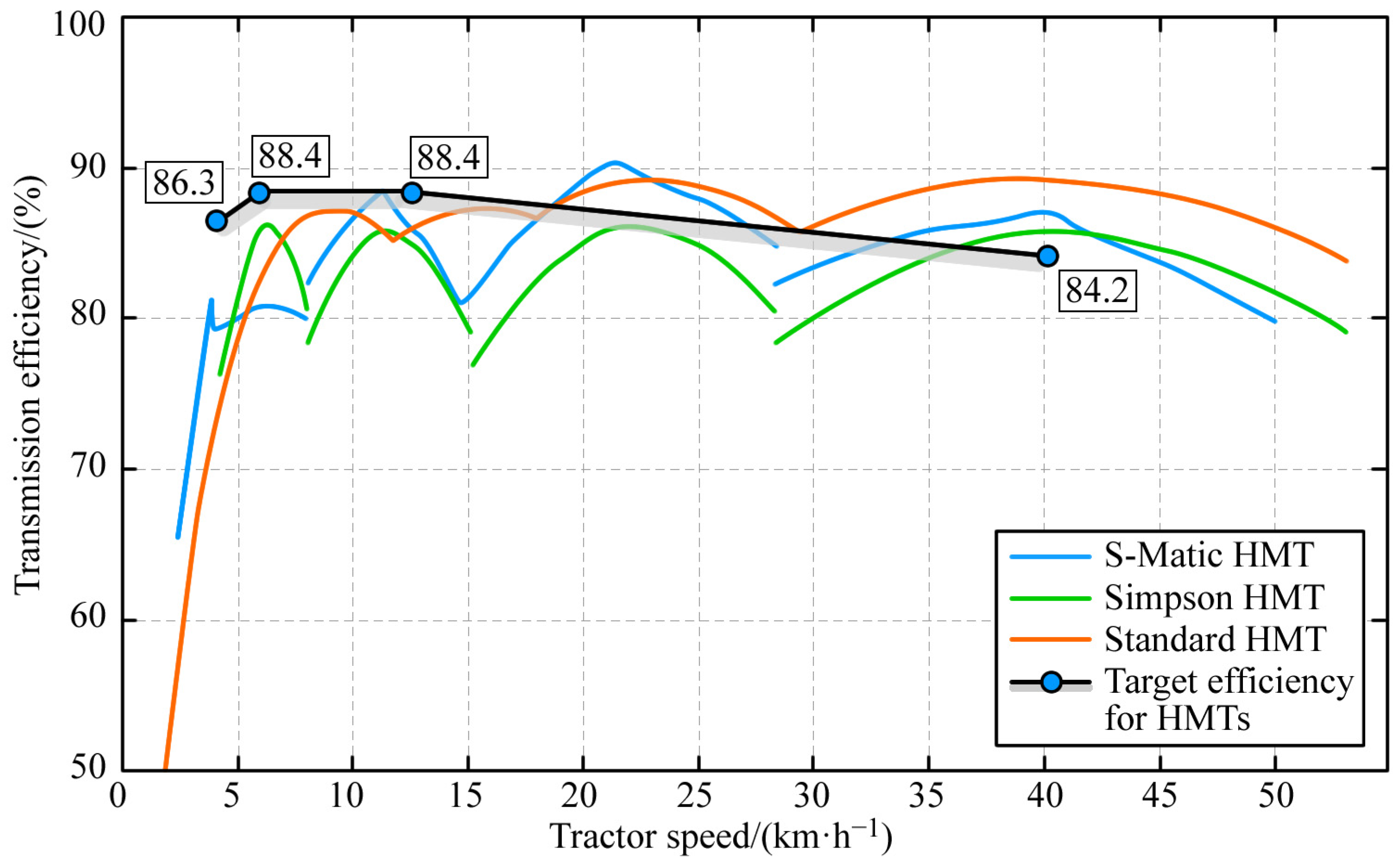
3.7. Further Comparison with Target Efficiency Proposed by Renius
Renius [22] proposed a target efficiency (engine to wheels) for tractor CVTs above 100 kW. Although few transmissions can meet this standard, it is still widely used to assess the performance of tractor HMTs. We assumed that the efficiency of the rear axle was 0.95, such that the target efficiency of the transmission system was converted into the efficiency of the HMT. We compared the efficiencies of the Standard HMT, the Simpson HMT, and S-Matic HMT (produced by ZF) with the target efficiency, and the results are shown in Figure 12. It shows that none of the three transmissions achieved Renius’s ideal target efficiency. The Simpson HMT had relatively low efficiency, but the changes in it were relatively stable. S-Matic had a higher efficiency in the third range than the other two transmissions but had an efficiency of only about 80% in the first range that could have increased its energy consumption for heavy-load operations, such as plowing. The efficiency of the Standard HMT was the closest to Renius’s target efficiency, and it recorded minimal fluctuations.
In summary, the HMT with a single planetary gear set proposed in this study has a higher efficiency of transmission and lower energy consumption than traditional HMTs. However, it still cannot attain Renius’s target efficiency, and its efficiency in the range RL in particular needs to be further optimized.
4. Conclusions
In this study, the authors analyzed the energy and fuel consumption of an HMT with a single planetary gear in comparison with the Simpson HMT. The main conclusions are as follows:
- The HMT had lower energy consumption at the rated engine speed, with efficiencies of 0–75%, 0–87%, and 75–89% in the ranges RY, RL, and RH, respectively, under a full load. Considering that the speed of the tractor once it had started was 4 km/h, the maximum portion of hydrostatic power of the HMT in each range was about 45–46%. When influenced by parasitic power, the efficiency of this HMT was higher when the displacement of the pump was positive than when it was negative. Reducing the engine speed and increasing the load-induced torque can both improve the efficiency of transmission of the HMT during operation. However, when the tractor moved at a low speed, an excessive load-induced torque could increase the loss of speed of the motor and reduce the efficiency of transmission of the HMT. Therefore, the hydrostatic power-split ranges of the HMT are not suitable for operation at extremely low speeds but can be used to start the tractor. This allows for the removal of the brake in the hydrostatic range to further simplify the structure of the transmission.
- The distribution of the fuel consumption of the system in the engine map was approximately consistent with that of the efficiency of the HMT, and both were centered around the optimal point of operation and expanded into nested rings. Therefore, the fuel consumption of the engine itself did not constrain the system’s fuel consumption, which caused the fuel economy of the tractor to be largely determined by the efficiency of transmission of the HMT.
- Compared with the Simpson HMT, the transmission examined here not only has a simpler structure and lower energy consumption but also has better fuel economy in most field operations. In this study, the fuel consumption of Standard HMT during plowing, harrowing, sowing, spraying, and field transportation is 0.8%, 1.4%, 16.5%, 3.3%, and 3.1% lower than that of Simpson HMT, respectively.
HMTs with a single planetary gear do not involve complex design-related issues related to the support and the uniform load structures that are caused by cascading multiple planetary gears. This significantly reduces the cost of their application. This study has demonstrated that the simple structure of the HMT examined here does not increase its energy and fuel consumption, and it even outperforms traditional HMTs in many operating conditions.
However, the process of the shift in the range of this HMT is complex and requires precise control of both the displacement of the pump and the status of the clutch. Based on this consideration, the authors think that this type of HMT is not suitable as a continuously variable transmission system for heavy-duty tractors but is suitable for use in large- and medium-sized tractors. In addition, it still cannot attain the target efficiency proposed by Renius, and its efficiency in the range RL is slightly lower than the ideal value. In future work, we plan to investigate the power-shift control of this HMT and further optimize its efficiency.
Author Contributions
Conceptualization, G.W. and Y.Z.; methodology, G.W. and Y.Z.; validation, G.W.; formal analysis, Y.Z. and X.C.; investigation, X.C. and Y.S.; resources, Y.S.; writing—original draft preparation, Y.Z. and X.C.; writing—review and editing, Y.Z., X.C. and Z.Z.; visualization, Y.Z. and X.C.; supervision, G.W.; project administration, G.W.; funding acquisition, G.W. All authors have read and agreed to the published version of the manuscript.
Funding
This research was funded by Shandong Provincial Natural Science Foundation, Grant Number ZR2020QE163, and Shandong Provincial Key Research and Development Program, Grant Number 2018GNC112008.
Institutional Review Board Statement
Not applicable.
Informed Consent Statement
Not applicable.
Data Availability Statement
The data presented in this study are available on request from the corresponding authors. The data are not publicly available due to ongoing research.
Conflicts of Interest
The authors declare no conflict of interest.
Nomenclature
| HMT | Hydro-mechanical transmission. | , | Coefficients of loss of energy of the pump shaft and the motor shaft due to friction, respectively. |
| Full load | The efficiency of transmission of the HMT when the torque of the input shaft reaches the external characteristic torque of the engine. | , | Torques of gear 1 and gear 2, respectively. [N·m] |
| Partial load | The efficiency of transmission of the HMT when the torque of the input shaft does not reach the external characteristic torque of the engine. | Efficiency of meshing of gear 1 and gear 2. | |
| Standard HMT | HMT with a single planetary gear. | , , | Torques of the sun gear, the ring gear, and the carrier, respectively. [N·m] |
| Simpson HMT | HMT with two single planetary gears. | Efficiency of transmission of the planetary gear. | |
| RY, RL, RH, RR | Ranges of the Standard planetary HMT. | , | Relative efficiencies of transmission of the sun gear and the planetary gears and of the ring gear and the planetary gears, respectively. |
| GL, GH | Mechanical gears of the Standard planetary HMT. | Speed of rotation of the planetary gears in the conversion mechanism. [r/min] | |
| HY, HM1–4 | Ranges of the Simpson planetary HMT. | Efficiency of transmission of the HMT. | |
| , | Theoretical flows of the pump and the motor, respectively. [L/min] | Output speed of the HMT. [r/min] | |
| , | Rated displacements of the pump and the motor, respectively. [m3/rad] | , | Torques of the engine and the output torque of the HMT, respectively. [N·m] |
| , | Speeds of rotation of the pump shaft and the motor shaft, respectively. [r/min] | , | Engine fuel consumption and system fuel consumption, respectively. [g/(kw·h)] |
| e | Ratio of displacement of the pump to that of the motor. | , | Portions of hydrostatic power of the HMT with and without parasitic power, respectively. |
| Leakage-induced flow of the hydraulic system. [L/min] | , , | Powers of the sun gear, the ring gear and the planet carrier, respectively. [kW] | |
| Total coefficient of leakage of hydraulic oil. | Traction resistance. [N] | ||
| Difference in pressure between the inlet and the outlet of the motor. [Pa] | Number of plowshares | ||
| Dynamic viscosity of hydraulic oil. [Pa·s] | , | The depth and the width of the plow, respectively. [cm] | |
| , | Speeds of rotation of gear 1 and gear 2. [r/min] | Soil-specific resistance of plowing. [N/cm2] | |
| Transmission ratio of gear 1 and gear 2. | Coefficient of utilization of traction. | ||
| , , | Speeds of rotation of the sun gear, the ring gear, and the carrier of the planetary gear set, respectively. [r/min] | , | The depth and the width of the harrow, respectively. [cm] |
| k | Standing ratio of the planetary gear set. | Soil-specific resistance of harrowing. [N/cm2] | |
| Transmission ratio of the tractor in the range (∈ {Y, L, H}). | Number of openers. | ||
| The gear pair gx (x = 1–6). | Working resistance of a single opener. [N] | ||
| Speed of the tractor. | Rolling resistance. [N] | ||
| Engine speed. [r/min] | , | Masses of the tractor and the agricultural machinery, respectively. [kg] | |
| Power radius of the driving wheel of the tractor. [m] | Ravitational acceleration. [m/s2] | ||
| Transmission ratio of the rear axle of the tractor. | Coefficient of rolling resistance. | ||
| , | Torques of the pump shaft and the motor shaft, respectively. [N·m] | Output power of the HMT. [kW] | |
| Coefficients of viscous damping of the pump shaft and the motor shaft, respectively. [N·m·s/rad] | Efficiency of the transmission of the rear axle. |
References
- Available online: https://data.stats.gov.cn (accessed on 30 May 2023).
- Han, J.Y.; Yan, X.X.; Tang, H. Method of controlling tillage depth for agricultural tractors considering engine load characteristics. Biosyst. Eng. 2023, 227, 95–106. [Google Scholar] [CrossRef]
- Ranjbarian, S.; Askari, M.; Jannatkhah, J. Performance of tractor and tillage implements in clay soil. J. Saudi Soc. Agric. Sci. 2017, 16, 154–162. [Google Scholar] [CrossRef] [Green Version]
- Buberger, J.; Kersten, A.; Kuder, M.; Eckerle, R.; Weyh, T.; Thiringer, T. Total CO2-equivalent life-cycle emissions from commercially available passenger cars. Renew. Sustain. Energy Rev. 2022, 159, 112158. [Google Scholar] [CrossRef]
- Edwards, R.; Hass, H.; Larivé, J.F.; Lonza, L.; Maas, H.; Rickeard, D. Well-to-Wheels Analysis of Future Automotive Fuels and Powertrains in the European Context; Technical Report by the Joint Research Centre of the European Commission; European Commission: Ispra, Italy, January 2014.
- Li, J.F.; Wu, X.H.; Zhang, X.M.; Song, Z.H.; Li, W.J. Design of distributed hybrid electric tractor based on axiomatic design and Extenics. Adv. Eng. Inform. 2022, 54, 101765. [Google Scholar] [CrossRef]
- Chen, Y.N.; Xie, B.; Du, Y.X.; Mao, E.R. Powertrain parameter matching and optimal design of dual-motor driven electric tractor. Int. J. Agric. Biol. Eng. 2019, 12, 33–41. [Google Scholar] [CrossRef] [Green Version]
- Chen, Y.C.; Chen, L.W.; Chang, M.Y. A design of an unmanned electric tractor platform. Agriculture 2022, 12, 112. [Google Scholar] [CrossRef]
- Zhang, Q.; Sun, D.Y.; Qin, D.T. Optimal parameters design method for power reflux hydro-mechanical transmission system. Proc. Inst. Mech. Eng. Part D 2019, 233, 585–594. [Google Scholar] [CrossRef]
- Xue, L.J.; Jiang, H.H.; Zhao, Y.H.; Wang, J.B.; Wang, G.M.; Xiao, M.H. Fault diagnosis of wet clutch control system of tractor hydrostatic power split continuously variable transmission. Comput. Electron. Agric. 2022, 194, 106778. [Google Scholar] [CrossRef]
- Yu, J.; Cao, Z.; Cheng, M.; Pan, R.Z. Hydro-mechanical power split transmissions: Progress evolution and future trends. Proc. Inst. Mech. Eng. Part D 2019, 233, 727–739. [Google Scholar] [CrossRef]
- Nilsson, T.; Fröberg, A.; Åslund, J. Fuel potential and prediction sensitivity of a power-split CVT in a wheel loader. In Proceedings of the 2012 Workshop on Engine and Powertrain Control, Simulation and Modeling, Rueil-Malmaison, France, 23–25 October 2012. [Google Scholar]
- Ince, E.; Guler, M.A. On the advantages of the new power-split infinitely variable transmission over conventional mechanical transmissions based on fuel consumption analysis. J. Clean. Prod. 2020, 244, 118795. [Google Scholar] [CrossRef]
- Rossetti, A.; Macor, A.; Benato, A. Impact of control strategies on the emissions in a city bus equipped with power-split transmission. Transp. Res. D Transp. Environ. 2017, 50, 357–371. [Google Scholar] [CrossRef]
- Wang, G.M.; Zhao, Y.H.; Song, Y.; Xue, L.J.; Chen, X.H. Optimizing the fuel economy of hydrostatic power-split system in continuously variable tractor transmission. Heliyon 2023, 9, e15915. [Google Scholar] [CrossRef]
- Rossetti, A.; Macor, A. Control strategies for a powertrain with hydromechanical transmission. Energy Procedia 2018, 148, 978–985. [Google Scholar] [CrossRef]
- Ahn, S.; Choi, J.; Kim, S.; Lee, J.; Choi, C.; Kim, H. Development of an integrated engine-hydro-mechanical transmission control algorithm for a tractor. Adv. Mech. Eng. 2015, 7, 1687814015593870. [Google Scholar] [CrossRef]
- Liu, H.X.; Han, L.; Cao, Y. Improving transmission efficiency and reducing energy consumption with automotive continuously variable transmission: A model prediction comprehensive optimization approach. Appl. Energy 2020, 274, 115303. [Google Scholar] [CrossRef]
- Mola, M.; Amani, A.M.; Jalili, M.; Khayyam, H. Data-Driven Predictive Control of CVT System for Improving Energy Efficiency of Autonomous Vehicles. IEEE Trans. Veh. Technol. 2023, 72, 1501–1514. [Google Scholar] [CrossRef]
- Fu, B.; Zhu, T.P.; Liu, J.G.; Zhao, Y.H.; Chen, J.W. Influencing Factors of Electric Vehicle Economy Based on Continuously Variable Transmission. Int. J. Automot. Technol. 2022, 23, 717–728. [Google Scholar] [CrossRef]
- Zhang, M.Z.; Wang, J.Z.; Wang, J.H.; Guo, Z.Z.; Guo, F.Q.; Xi, Z.Q.; Xu, J.J. Speed changing control strategy for improving tractor fuel economy. Trans. Chin. Soc. Agric. Eng. 2020, 36, 82–89. [Google Scholar] [CrossRef]
- Renius, K.T.; Resch, R. Continuously variable tractor transmissions. In Proceedings of the 2005 Agricultural Equipment Technology Conference, Louisville, KY, USA, 14–16 February 2005. [Google Scholar]
- Rossetti, A.; Macor, A. Multi-objective optimization of hydro-mechanical power split transmissions. Mech. Mach. Theory 2013, 62, 112–128. [Google Scholar] [CrossRef]
- Rossetti, A.; Macor, A.; Scamperle, M. Optimization of components and layouts of hydromechanical transmissions. Int. J. Fluid Power 2017, 18, 123–134. [Google Scholar] [CrossRef]
- Xia, Y.; Sun, D.Y.; Qin, D.T.; Zhou, X.Y. Optimisation of the power-cycle hydro-mechanical parameters in a continuously variable transmission designed for agricultural tractors. Biosyst. Eng. 2020, 193, 12–24. [Google Scholar] [CrossRef]
- Ince, E.; Güler, M.A. Design and analysis of a novel power-split infinitely variable power transmission system. J. Mech. Des. 2019, 141, 54501. [Google Scholar] [CrossRef]
- Nao, Z.G. Introduction to planetary gear transmission. In Design of Planetary Gear Transmission, 2nd ed.; Zhang, X.H., Yan, M., Eds.; Chemical Industry Press: Beijing, China, 2019. [Google Scholar]
- Wang, G.M.; Song, Y.; Wang, J.B.; Xiao, M.H.; Cao, Y.L.; Chen, W.Q.; Wang, J.X. Shift quality of tractors fitted with hydrostatic power split CVT during starting. Biosyst. Eng. 2020, 196, 183–201. [Google Scholar] [CrossRef]
- Liu, F.X.; Wu, W.; Hu, J.B.; Yuan, S.H. Design of multi-range hydro-mechanical transmission using modular method. Mech. Syst. Signal Process. 2019, 126, 1–20. [Google Scholar] [CrossRef]
- Chen, W.Q.; Xu, Z.Y.; Wu, Y.Q.; Zhao, Y.H.; Wang, G.M.; Xiao, M.H. Analysis of the shift quality of a hydrostatic power split continuously variable cotton picker. Mech. Sci. 2021, 12, 589–601. [Google Scholar] [CrossRef]
- Guo, Z.Z.; Yuan, S.H.; Jing, C.B.; Wei, C. Modeling and simulation of shifting process in hydraulic machinery stepless transmission based on AMESim. Trans. Chin. Soc. Agric. Eng. 2009, 25, 86–91. [Google Scholar] [CrossRef]
- Leitner, J.; Aitzetmüller, H.; Marzy, R. Das mechanisch-hydrostatisch leistungsverzweigte, stufenlose Fahrzeuggetriebe S-Matic. In Proceedings of the Congress Antriebstechnik Zahnradgetriebe, Dresden, Germany, 14–15 September 2000. [Google Scholar]
Figure 1.
Powertrain of hydrostatic power-split transmission: (a) Standard HMT. (b) Simpson HMT.
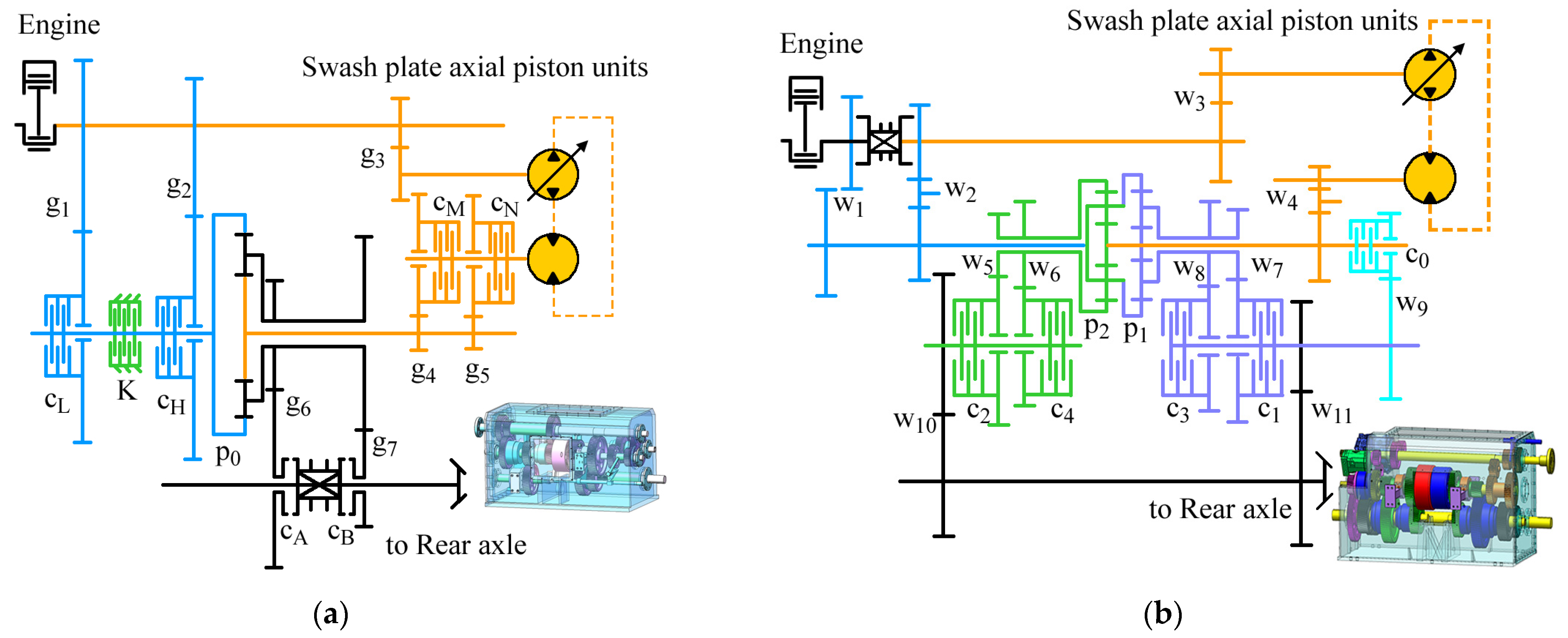
Figure 2.
Model to calculate the speed and torque of each HMT shaft.
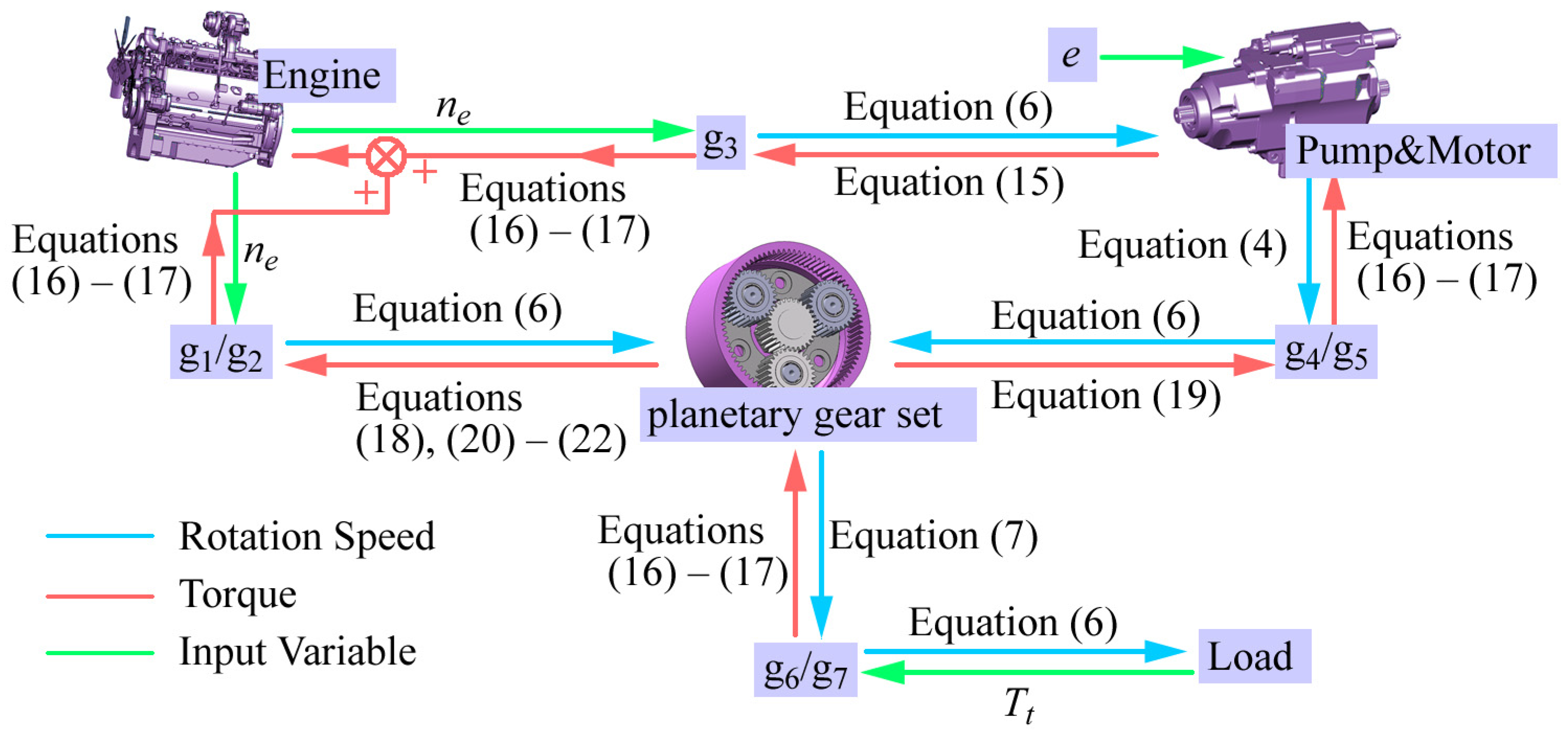
Figure 3.
Flowchart to calculate the energy and fuel consumption of HMT. Note: is the specified torque of the engine. is a function that solves the fuel consumption corresponding to the speed ne and the torque in the engine map.
Figure 3.
Flowchart to calculate the energy and fuel consumption of HMT. Note: is the specified torque of the engine. is a function that solves the fuel consumption corresponding to the speed ne and the torque in the engine map.
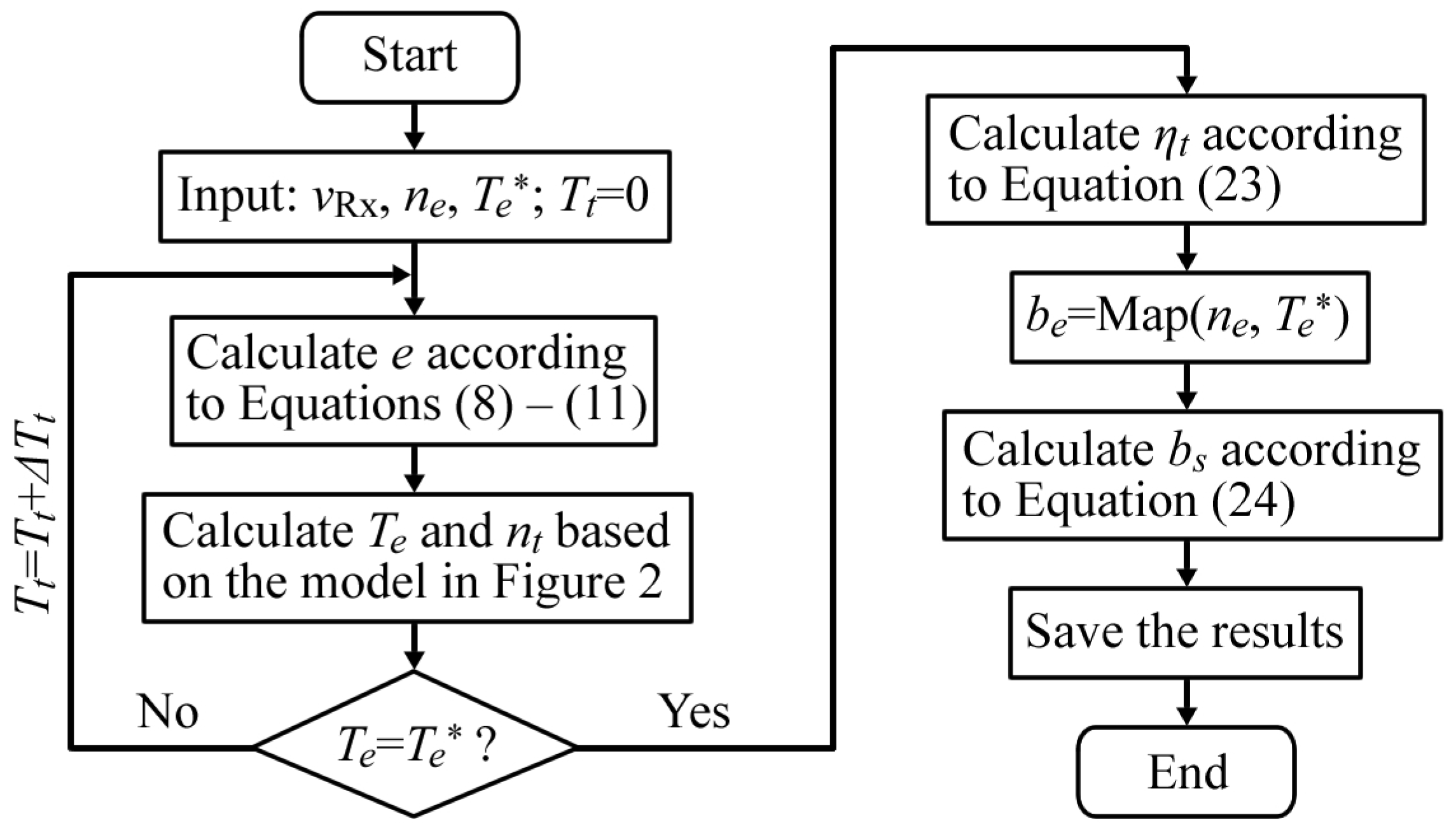
Figure 4.
Validation of methods of modeling based on the Simpson HMT (reproduced from [15]).
Figure 4.
Validation of methods of modeling based on the Simpson HMT (reproduced from [15]).
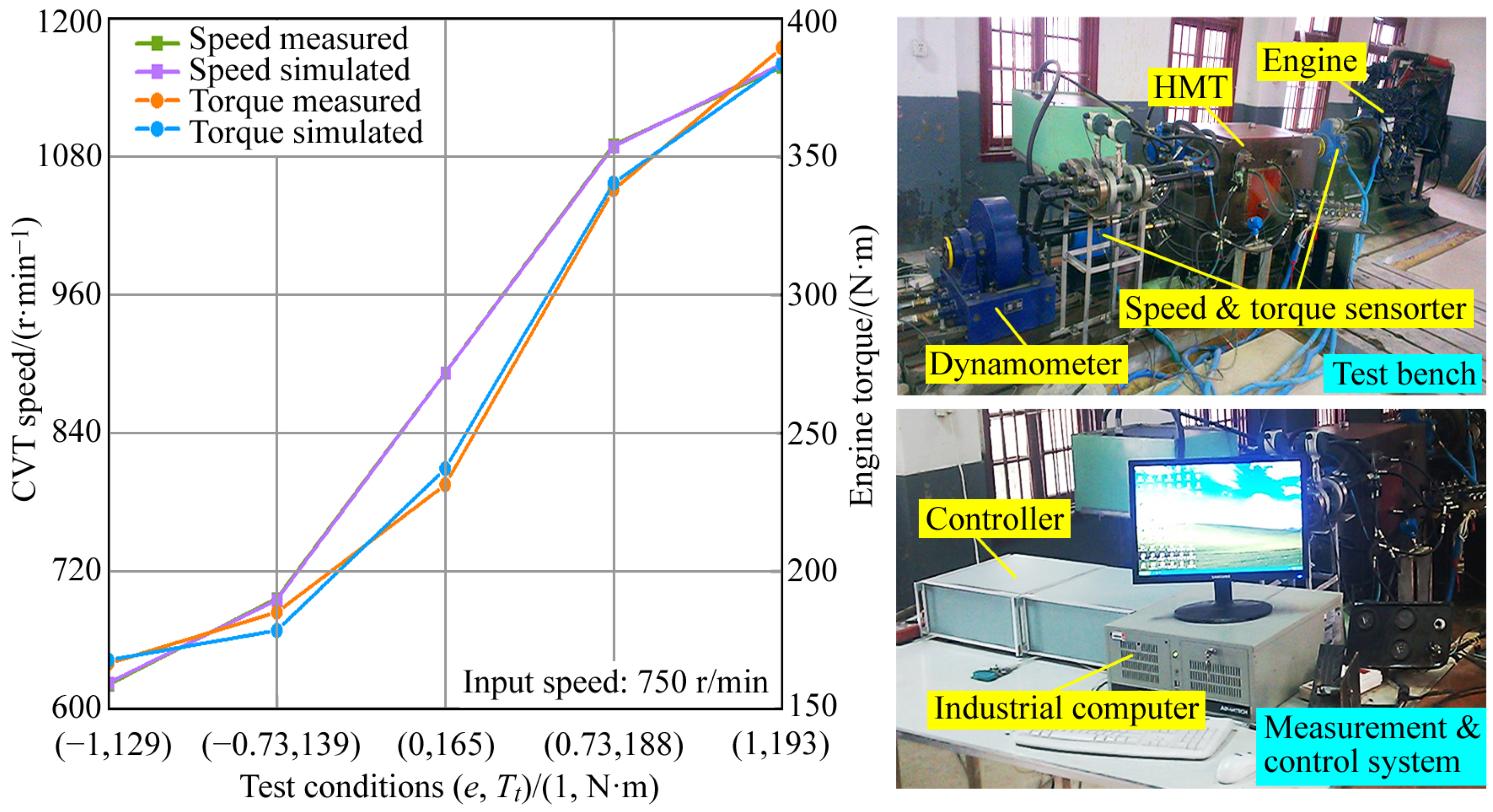
Figure 5.
Analysis of the flow of power of the transmission. Note: ① n is the rotational speed of the shaft, r/min; T is its torque, N·m; and P is its power, kW. ② “+” represents the counterclockwise direction, and “−” represents the clockwise direction. ③ When the speed and torque are in the same direction, the power is positive (denoted by ) and is otherwise negative (denoted by ). ④ Inside the planetary gear, power can flow only from the positive port to the negative port.
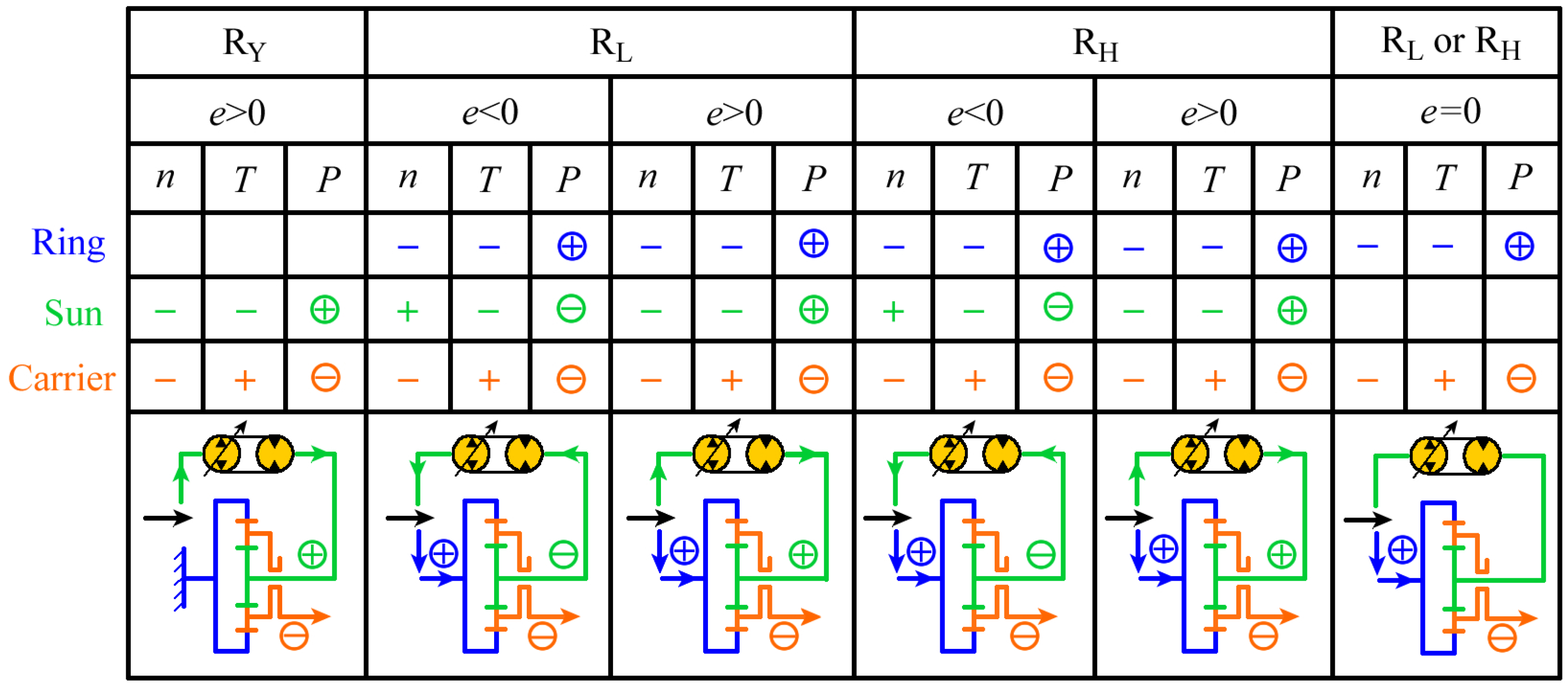
Figure 6.
Results of calculation of the portion of hydrostatic power.
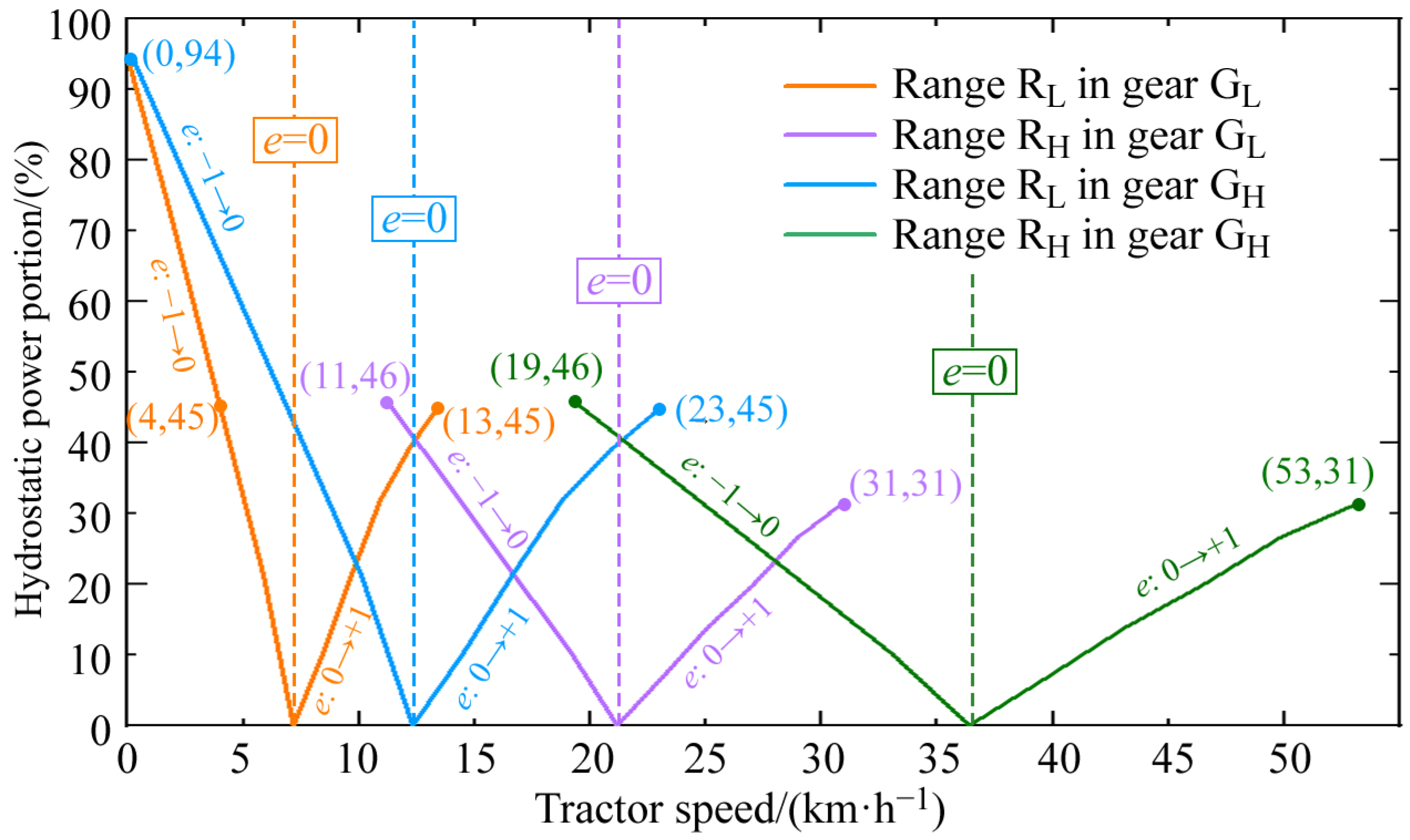
Figure 7.
Efficiency of transmission of the HMT under a full load.

Figure 8.
Efficiency map of the HMT at different tractor speeds: (a) Efficiency map of the HMT at 4 km/h. (b) Efficiency map of the HMT at 6 km/h. (c) Efficiency map of the HMT at 8 km/h. (d) Efficiency map of the HMT at 10 km/h. (e) Efficiency map of the HMT at 12 km/h. (f) Efficiency map of the HMT at 14 km/h. (g) Efficiency map of the HMT at 16 km/h. (h) Efficiency map of the HMT at 18 km/h. Note: When the engine speed dropped below a certain threshold, the specified tractor speed could not be achieved because the displacement of the pump was adjusted to its maximum value. The engine speed below this threshold is defined as “invalid engine speed” in this study.
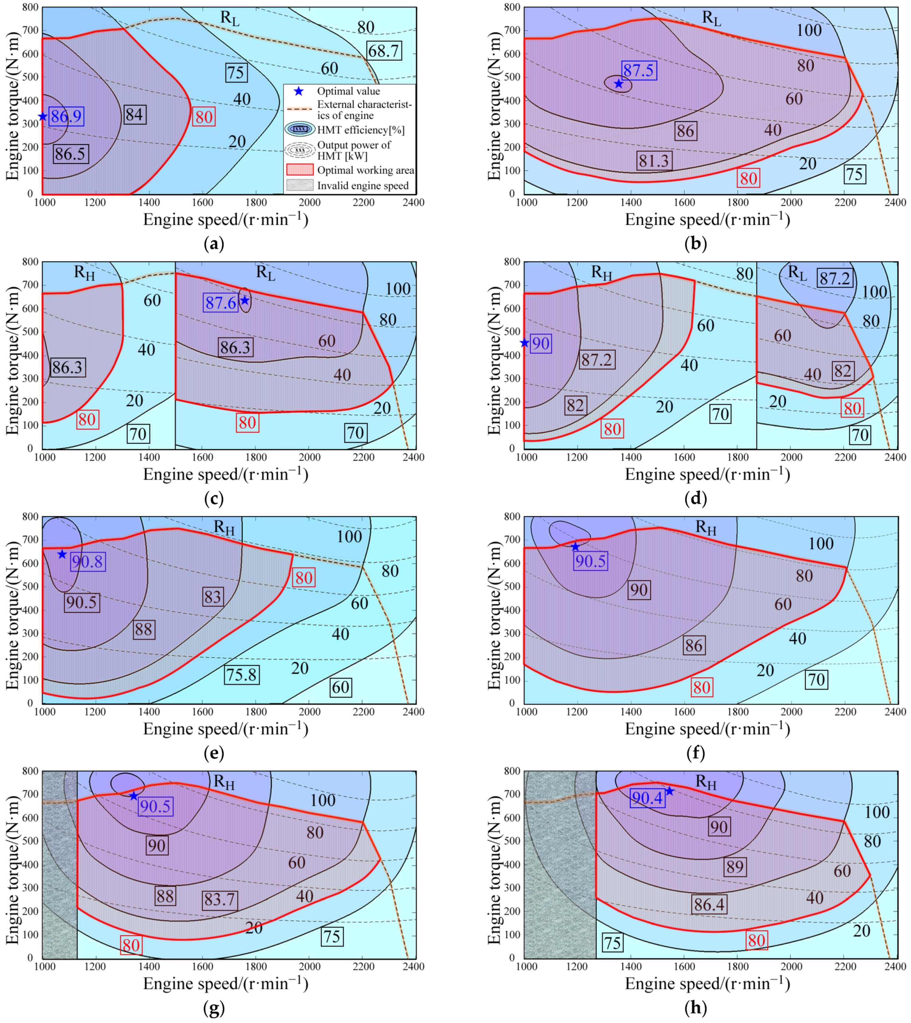
Figure 9.
Map of fuel consumption of the HMT at different tractor speeds: (a) Map of fuel consumption of the HMT at 4 km/h. (b) Map of fuel consumption of the HMT at 6 km/h. (c) Map of fuel consumption of the HMT at 8 km/h. (d) Map of fuel consumption of the HMT at 10 km/h. (e) Map of fuel consumption of the HMT at 12 km/h. (f) Map of fuel consumption of the HMT at 14 km/h. (g) Map of fuel consumption of the HMT at 16 km/h. (h) Map of fuel consumption of the HMT at 18 km/h.

Figure 10.
Energy and fuel consumption of the Simpson HMT: (a) Efficiency of the Simpson HMT under a full load. (b) Efficiency map of the Simpson HMT at 8 km/h. (c) Map of fuel consumption of the Simpson HMT at a speed of 8 km/h.
Figure 10.
Energy and fuel consumption of the Simpson HMT: (a) Efficiency of the Simpson HMT under a full load. (b) Efficiency map of the Simpson HMT at 8 km/h. (c) Map of fuel consumption of the Simpson HMT at a speed of 8 km/h.
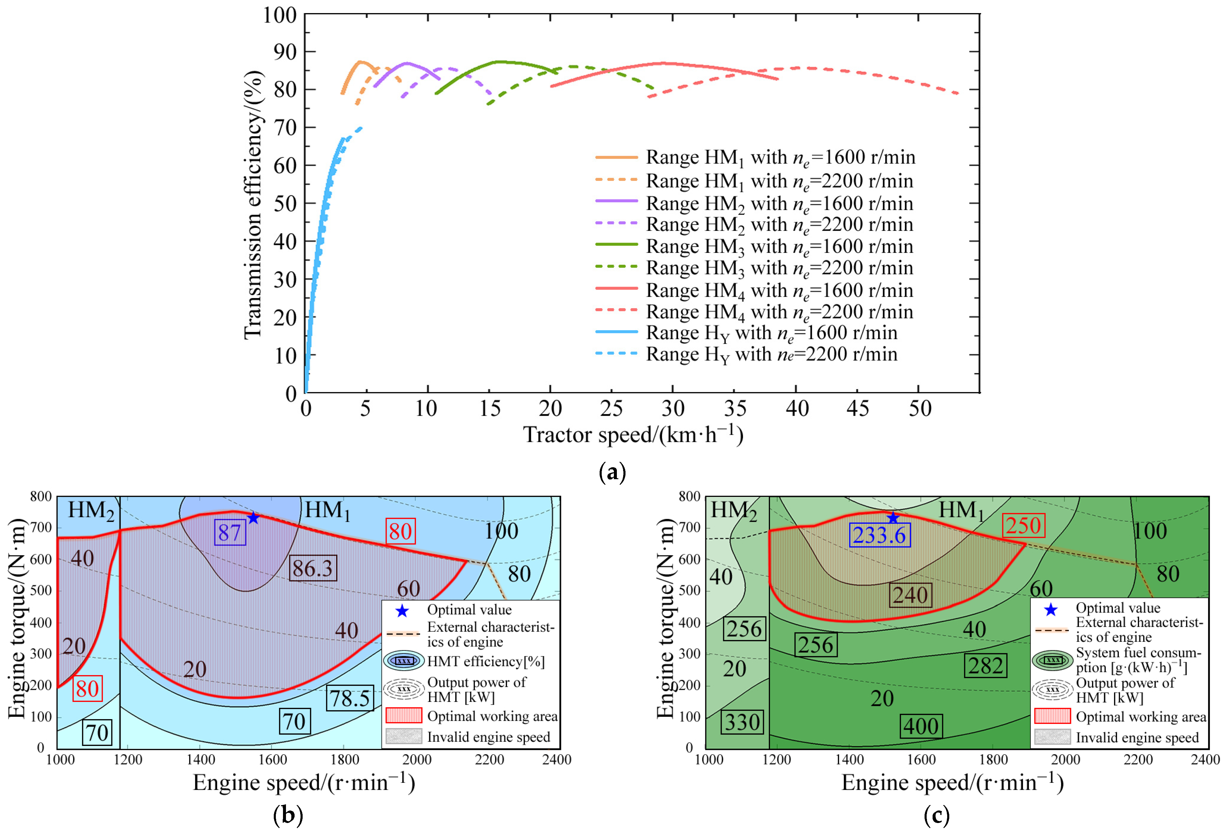
Figure 11.
The minimum fuel consumption of the two HMTs under various operating conditions: (a) The minimum fuel consumption of the Standard HMT under various operating conditions. (b) The minimum fuel consumption of the Simpson HMT under various operating conditions. (c) Comparison of fuel consumption between two HMTs under various operating conditions.
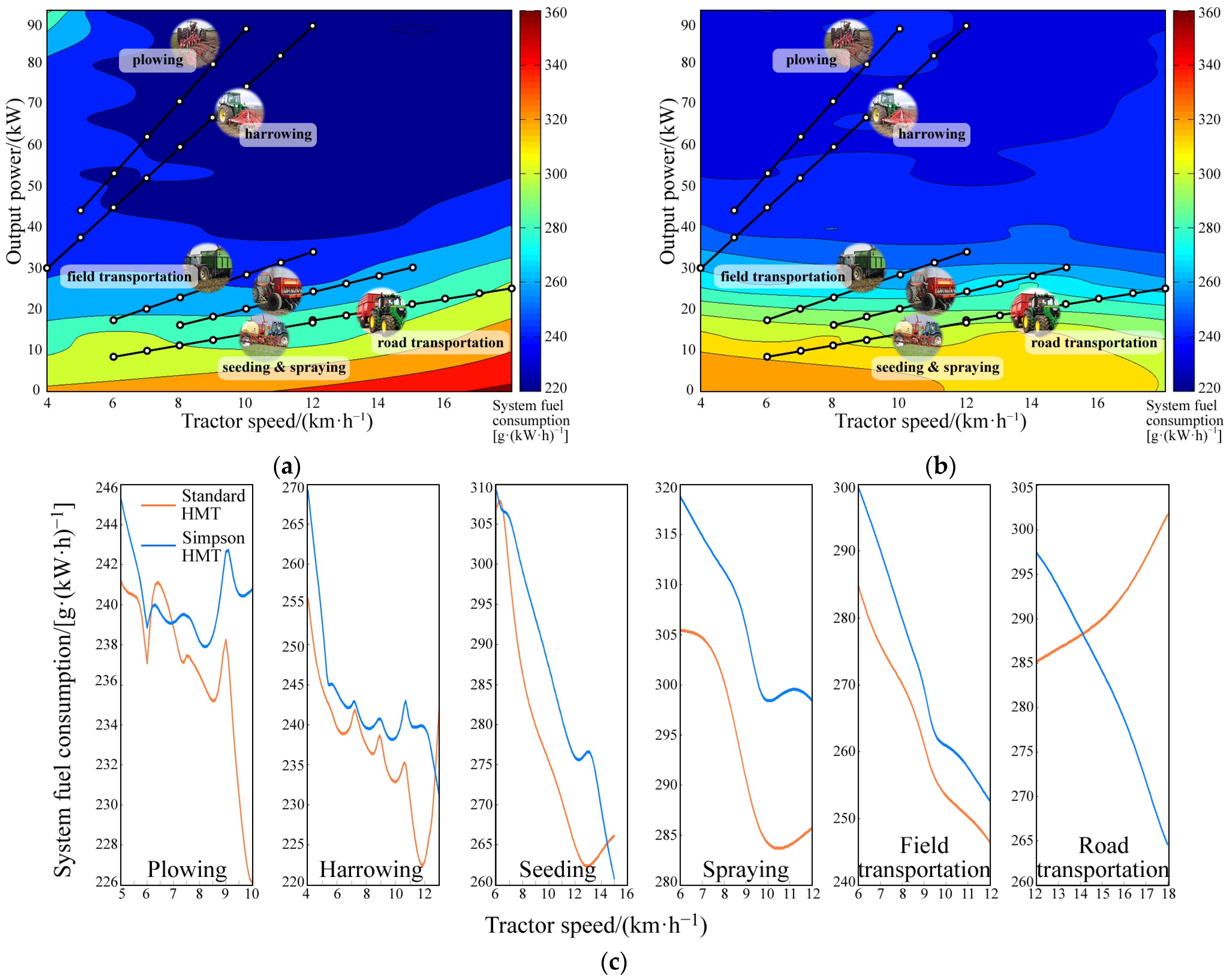
Figure 12.
Differences between the efficiencies of various HMTs under a full load and the target efficiency proposed by Renius. Note: ① S-Matic has been applied to the New Holland TVT tractor series, and data on its efficiency have been published by Leitner et al. [32]. ② The efficiencies of each gear and range of the Standard HMT in the figure have been merged.

Table 1.
Clutch and brake schedules of the Standard HMT.
| Gear | Range | Clutch/Brake | Planetary Gear | ||||||
|---|---|---|---|---|---|---|---|---|---|
| cL | cH | cM | cN | cA | cB | K | p0 | ||
| GL | RY | ○ | ○ | ● | ○ | ● | ○ | ● | ● |
| RL | ● | ○ | ● | ○ | ● | ○ | ○ | ● | |
| RH | ○ | ● | ○ | ● | ● | ○ | ○ | ● | |
| RR | ○ | ○ | ○ | ● | ● | ○ | ● | ● | |
| GH | RY | ○ | ○ | ● | ○ | ○ | ● | ● | ● |
| RL | ● | ○ | ● | ○ | ○ | ● | ○ | ● | |
| RH | ○ | ● | ○ | ● | ○ | ● | ○ | ● | |
| RR | ○ | ○ | ○ | ● | ○ | ● | ● | ● | |
Note: ● The clutch is engaged, or the planetary gear transmits torque. ○ The clutch is separated, or the planetary gear rotates freely.
Table 2.
Clutch and planetary gear schedules of the Simpson HMT.
| Range | Clutch | Planetary Gear | |||||
|---|---|---|---|---|---|---|---|
| c0 | c1 | c2 | c3 | c4 | p1 | p2 | |
| HY | ● | ○ | ○ | ○ | ○ | ○ | ○ |
| HM1 | ○ | ● | ○ | ○ | ○ | ● | ○ |
| HM2 | ○ | ○ | ● | ○ | ○ | ○ | ● |
| HM3 | ○ | ○ | ○ | ● | ○ | ● | ○ |
| HM4 | ○ | ○ | ○ | ○ | ● | ○ | ● |
Note: ● The clutch is engaged, or the planetary gear transmits torque. ○ The clutch is separated, or the planetary gear rotates freely.
Table 3.
Fuel consumption of HMT at intermediate speeds under various operating conditions [g/(kW·h)].
Table 3.
Fuel consumption of HMT at intermediate speeds under various operating conditions [g/(kW·h)].
| Plowing | Harrowing | Seeding | Spraying | Field Transportation | Road Transportation | |
|---|---|---|---|---|---|---|
| Simpson HMT | 239.5 | 239.8 | 284 | 300.5 | 269.4 | 284.1 |
| Standard HMT | 237.5 | 236.4 | 237.1 | 290.5 | 261 | 290 |
| Relative error (%) | 0.8 | 1.4 | 16.5 | 3.3 | 3.1 | −2.1 |
Disclaimer/Publisher’s Note: The statements, opinions and data contained in all publications are solely those of the individual author(s) and contributor(s) and not of MDPI and/or the editor(s). MDPI and/or the editor(s) disclaim responsibility for any injury to people or property resulting from any ideas, methods, instructions or products referred to in the content. |
© 2023 by the authors. Licensee MDPI, Basel, Switzerland. This article is an open access article distributed under the terms and conditions of the Creative Commons Attribution (CC BY) license (https://creativecommons.org/licenses/by/4.0/).
Share and Cite
MDPI and ACS Style
Zhao, Y.; Chen, X.; Song, Y.; Wang, G.; Zhai, Z. Energy and Fuel Consumption of a New Concept of Hydro-Mechanical Tractor Transmission. Sustainability 2023, 15, 10809. https://doi.org/10.3390/su151410809
AMA Style
Zhao Y, Chen X, Song Y, Wang G, Zhai Z. Energy and Fuel Consumption of a New Concept of Hydro-Mechanical Tractor Transmission. Sustainability. 2023; 15(14):10809. https://doi.org/10.3390/su151410809
Chicago/Turabian StyleZhao, Yehui, Xiaohan Chen, Yue Song, Guangming Wang, and Zhiqiang Zhai. 2023. "Energy and Fuel Consumption of a New Concept of Hydro-Mechanical Tractor Transmission" Sustainability 15, no. 14: 10809. https://doi.org/10.3390/su151410809
Note that from the first issue of 2016, this journal uses article numbers instead of page numbers. See further details here.