
Finding Patterns of Construction Systems in Low-Income Housing for Thermal and Energy Performance Evaluation through Cluster Analysis

Abstract
:1. Introduction
2. Background
2.1. Reference Models for Thermal and Energy Simulations
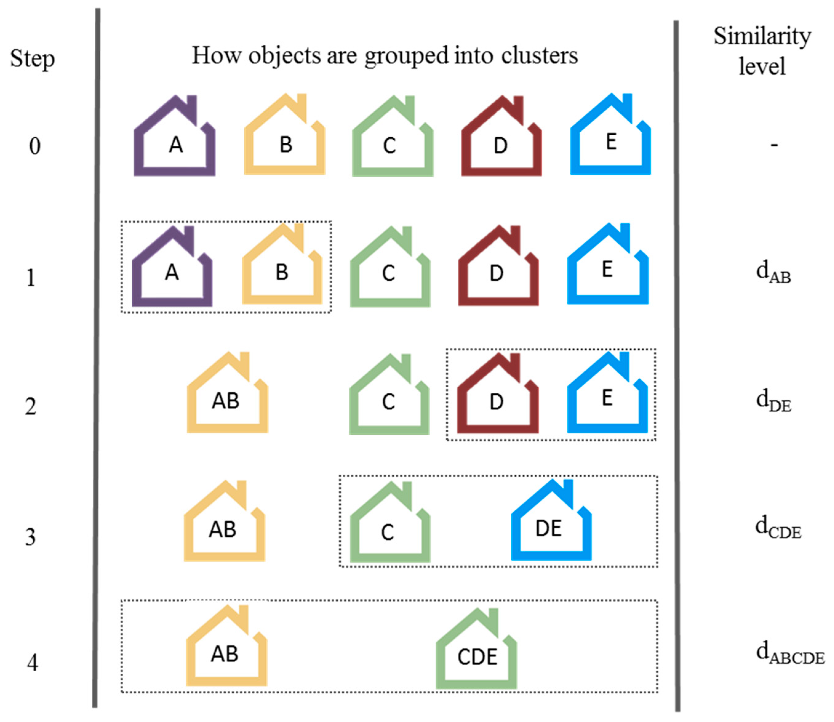
2.2. Cluster Analysis to Determine Reference Models
3. Method
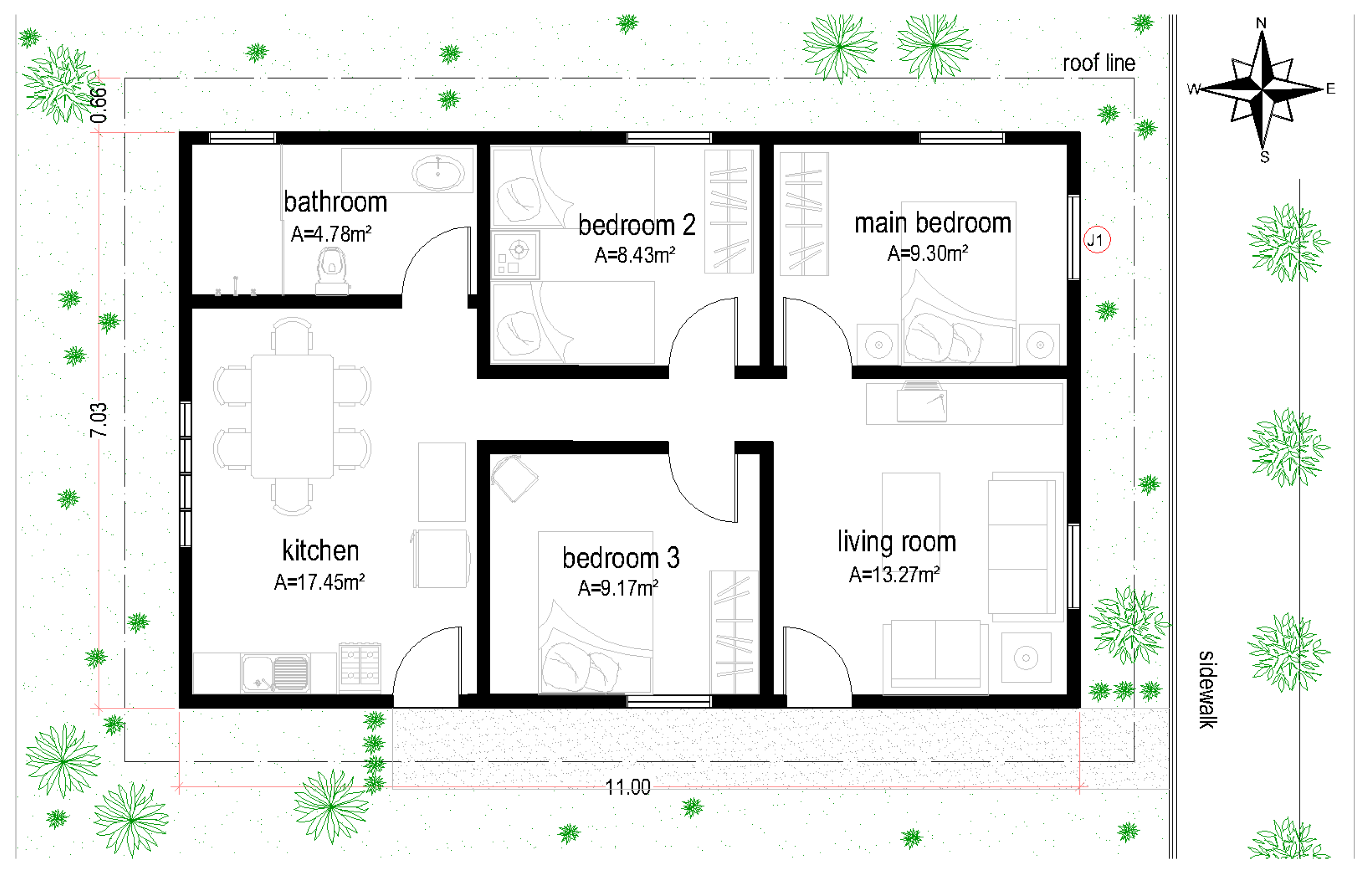
3.1. Obtaining Data
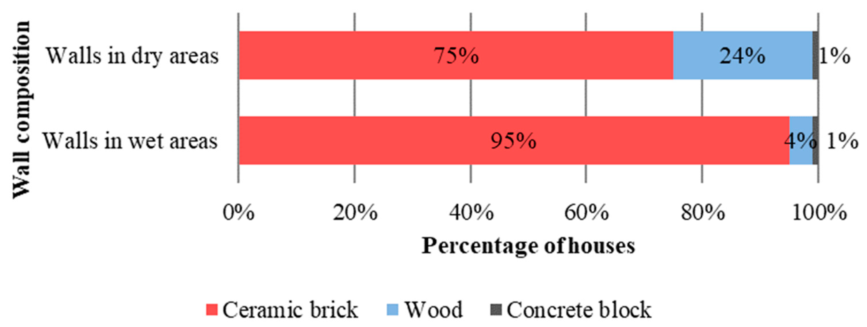
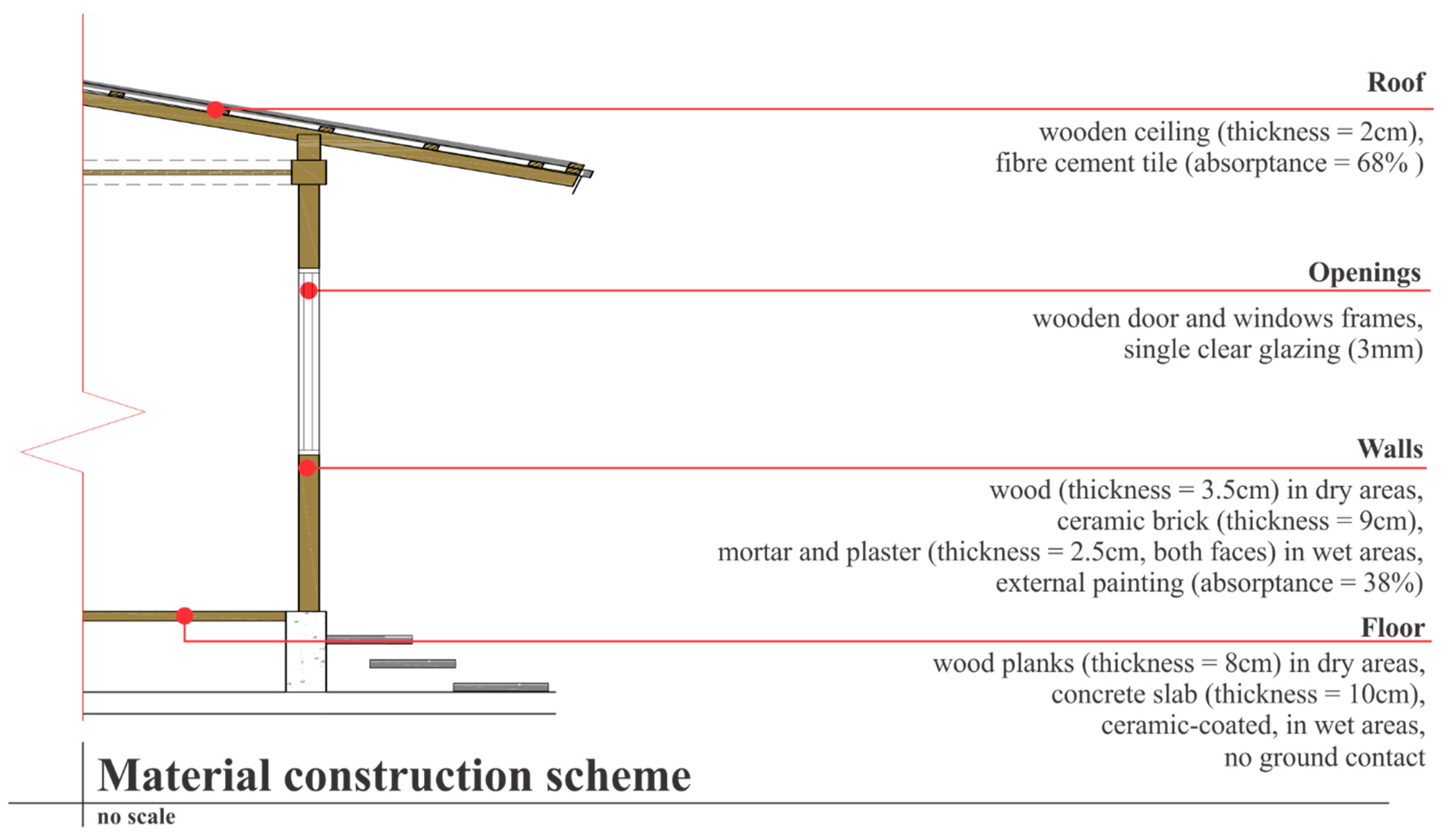
- Walls: thickness and materials that compose the wall, plaster, mortar, ceramic-brick or concrete block, wood, etc.;
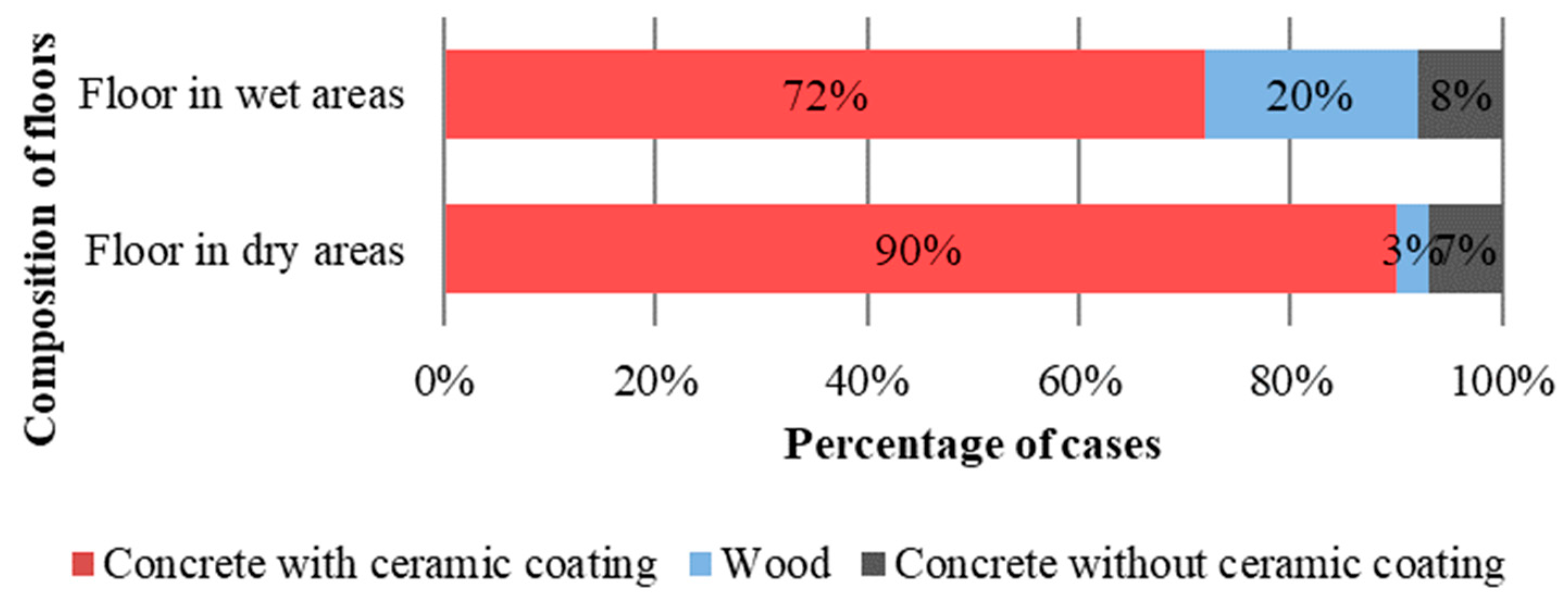
- Floor: floor covering, structure and contact or not with the ground;
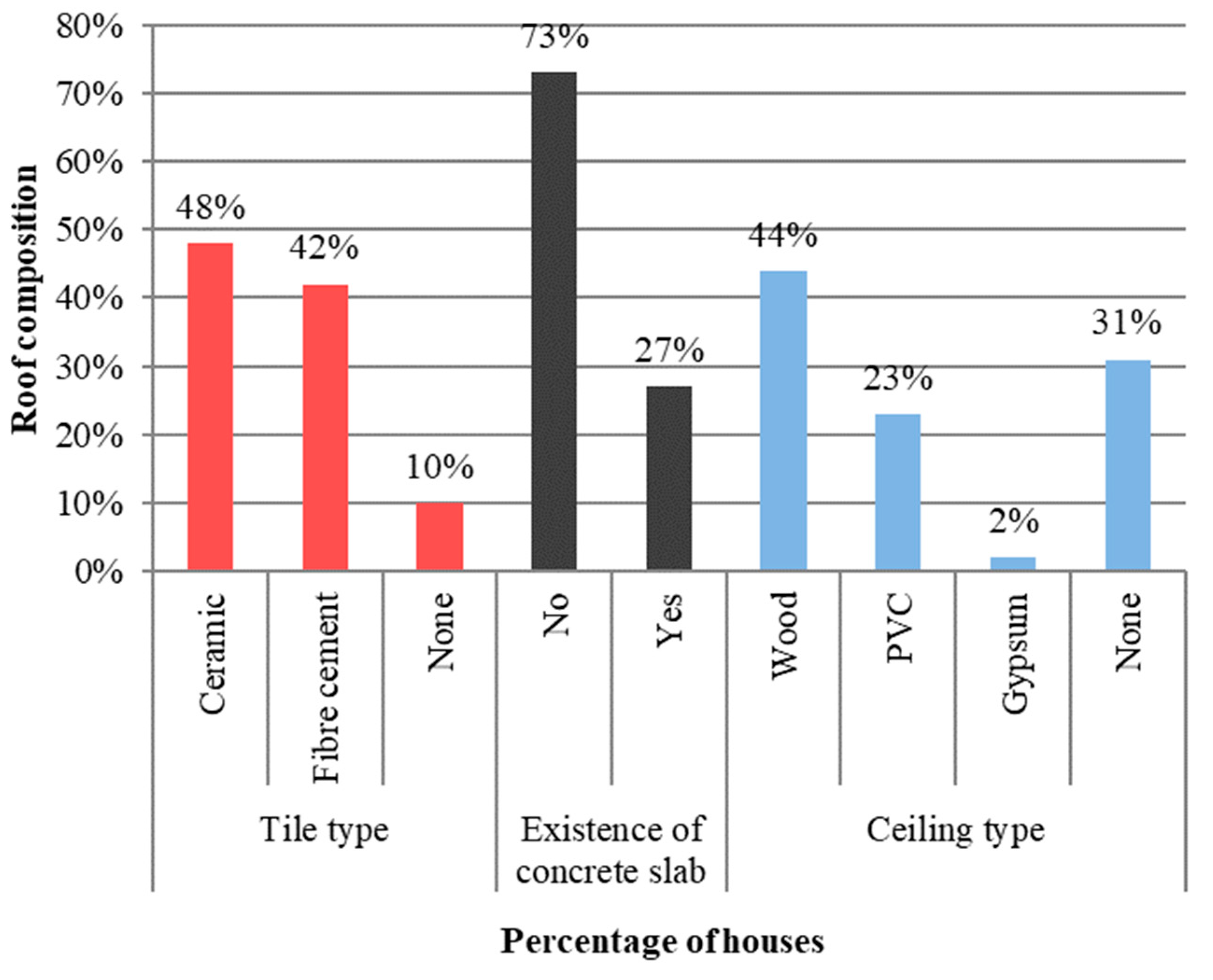
- Roof: type of tile, existence or not of a concrete slab and ceiling material, when applicable;
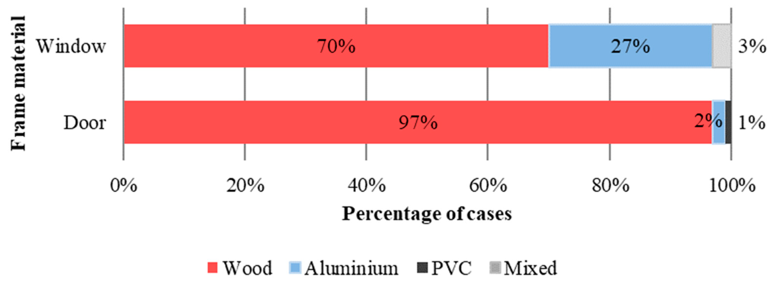
- Frames: frame material.
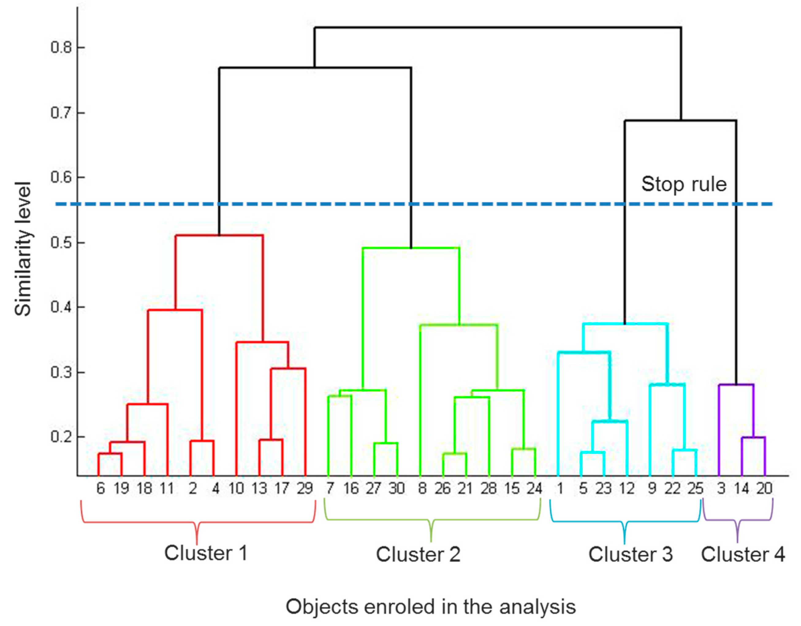
3.2. Cluster Analysis
3.3. Thermal Performance through Computer Simulation
4. Results and Discussion
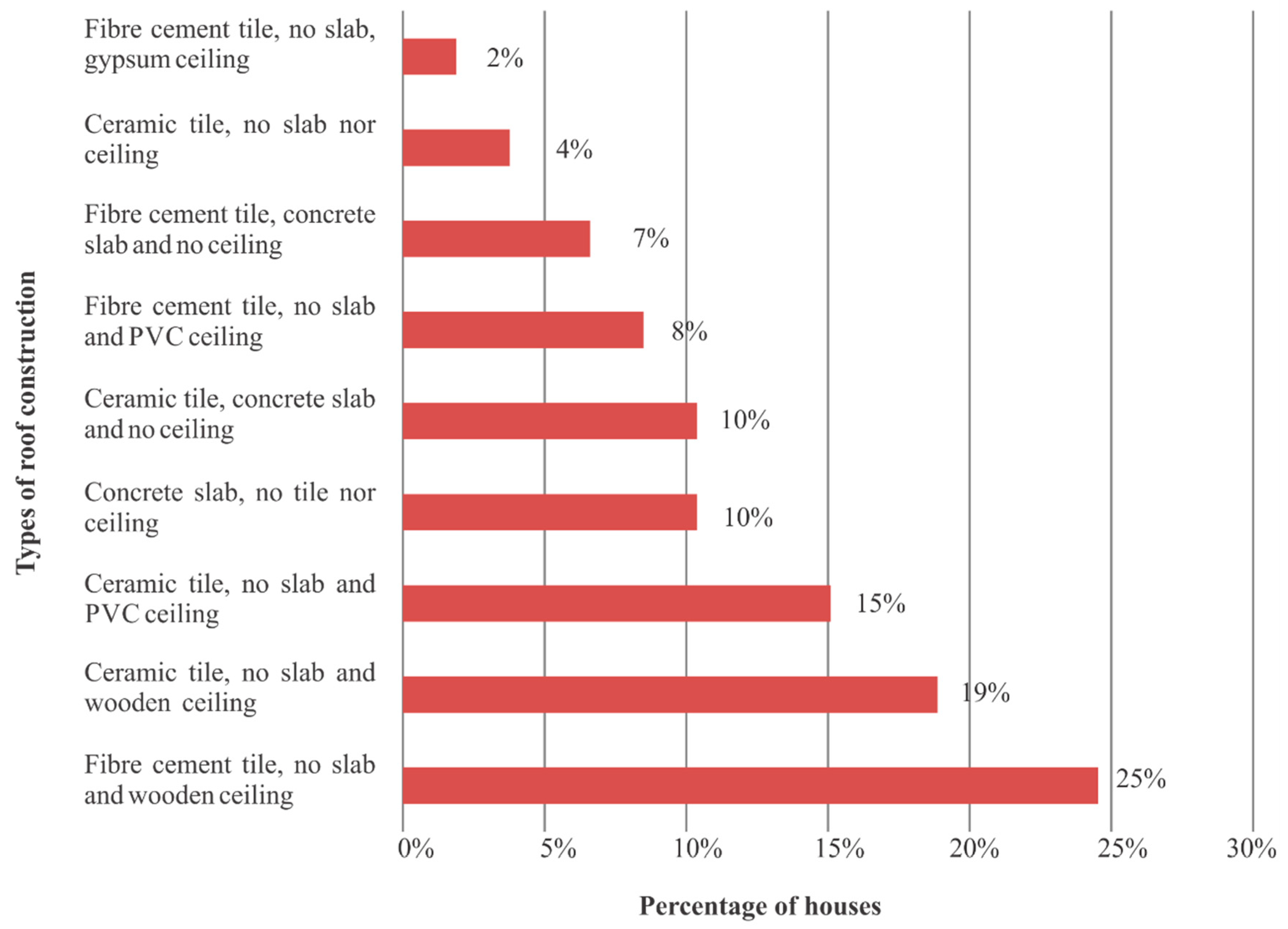
4.1. Data on Materials and Construction Systems
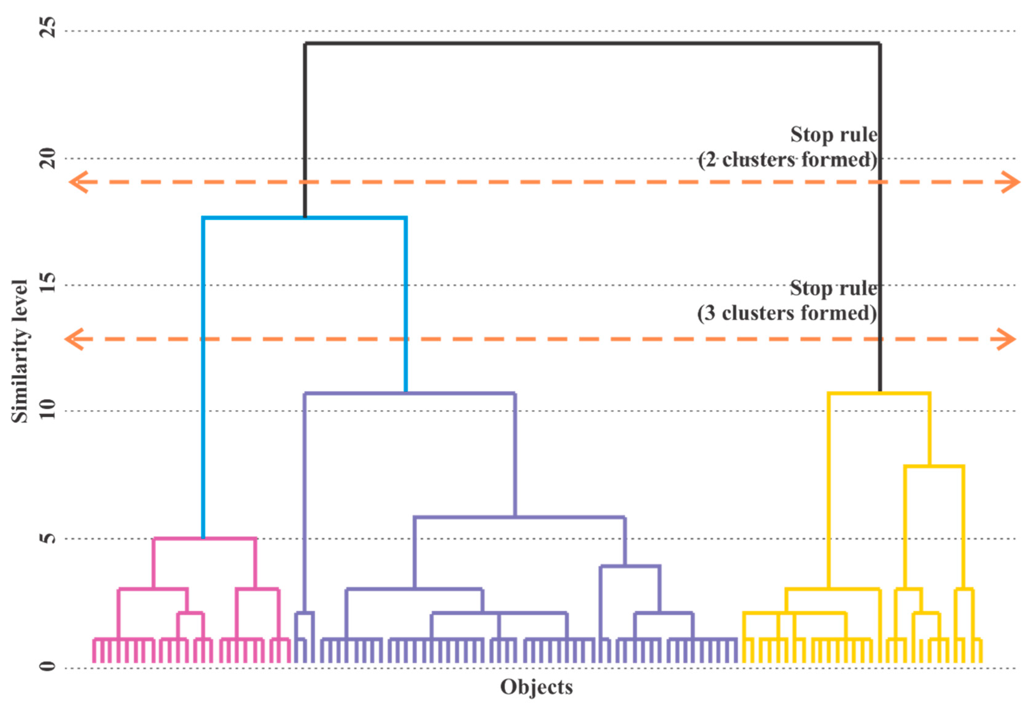
4.2. Clusters
4.3. Suitability of the Clusters and Their Reference Models Based on Thermal Performance
5. Conclusions
Author Contributions
Funding
Conflicts of Interest
References
- Fundação João Pinheiro. Déficit Habitacional No Brasil Por Cor Ou Raça (2016–2019); Fundação João Pinheiro: Brasília, Brazil, 2022. (In Portuguese) [Google Scholar]
- International Energy Agency. World Energy Outlook 2022; International Energy Agency: Paris, France, 2022. [Google Scholar]
- Empresa de Pesquisa Energética. Balanço Energético Nacional: Ano Base 2021; Empresa de Pesquisa Energética: Brasília, Brazil, 2022. (In Portuguese) [Google Scholar]
- Mousavi, S.N.; Gheibi, M.; Wacławek, S.; Smith, N.R.; Hajiaghaei-Keshteli, M.; Behzadian, K. Low-energy residential building optimisation for energy and comfort enhancement in semi-arid climate conditions. Energy Convers. Manag. 2023, 291, 117264. [Google Scholar] [CrossRef]
- Alaidroos, A.; Krarti, M. Optimal design of residential building envelope systems in the Kingdom of Saudi Arabia. Energy Build. 2015, 86, 104–117. [Google Scholar] [CrossRef]
- Yong, S.G.; Kim, J.H.; Gim, Y.; Kim, J.; Cho, J.; Hong, H.; Baik, Y.J.; Koo, J. Impacts of building envelope design factors upon energy loads and their optimization in US standard climate zones using experimental design. Energy Build. 2017, 141, 1–15. [Google Scholar] [CrossRef]
- Yousefi, F.; Gholipour, Y.; Yan, W. A study of the impact of occupant behaviors on energy performance of building envelopes using occupants’ data. Energy Build. 2017, 148, 182–198. [Google Scholar] [CrossRef]
- El-Darwish, I.; Gomaa, M. Retrofitting strategy for building envelopes to achieve energy efficiency. Alex. Eng. J. 2017, 56, 579–589. [Google Scholar] [CrossRef]
- Charisi, S. The Role of the Building Envelope in Achieving Nearly-zero Energy Buildings (nZEBs). Procedia Environ. Sci. 2017, 38, 115–120. [Google Scholar] [CrossRef]
- Loukaidou, K.; Michopoulos, A.; Zachariadis, T. Nearly-zero Energy Buildings: Cost-optimal Analysis of Building Envelope Characteristics. Procedia Environ. Sci. 2017, 38, 20–27. [Google Scholar] [CrossRef]
- Famuyibo, A.A.; Duffy, A.; Strachan, P. Developing archetypes for domestic dwellings—An Irish case study. Energy Build. 2012, 50, 150–157. [Google Scholar] [CrossRef]
- Corgnati, S.P.; Fabrizio, E.; Filippi, M.; Monetti, V. Reference buildings for cost optimal analysis: Method of definition and application. Appl. Energy 2013, 102, 983–993. [Google Scholar] [CrossRef]
- Torcellini, P.; Deru, M.; Griffith, B.; Benne, K. DOE commercial building benchmark models. In Proceedings of the ACEEE Summer Study on Energy Efficiency in Buildings, Pacific Grove, CA, USA, 17–22 August 2008; ACEEE: Washington, DC, USA, 2008. [Google Scholar]
- Intelligent Energy Europe Programme. Typology Approach for Building Stock Energy Assessment. Energy Performance Indicator Tracking Schemes for the Continuous Optimisation of Refurbishment Processes in European Housing Stocks. Available online: www.building-typology.eu (accessed on 5 August 2023).
- Vettorazzi, E.; Figueiredo, A.; Rebelo, F.; Vicente, R.; Feiertag, G.A. Beyond passive House: Use of evolutionary algorithms in architectural design. J. Build. Eng. 2023, 76, 107058. [Google Scholar] [CrossRef]
- Balvedi, N.; Giglio, T. Influence of green roof systems on the energy performance of buildings and their surroundings. J. Build. Eng. 2023, 70, 106430. [Google Scholar] [CrossRef]
- Benejam, G.M. benjam. In Proceedings of the Retrofit 2012 Conference, Manchester, UK, 24–26 January 2012. [Google Scholar]
- Filogamo, L.; Peri, G.; Rizzo, G.; Giaccone, A. On the classification of large residential buildings stocks by sample typologies for energy planning purposes. Appl. Energy 2014, 135, 825–835. [Google Scholar] [CrossRef]
- Schaefer, A.; Ghisi, E. Method for obtaining reference buildings. Energy Build. 2016, 128, 660–672. [Google Scholar] [CrossRef]
- Dascalaki, E.G.; Kontoyiannidis, S.; Balaras, C.A.; Droutsa, K.G. Energy certification of Hellenic buildings: First findings. Energy Build. 2013, 65, 429–437. [Google Scholar] [CrossRef]
- Fracastoro, G.V.; Serraino, M. A methodology for assessing the energy performance of large scale building stocks and possible applications. Energy Build. 2011, 43, 844–852. [Google Scholar] [CrossRef]
- Dascalaki, E.G.; Droutsa, K.; Gaglia, A.G.; Kontoyiannidis, S.; Balaras, C.A. Data collection and analysis of the building stock and its energy performance—An example for Hellenic buildings. Energy Build. 2010, 42, 1231–1237. [Google Scholar] [CrossRef]
- Petcharat, S.; Chungpaibulpatana, S.; Rakkwamsuk, P. Assessment of potential energy saving using cluster analysis: A case study of lighting systems in buildings. Energy Build. 2012, 52, 145–152. [Google Scholar] [CrossRef]
- Krelling, A.F.; Eli, L.G.; Olinger, M.S.; Machado, R.M.E.S.; Melo, A.P.; Lamberts, R. A thermal performance standard for residential buildings in warm climates: Lessons learned in Brazil. Energy Build. 2023, 281, 112770. [Google Scholar] [CrossRef]
- Fumo, N.; Mago, P.; Luck, R. Methodology to estimate building energy consumption using EnergyPlus Benchmark Models. Energy Build. 2010, 42, 2331–2337. [Google Scholar] [CrossRef]
- Theodoridou, I.; Papadopoulos, A.M.; Hegger, M. A typological classification of the Greek residential building stock. Energy Build. 2011, 43, 2779–2787. [Google Scholar] [CrossRef]
- Attia, S.; Evrard, A.; Gratia, E. Development of benchmark models for the Egyptian residential buildings sector. Appl. Energy 2012, 94, 270–284. [Google Scholar] [CrossRef]
- Geraldi, M.S.; Gnecco, V.M.; Barzan Neto, A.; de Mafra Martins, B.A.; Ghisi, E.; Fossati, M.; Melo, A.P.; Lamberts, R. Evaluating the impact of the shape of school reference buildings on bottom-up energy benchmarking. J. Build. Eng. 2021, 43, 103142. [Google Scholar] [CrossRef]
- Palladino, D. Energy performance gap of the Italian residential building stock: Parametric energy simulations for theoretical deviation assessment from standard conditions. Appl. Energy 2023, 345, 121365. [Google Scholar] [CrossRef]
- Hair, J.F.; Black, W.C.; Babin, B.J.; Anderson, R.E.; Tatham, R.L. Análise Multivariada De Dados [Multivariate Data Analysis], 6th ed.; Bookman: Porto Alegre, Brazil, 2009. [Google Scholar]
- Mingoti, S.A. Análise De Dados Através De Métodos De Estatística Multivariada: Uma Abordagem Aplicada [Data Analysis Using Multivariate Statistical Methods: Na Applied Approach]; Ed. da UFMG: Belo Horizonte, Brazil, 2005. [Google Scholar]
- Bussab, W.O.; Miazaki, E.S.; Andrade, D.F. Introdução à Análise de agrupamentos. In Proceedings of the IX Simpósio Nacional de Probabilidade e Estatística; Caderno de Resumos: São Paulo, Brazil; 1990. [Google Scholar]
- Johnson, R.A.; Wichern, D.W. Applied Multivariate Statistical Analysis; Library of Congress: Camden, NJ, USA, 1998. [Google Scholar]
- Kaufman, L.; Rousseeuw, P.J. Finding Groups in Data: An Introduction to Cluster Analysis; John Wiley: Hoboken, NJ, USA, 2005. [Google Scholar]
- European Parliament. EU Directive 2010/31/EC, European Parliament and of the Council on the Energy Performance of Buildings; European Parliament: Brussels, Belgium, 2010; Available online: https://eur-lex.europa.eu/LexUriServ/LexUriServ.do?uri=OJ:L:2010:153:0013:0035:en:PDF#:~:text=This%20Directive%20promotes%20the%20improvement,climate%20requirements%20and%20cost%2Deffectiveness.&text=(g)%20independent%20control%20systems%20for,performance%20certificates%20and%20inspection%20reports (accessed on 5 August 2023).
- Wang, M.; Yu, H.; Yang, Y.; Jing, R.; Tang, Y.; Li, C. Assessing the impacts of urban morphology factors on the energy performance for building stocks based on a novel automatic generation framework. Sustain. Cities Soc. 2022, 87, 104267. [Google Scholar] [CrossRef]
- Mitra, D.; Chu, Y.; Cetin, K. Cluster analysis of occupancy schedules in residential buildings in the United States. Energy Build. 2021, 236, 110791. [Google Scholar] [CrossRef]
- Liu, X.; Hu, S.; Yan, D. A statistical quantitative analysis of the correlations between socio-demographic characteristics and household occupancy patterns in residential buildings in China. Energy Build. 2023, 284, 112842. [Google Scholar] [CrossRef]
- Sarstedt, M.; Mooi, E. Cluster Analysis. In A Concise Guide to Market Research; Springer: Berlin/Heidelberg, Germany, 2018. [Google Scholar]
- Qiu, W.; Joe, H. Random Cluster Generation (with Specified Degree of Separation), R Package Version 1.3.7. 2022. Available online: https://cran.r-project.org/web/packages/clusterGeneration/clusterGeneration.pdf (accessed on 5 August 2023).


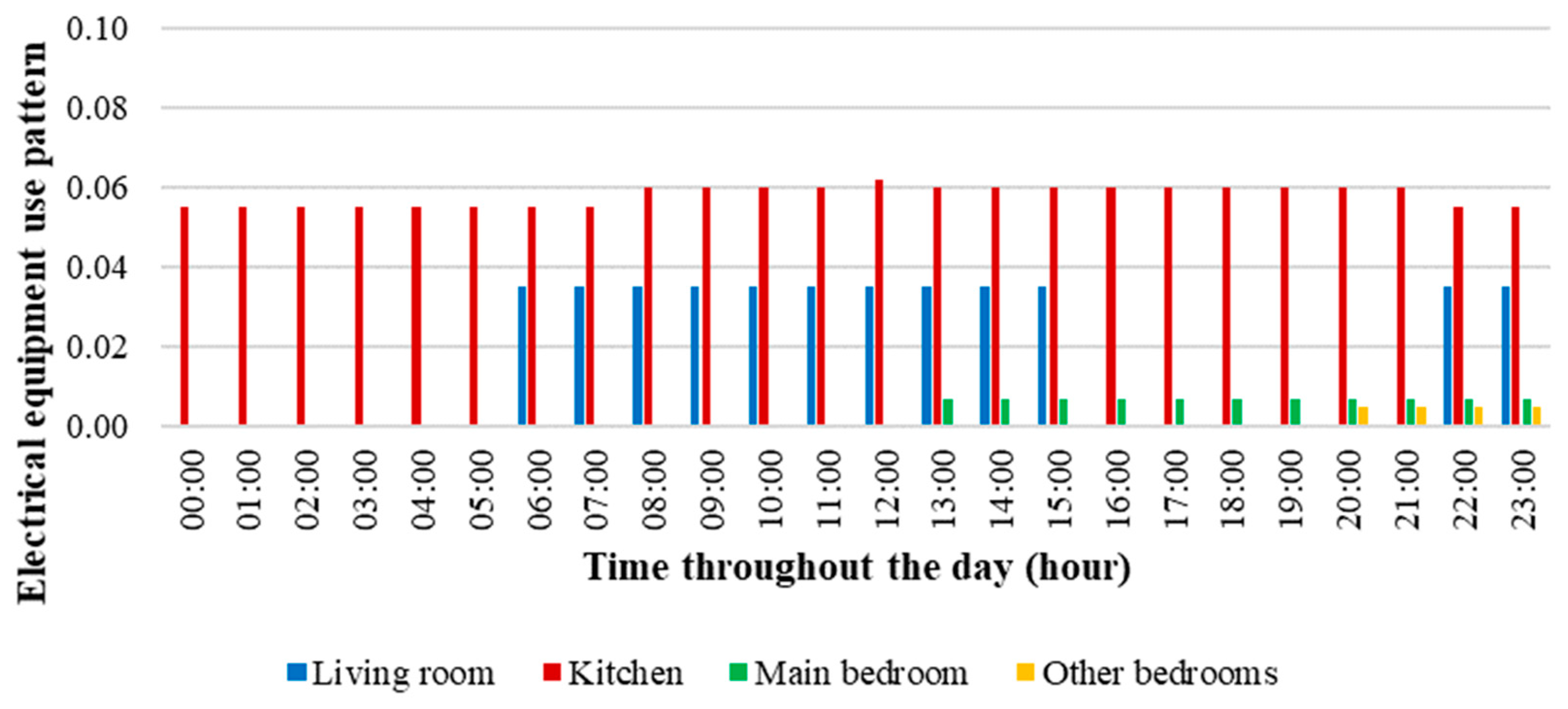
| Use and Operation Patterns | ||||
|---|---|---|---|---|
| Artificial Lighting | Environment | |||
| Lightning turned on | Living room | Kitchen | Main bedroom | Other bedrooms |
| 18:00–23:59 | 18:00–23:59 | 21:00–23:59 | 20:00–21:59 | |
| Openings operation | Openings | |||
| Openings opened | External door | Internal doors | Living room and kitchen windows | Bedrooms windows |
| 08:00–19:59 | 08:00–22:59 | 08:00–22:59 | 08:00–17:59 | |
| Step | Stop Rule | ||
|---|---|---|---|
| Number of Clusters in Each Step | Agglomeration Coefficient | Increase in the Agglomeration Coefficient Compared to the Previous Step (%) | |
| (Previous steps omitted) | |||
| 98 | 8 | 424.6 | 8.6 |
| 99 | 7 | 466.9 | 9.9 |
| 100 | 6 | 517.0 | 10.7 |
| 101 | 5 | 587.9 | 13.7 |
| 102 | 4 | 679.3 | 15.5 |
| 103 | 3 | 772.9 | 13.7 |
| 104 | 2 | 929.2 | 20.2 |
| 105 | 1 | 1155.0 | 24.2 |
| Variables | Two-Cluster Solution | Three-Cluster Solution |
|---|---|---|
| (p-Value < 0.05) | (p-Value < 0.05) | |
| Dry areas wall composition | <0.00 | <0.00 |
| Wet areas wall composition | 0.25 | 0.48 |
| Dry areas floor composition | <0.00 | <0.00 |
| Wet areas floor composition | <0.00 | <0.00 |
| Ground contact | <0.00 | <0.00 |
| Tile type | 0.25 | 0.00 |
| Existence of concrete slab on the roof | 0.04 | <0.00 |
| Ceiling material | 0.48 | <0.00 |
| Door frame material | 0.30 | 0.22 |
| Windows frame material | 0.02 | 0.07 |
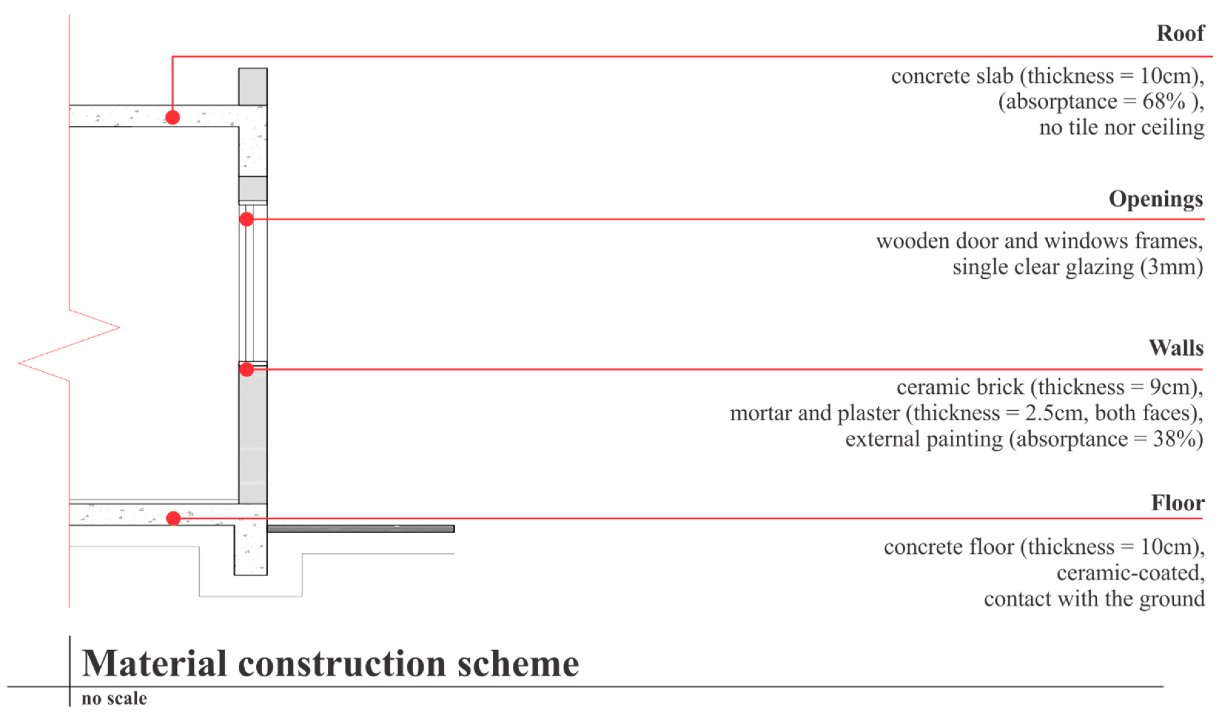
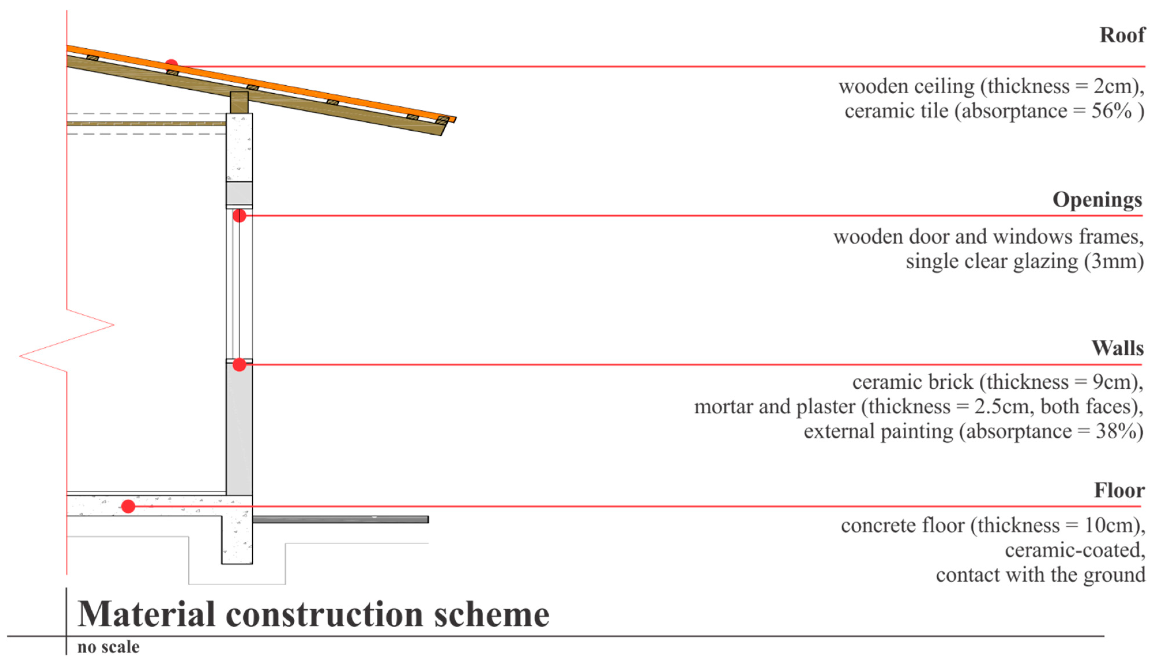
| Variables | Two Clusters Solution | Three Clusters Solution | |||
|---|---|---|---|---|---|
| Cluster 1 | Cluster 2 | Cluster 1 | Cluster 2 | Cluster 3 | |
| Dry areas wall composition | Ceramic brick | Wood | Ceramic brick | Ceramic brick | Wood |
| Wet areas wall composition | Ceramic brick | Ceramic brick | Ceramic brick | Ceramic brick | Ceramic brick |
| Dry areas floor composition | Ceramic-coated concrete floor | Wood | Ceramic-coated concrete floor | Ceramic-coated concrete floor | Wood |
| Wet areas floor composition | Ceramic-coated concrete floor | Ceramic-coated concrete floor | Ceramic-coated concrete floor | Ceramic-coated concrete floor | Ceramic-coated concrete floor |
| Ground contact | Yes | No | Yes | Yes | No |
| Tile type | Ceramic tile | Fibre cement tile | None | Ceramic tile | Fibre cement tile |
| Existence of concrete slab on the roof | No | No | Yes | No | No |
| Ceiling material | Wood | Wood | None | Wood | Wood |
| Door frame material | Wood | Wood | Wood | Wood | Wood |
| Windows frame material | Wood | Wood | Wood | Wood | Wood |
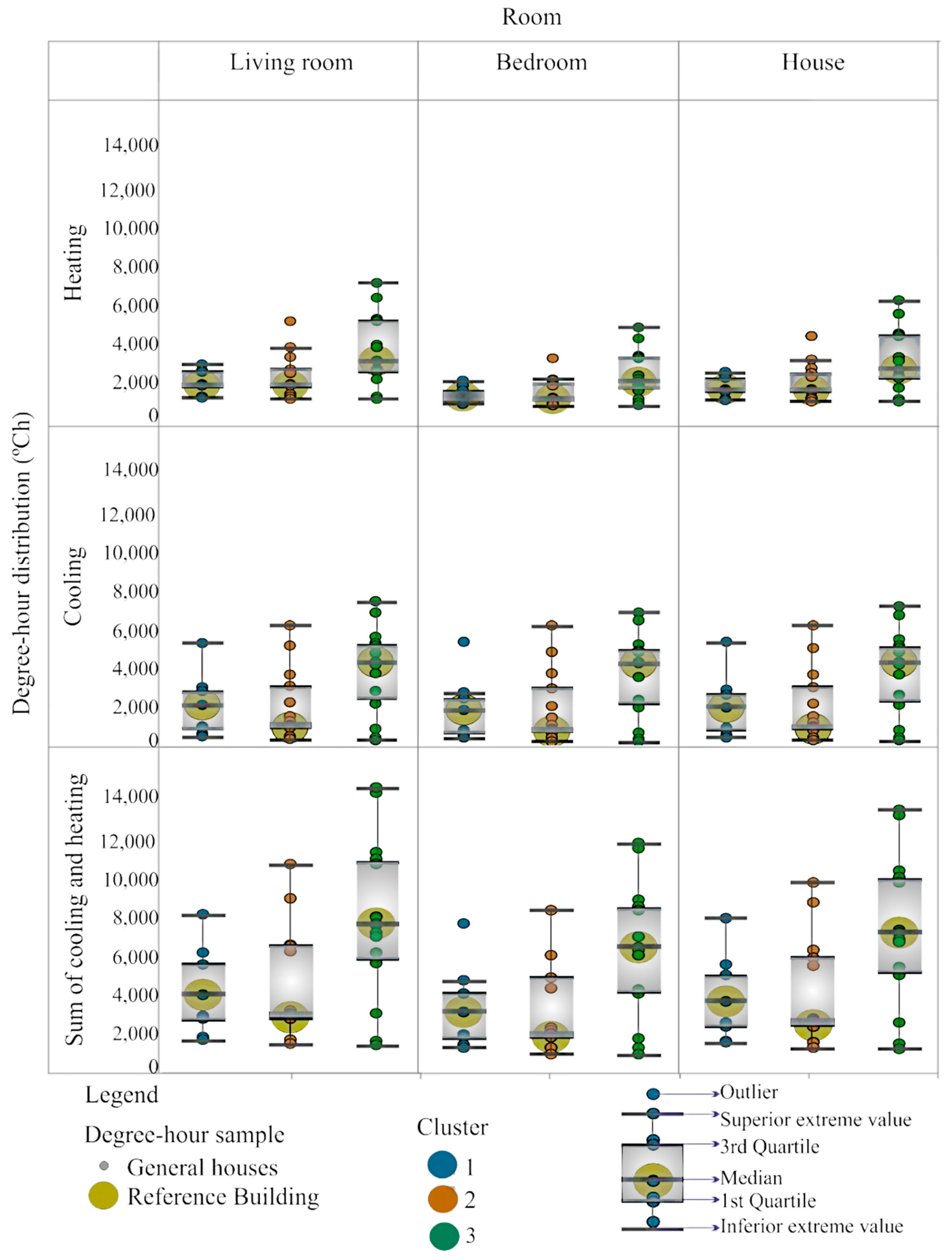
| Rooms | Annual Degree-Hour | Cluster 1 (26 Houses) | Cluster 2 (50 Houses) | Cluster 3 (30 Houses) | p-Value | |||
|---|---|---|---|---|---|---|---|---|
| Mean (°Ch) | Sd. Error (°Ch) | Mean (°Ch) | Sd. Error (°Ch) | Mean (°Ch) | Sd. Error (°Ch) | |||
| Living room | Cooling | 1358 | 231 | 1081 | 143 | 3861 | 380 | <0.00 |
| Heating | 1553 | 99 | 1713 | 91 | 3473 | 325 | <0.00 | |
| Total | 2925 | 332 | 2807 | 235 | 7334 | 708 | <0.00 | |
| Bedroom | Cooling | 1206 | 225 | 910 | 144 | 3688 | 364 | <0.00 |
| Heating | 1066 | 61 | 1047 | 56 | 2242 | 209 | <0.00 | |
| Total | 2283 | 288 | 1967 | 201 | 5929 | 577 | <0.00 | |
| House | Cooling | 1299 | 228 | 1014 | 143 | 3793 | 374 | <0.00 |
| Heating | 1361 | 83 | 1451 | 77 | 2988 | 279 | <0.00 | |
| Total | 2660 | 305 | 2464 | 210 | 6781 | 627 | <0.00 | |
Disclaimer/Publisher’s Note: The statements, opinions and data contained in all publications are solely those of the individual author(s) and contributor(s) and not of MDPI and/or the editor(s). MDPI and/or the editor(s) disclaim responsibility for any injury to people or property resulting from any ideas, methods, instructions or products referred to in the content. |
© 2023 by the authors. Licensee MDPI, Basel, Switzerland. This article is an open access article distributed under the terms and conditions of the Creative Commons Attribution (CC BY) license (https://creativecommons.org/licenses/by/4.0/).
Share and Cite
Schaefer, A.; Scolaro, T.P.; Ghisi, E. Finding Patterns of Construction Systems in Low-Income Housing for Thermal and Energy Performance Evaluation through Cluster Analysis. Sustainability 2023, 15, 12793. https://doi.org/10.3390/su151712793
Schaefer A, Scolaro TP, Ghisi E. Finding Patterns of Construction Systems in Low-Income Housing for Thermal and Energy Performance Evaluation through Cluster Analysis. Sustainability. 2023; 15(17):12793. https://doi.org/10.3390/su151712793
Chicago/Turabian StyleSchaefer, Aline, Taylana Piccinini Scolaro, and Enedir Ghisi. 2023. "Finding Patterns of Construction Systems in Low-Income Housing for Thermal and Energy Performance Evaluation through Cluster Analysis" Sustainability 15, no. 17: 12793. https://doi.org/10.3390/su151712793